Collision-Free 4D Dynamic Path Planning for Multiple UAVs Based on Dynamic Priority RRT* and Artificial Potential Field

Abstract

In this paper, a four-dimensional (4D) dynamic cooperative path planning algorithm for multiple unmanned aerial vehicles (UAVs) is proposed, in which the cooperative time variables of UAVs, as well as conflict and threat avoidance, are considered. The algorithm proposed in this paper uses a hierarchical framework that is divided into a 4D cooperative planning layer and a local threat avoidance planning layer. In the cooperative planning layer, the proposed algorithm, named dynamic priority rapidly exploring random trees (DPRRT*), would be used for the 4D cooperative path planning of all UAVs involved in a given task. We first designed a heuristic prioritization strategy in the DPRRT* algorithm to rank all UAVs to improve the efficiency of cooperative planning. Then, the improved RRT* algorithm with the 4D coordination cost function was used to plan the 4D coordination path for each UAV. Whenever the environment changes dynamically (i.e., sudden static or moving threats), the proposed heuristic artificial potential field algorithm (HAPF) in the local threat avoidance planning layer is used to plan the local collision avoidance path. After completing local obstacle avoidance planning, the DPRRT* of the 4D cooperative planning layer is again called upon for path replanning to finally realize 4D cooperative path planning for all UAVs. The simulation and comparison experiments prove the feasibility, efficiency, and robustness of the proposed algorithm.

1. Introduction

In recent years, UAVs have been widely used in both military and civilian fields, such as urban penetration, battlefield reconnaissance, aerial photography, disaster area search and rescue, etc. [1,2]. However, with the increasing diversification of missions and the complexity of flight environments, more and more users are reaching the limitations of single UAVs when performing missions [3]. Therefore, multiple UAV systems have gradually grown into a popular and challenging research topic [4]. As the most basic problem in the research of multi-UAV systems, the cooperative path planning technology of multiple UAVs directly affects the ability of UAVs to complete tasks smoothly, safely, and autonomously [5,6].

Multi-UAV systems are usually deployed for more complex tasks, such as coordinated multi-UAV attack and detection missions, which require all UAVs to have the same and shortest arrival time [7]. In addition, since there are usually a variety of threats in flight environments where multiple UAV systems perform tasks, the planning of a safe path that must simultaneously avoid environmental threats and collisions between individual UAVs is a difficult problem [8]. Furthermore, ground-based navigation systems are often unable to detect the precise location and configuration information of all threats in complex environments [9]. Therefore, it is particularly difficult to coordinate the paths of all UAVs involved and adjust their existing paths in a timely and efficient manner according to real-time environmental information [10], especially for some tasks that require accurate arrival time and dynamic conflict avoidance simultaneously.

The existing methods of solving the cooperative path planning problem of multiple UAVs include several collision avoidance methods and cooperative path generation methods [11]. Collision avoidance methods are often used to deal with local spatial conflicts. First, each UAV independently plans the shortest path while avoiding threats in the environment. During the path execution, each UAV regularly detects the position and speed of other UAVs around it. If there is a risk of collision, the UAVs adjust their paths in real time to avoid conflicts. Many local collision avoidance path planning algorithms based on collision avoidance methods have been proposed, such as the artificial potential field algorithm (APF) [12,13], the centralized control barrier function algorithm (CCBF) [14], the distributed control barrier function algorithm (DCBF) [15], and the optimal reciprocal collision avoidance algorithm (ORCA) [16]. Since collision avoidance is only performed in a local range, these algorithms usually have high computational efficiency and the ability to dynamically and rapidly replan paths. However, as a local collision avoidance method, with the increase in the number of UAVs and threats, these algorithms may fall into local minima and lead to the failure of cooperative path planning. Additionally, since such methods focus on space conflict avoidance, the consistency of flight time is not considered.

Cooperative path generation methods can be divided into two categories: coupling methods and decoupling methods [17]. The coupling method usually regards all UAVs as comprising an agent system and directly searches for the cooperative path of the agent system. Some popular coupling methods, such as increasing cost tree search (ICTS) [18] and conflict-based search (CBS) [19], have been extensively studied and many variant algorithms have been derived [20,21,22,23]. The coupling method directly deals with the path planning problem of the agent system and can usually obtain the optimal solution for the system. However, it is well-known that even a simple variant of the path planning problem for multiple UAVs, such as a planned cooperative path with the sudden appearance of a threat, interferes with the implementation of a cooperative path that encounters both conflict-free space and path execution time consistency. In addition, in computing, the coupling method is very difficult to solve [24].

Decoupling methods usually divide the problem of multi-UAV cooperative path planning into two steps, i.e., the coordination of the path planning sequence and the single UAV cooperative path planning [25]. As the most representative algorithm of the decoupling method, the prioritized planning algorithm (PP) [26] has become a very popular algorithm in cooperative path planning [27], along with other methods such as the revised prioritized planning algorithm (RPP) [28], the decentralized prioritized planning (DPP) [29], and the asynchronous decentralized prioritized planning algorithm (ADPP) [30]. In the prioritized planning algorithm, each UAV has its own priority and calculates its path according to the relative order of its priority. Therefore, the final path of each UAV is able to avoid static threats in the environment and UAVs with a higher priority than it. The common single UAV cooperative path planning algorithms in prioritized planning algorithms are the grid-based A* algorithm [31] and the sample-based RRT* algorithm [32,33]. The calculation time of the A* algorithm usually increases exponentially with the increase in spatial dimension and grid resolution, and it does not perform well in large planning spaces of UAVs [34]. The RRT* algorithm is able to reach the optimal solution with fewer samples than the fixed high-resolution grid method by sampling the extended tree structure. Therefore, RRT* is widely used in path planning in high-dimensional space [35]. Furthermore, if the priority can be assigned reasonably, the prioritized planning algorithm can usually plan the cooperative path for multiple UAVs more efficiently. The existing decoupling methods also focus on conflict avoidance and do not conduct in-depth research on the time consistency of all UAV planning paths. In addition, in complex environments with unknown threats, the ability of the existing decoupling methods to avoid dynamic sudden threats is unknown.

Therefore, combining the practical applications of the environment and the complex task categories of multiple UAV systems, as well as the possible improvement of existing path planning algorithms for multiple UAVs, the main motivations of this paper are as follows.

• The actual flight environment of UAVs is mostly wide open space. Due to the complexity of the actual flight environment, certain detected static threats can suddenly start to move and previously unknown static or moving threats can suddenly appear. Only relying on the known environment broadcast by the navigation system for cooperative path planning often carries the risk of unfeasible paths being followed.
• The tasks performed by multi-UAV systems have gradually become more complex and diverse. Three-dimensional cooperative planning based on conflict-free space no longer meets the needs of most tasks.
• Existing algorithms based on the local collision avoidance method, the coupling method, and the decoupling method are rarely studied in the field of 4D cooperative path planning [36,37]. In addition, the local collision avoidance method is able to adapt to the frequently changing dynamic environment but cannot ensure the success of global cooperative path planning. The decoupling method can quickly plan cooperative paths for multiple UAVs but it cannot guarantee the efficiency of cooperative replanning brought about by environmental changes.

Therefore, this paper focuses on the research of a 4D dynamic cooperative path planning algorithm for multiple UAVs. The algorithm needs to be consistent in terms of the conflict-free space and flight time of multiple UAVs simultaneously and must be able to adapt to frequent changes in the environment so that the algorithm can quickly avoid threats and suddenly encountered threats and ensure a lack of conflict between UAVs. More specifically, the algorithm proposed in this paper adopts a hierarchical strategy for the 4D cooperative path planning of multiple UAVs and the local cooperative collision avoidance planning for dynamic environments. The 4D cooperative planning algorithm based on DPRRT* consists of a heuristic dynamic prioritization strategy, priority planning order coordination, and an improved RRT* algorithm based on 4D cooperative constraints. The local threat avoidance planner based on HAPF effectively overcomes the problems of unreachable targets, the risks of falling into local minima, and the path oscillation which exists in traditional APF by improving potential field functions, heuristic optimal sub-target node selection strategies and memory resultant force strategies, respectively. In fact, the proposed algorithm based on a hierarchical strategy combines the advantages of the decoupling method and the collision avoidance method and overcomes their shortcomings. In addition, the algorithms based on the two methods are improved and upgraded to be used for more extensive practical applications in the future.

Overall, the main contributions of this paper are as follows:

• A 4D dynamic cooperative path planning algorithm based on a hierarchical strategy is proposed. The proposed upper layer based on DPRRT* is able to plan a 4D cooperative path for UAVs that simultaneously meets the requirements of conflict-free space and consistent flight time. The proposed lower layer based on HAPF is able to deal with online dynamic local collision avoidance planning in frequently changing environments.
• In the proposed DPRRT* algorithm, a heuristic dynamic prioritization strategy was designed. Within a planned environment, the heuristic prioritization algorithm was used to reasonably and dynamically adjust the priorities of UAVs to efficiently and robustly plan their path generation sequences.
• In the single-UAV planning algorithm of DPRRT*, a 4D cost function based on time cooperative constraints was proposed, which guides the expansion of new nodes and the optimization process of neighborhood nodes to quickly plan a path that satisfies the 4D cooperative constraints of UAVs.
• In HAPF, a heuristic sub-target node selection strategy was designed to select the optimal sub-target node for the UAVs in local obstacle avoidance planning in order to get rid of the local minimum node. In addition, a memory resultant force strategy was designed to improve path oscillation, so that the obstacle avoidance path is smoother and is able to meet the performance constraints of the UAVs.

This paper is organized as follows. Section 2 describes the 4D dynamic cooperative path planning problem. In Section 3, the 4D dynamic cooperative path planning algorithm proposed in this paper is explained in detail. Section 4 outlines the simulation and comparison experiments of the proposed algorithm and discusses the simulation results. Section 5 describes some of the conclusions reached, as well as future works.

2. Problem Formulation

The 4D multi-UAV dynamic cooperative path planning problem discussed in this paper refers to a problem in dynamic 4D space $\mathcal{X}\left(x,y,z,t\right)\subseteq {\mathbb{R}}^4$ comprising sudden threats for each UAV in the group, ${\mathrm{UAV}}_N:\left({\mathrm{UAV}}_1,\dots ,{\mathrm{UAV}}_n\right)$, composed of $n$ UAVs, resulting in the planning of a path that meets 4D cooperative constraints and involves no collisions with threats in the dynamic environment.

Considering the diversity of tasks performed by UAV groups, the starting node or end node of multiple UAVs may overlap (such as in rendezvous tasks), so this paper assumes that if multiple UAVs have the same start node or goal, there will be no collision. In addition, each UAV has communication equipment to relay information. This paper assumes that communication is completely reliable and there are no delays.

2.1. Dynamic Cooperative Path Planning Constraints of UAVs

For the constraints of the general UAV’s 4D dynamic cooperative path planning, the UAV performance constraints, dynamic environment limitations, and 4D cooperative constraints should be considered. Each ${\mathrm{UAV}}_i$ in ${\mathrm{UAV}}_N$ needs to take off from its own starting node at the same time. The planned path needs to avoid conflicts with the other ${\mathrm{UAV}}_{N/i}:{\mathrm{UAV}}_N\backslash {\mathrm{UAV}}_i$ while avoiding all threats (including radar, anti-aircraft artillery, anti-aircraft missiles, and terrain) and finally reaching the intended goal at the same time. The planned path needs to take into consideration the performance constraints of the UAV. In addition, sudden, undetected threats may appear during flight, i.e., the planning space is dynamic. Therefore, the UAVs affected by the change of environment need to carry out local path replanning to avoid these threats. Note that the local path replanning destroys the 4D cooperative constraints, making it also necessary to carry out cooperative replanning for each ${\mathrm{UAV}}_N$ to allow the path to meet the cooperative path planning requirements of the UAV.

2.1.1. UAV Performance Constraints

The cooperative path, ${\sigma }_i$, of any ${\mathrm{UAV}}_i$ in ${\mathrm{UAV}}_N$ is composed of a group of path nodes $P_i:\left\{\left(p_1,\dots ,p_K\right)\left|p_1=s_i,p_K=g_i,p_k=\left(x_k,y_k,z_k,t_k\right)\right.\right\}$. ${\sigma }_i$ needs to meet the performance constraints of the UAVs, including the maximum flight distance $L_{\max }$, the maximum steering angle ${\varphi }_{\max }$, the maximum climbing/diving angle ${\gamma }_{\max }$, and the shortest path segment distance $l_{\min }$. UAV performance constraints are shown in Definition 1.

Definition 1 (UAV performance constraints).

For any ${\mathrm{UAV}}_i$ in-planning space $\mathcal{X}$, the maximum flight distance constraint is:

$$L_{{\mathrm{UAV}}_i}={\displaystyle \sum _{i=0}^k\sqrt{{(x_{i+1}-x_i)}^2+{(y_{i+1}-y_i)}^2+{(z_{i+1}-z_i)}^2}}\le L_{\max }$$

(1)

and the maximum steering angle constraint is:

$$\left|{\varphi }_{{\mathrm{UAV}}_i}\right|=\left|\frac{{\lambda }_i^T{\lambda }_{i+1}}{{‖{\lambda }_i‖}_2·{‖{\lambda }_{i+1}‖}_2}\right|\le {\varphi }_{\max }$$

(2)

where ${\lambda }_i={[x_i-x_{i-1},y_i-y_{i-1}]}^T$.

The maximum climbing/diving angle constraint is:

$$\left|{\gamma }_{{\mathrm{UAV}}_i}\right|=\left|\arcsin (\frac{z_i-z_{i-1}}{{‖{\lambda }_i‖}_2})\right|\le {\gamma }_{\max }$$

(3)

and the shortest path segment distance constraint is:

$$l_{{}_{{\mathrm{UAV}}_i}}={‖p_{i+1}-p_i‖}_2\ge l_{\min }$$

(4)

2.1.2. Environmental Limitations

In the dynamic planning environment, there are five different types of threats, i.e., terrain threats, radar, anti-aircraft artillery, missiles, and sudden threats. Of these, the sudden threats refer to threats that suddenly appear (i.e., radar, anti-aircraft artillery, and missiles). Sudden threats can be static or moving. The modeling process of the first four threats has been described in detail in our previous work [38]. This paper mainly describes sudden threats and environmental limitations.

Considering the time uncertainty and state uncertainty of sudden threats, we describe the sudden threats in Definition 2.

Definition 2 (sudden threats).

For planning space $\mathcal{X}$, all UAVs in ${\mathrm{UAV}}_N$ fly according to the currently planned cooperative path, and the flight time interval is $\left[t_s,t_g\right]$. At $t\in \left[t_s,t_g\right]$, $m$ new threats ${\mathcal{X}}_{new}^{threat}:\left\{{\mathcal{X}}_1^{threat},\dots ,{\mathcal{X}}_m^{threat}\right\}$ are sudden threats. The position change rule ${\mathcal{X}}_{new}^{threat}$ is expressed as:

$$\Delta {\mathcal{X}}_{new}^{threat}={\displaystyle \underset{i=1}{\overset{m}{\cup }}\Delta {\mathcal{X}}_m^{threat}}, \mathrm{where} \Delta {\mathcal{X}}_m^{threat}=\left\{\begin{array}{l}\varnothing \\ f\left(x,t_i\right)\\ \mathrm{unpredictable}\end{array}\right.$$

(5)

where $\Delta {\mathcal{X}}_m^{threat}=\varnothing$ means that the sudden threat is static, $\Delta {\mathcal{X}}_m^{threat}=f\left(x,t_i\right)$ means that the dynamic sudden threat is moving, and $\Delta {\mathcal{X}}_m^{threat}=\mathrm{unpredictable}$ means that the threat movement is unpredictable.

The definition of environmental limitations is given in Definition 3.

Definition 3 (environmental limitations).

For any ${\mathrm{UAV}}_i$ in-planning space $\mathcal{X}$, the limit of the planning environment is:

$$\left\{\begin{array}{l}{z}_i-z_{{\left(x_i,y_i\right)}_{DMG}}\ge h_{\min }\\ \left(p_i,p_{i+1}\right)\cap {\mathcal{X}}^{threat}=\varnothing \end{array}\right.$$

(6)

where $z_{{\left(x_i,y_i\right)}_{DMG}}$ represents the terrain threat altitude when the UAV is located at $p_i$ and ${\mathcal{X}}^{threat}=\left\{{\mathcal{X}}_{known}^{threat}\cup {\mathcal{X}}_{new}^{threat}\right\}$ represents the known radar, anti-aircraft artillery, and missile threats, as well as sudden threats.

2.1.3. Four-Dimensional Coordination Constraints

The four-dimensional coordination constraints consist of spatial coordination constraints and time coordination constraints. In this paper, it is assumed that any ${\mathrm{UAV}}_i$ in ${\mathrm{UAV}}_N$ flies at a uniform speed in any speed interval $\left[{\mathcal{V}}_{\min },{\mathcal{V}}_{\max }\right]$; that is, the estimated time of arrival (ETA) interval of ${\mathrm{UAV}}_i$ is $\left[t_{\min }^i={\sigma }_i/{\mathcal{V}}_{\max },t_{\max }^i={\sigma }_i/{\mathcal{V}}_{\max }\right]$.

Definition 4 (four-dimensional coordination constraints).

The cooperative path of all UAVs in ${\mathrm{UAV}}_N$ must meet the following requirements:

1. 

At moment $t$, the distance $D_{i,j}\left(t\right)$ between any two UAVs is:

$$D_{i,j}\left(t\right)={‖{\sigma }_i\left(t\right)-{\sigma }_j\left(t\right)‖}_2\ge D_{\min } \mathrm{i},\mathrm{j}=1,2,\dots ,k,i\ne j$$

(7)

where $D_{\min }$ is the minimum safe distance.

2. 

The set $T$ of ETA of all UAVs is:

$$T={\displaystyle \underset{i=1}{\overset{n}{\cap }}\left[t_{\min }^i,t_{\max }^i\right]}\ne \varnothing$$

(8)

2.2. Dynamic 4D Cooperative Path Planning Formulation

A set of 4D cooperative paths for ${\mathrm{UAV}}_N$ can be obtained only when Definitions 1, 3, and 4 are met.

Problem 1 describes the 4D dynamic cooperative path planning problem of the multiple UAVs studied in this paper.

Problem 1 (dynamic 4D cooperative path planning).

In the current dynamic planning space $\mathcal{X}$, the set starting nodes and goal nodes $\left[s_1,g_1\right],\dots ,\left[s_n,g_n\right]$ of all UAVs in ${\mathrm{UAV}}_N$ are given. A group of paths ${\sigma }_N=\left\{{\sigma }_1,\dots ,{\sigma }_n\right\}$ must be found so that all paths in ${\sigma }_N$ meet the necessary constraints of Definitions 1, 3, and 4.

3. Four-Dimensional Dynamic Cooperative Path Planning Algorithm

The overall frameworks of the 4D dynamic cooperative path planning algorithm, the DPRRT* algorithm, and the HAPF algorithm will be introduced below.

3.1. Overall Framework

Algorithm 1 shows the executive process of the 4D dynamic cooperative path planning algorithm for multiple UAVs.

Algorithm 1. Four dimensional Dynamic Cooperative Path Planning Algorithm for Multiple UAVs

$\begin{array}{l}01: \mathsf{MAIN} \mathsf{ALGORITHM}\\ 02: initialization \mathcal{X},{\mathcal{T}}_i\leftarrow \varnothing , {\sigma }_i\left(t\right)\leftarrow \varnothing , \left[s_1,g_1\right],\dots ,\left[s_n,g_n\right],\mathit{\sigma }\left(t\right)\leftarrow \left[{\sigma }_1\left(t\right),\dots ,{\sigma }_n\left(t\right)\right],\\ Len\_cost\left(t\right)\leftarrow \left[{Len\_cost}_1\left(t\right),\dots {,Len\_cost}_n\left(t\right)\right]\\ 03: \left({Len\_cost}_i,{\sigma }_i\left(t\right)\right)\leftarrow \mathit{R}\mathit{R}\mathit{T}*\left(\mathcal{X},{\mathcal{T}}_i,s_i,g_i\right) /*\mathit{Synchronous} \mathit{execution} \mathit{of} \mathit{all} \mathit{UAVs}*/\\ 04: \mathbf{wait} \mathrm{for} \mathrm{all} \mathrm{UAVs} \mathrm{to} \mathrm{finish} \mathrm{planning} \mathrm{their} \mathrm{own} {\sigma }_i \mathrm{and} {\mathit{Len}\_\mathit{cos}t}_i\\ 05: \left[t_{co},l_{co}\right]\leftarrow \mathit{E}\mathit{T}\mathit{A}\_\mathit{L}\mathit{e}\mathit{n}\left(\mathit{\sigma }\left(t\right),Len\_cost\left(t\right)\right)\\ 06: \mathit{\sigma }\left(t\right)\leftarrow \mathit{D}\mathit{P}\mathit{R}\mathit{R}\mathit{T}*\left(\mathcal{X},t_{co},l_{co},\left[s_1,g_1\right],\dots ,\left[s_n,g_n\right],\mathit{\sigma }\right)\\ 07: \mathrm{all} \mathrm{UAVs} \mathrm{move} \mathrm{along} \mathit{\sigma }\left(t\right)\\ 08: while \mathrm{goal} \mathrm{not} \mathrm{reach} and \Delta {\mathcal{X}}_{new}^{threat} \mathrm{detected}\\ 09: \mathcal{X}\leftarrow \mathcal{X}\cup \Delta {\mathcal{X}}_{new}^{threat}\\ 10: \left({\mathit{\sigma }}_{conflict},UA{V}_{conflict}\right)\leftarrow \mathit{C}\mathit{o}\mathit{n}\mathit{f}\mathit{l}\mathit{i}\mathit{c}\mathit{t}\mathit{s}\_\mathit{o}\mathit{c}\mathit{c}\mathit{u}\mathit{r}\mathit{r}\mathit{e}\mathit{d}\left(\mathit{\sigma },\Delta {\mathcal{X}}_{new}^{threat}\right)\\ 11: if {\mathit{\sigma }}_{conflict}\ne \varnothing \\ 12:{ \mathrm{t}}_0\leftarrow clock\left(\right)\\ 13: \mathit{H}\mathit{A}\mathit{P}\mathit{F}\left(UA{V}_{conflict},\mathcal{X}\cup \left(\mathit{\sigma }\left(t_0,t_{co}\right)\backslash {\mathit{\sigma }}_{conflict}\left(t_0,t_{co}\right)\right)\right)\\ /*\mathit{Synchronous} \mathit{execution} \mathit{of} UA{V}_{conflict}*/\\ 14: \mathrm{all} UAV\backslash UA{V}_{conflict} \mathrm{and} \mathrm{UAVs} \mathrm{which} \mathrm{finish} \mathit{H}\mathit{A}\mathit{P}\mathit{F} \mathrm{move} \mathrm{along} theirown{\mathsf{\sigma }}_{\mathrm{i}}\\ /*\mathit{Synchronous} \mathit{execution} \mathit{with} 13*/\\ 15: else \\ 16: \mathrm{all} \mathrm{UAVs} \mathrm{move} \mathrm{along} \mathit{\sigma }\left(t_0,t_{co}\right)\\ 17: end if\\ 18:{ \mathrm{t}}_0\leftarrow clock\left(\right)\\ 19: \left[t_{co},l_{co}\right]\leftarrow \mathit{E}\mathit{T}\mathit{A}\_\mathit{L}\mathit{e}\mathit{n}\left(\mathit{\sigma }\left(t_0,t_{co}\right),Len\_cost\left(t_0,t_{co}\right)\right)\\ 20: \mathit{\sigma }\left(t_0,t_{co}\right)\leftarrow \mathit{D}\mathit{P}\mathit{R}\mathit{R}\mathit{T}*\left(\mathcal{X},t_{co},\left[{\sigma }_1\left(t_0\right),g_1\right],\dots ,\left[{\sigma }_n\left(t_0\right),g_n\right],\mathit{\sigma }\right)\\ 21: \mathrm{all} \mathrm{UAVs} \mathrm{move} \mathrm{along} \mathit{\sigma }\left(t_0,t_{co}\right)\\ 22: end while\end{array}$

In the pre-cooperative planning based on the initial environment (lines 02–07), the algorithm first initializes the search tree $T_i$ and sets the start and goal $\left[s_i,g_i\right]$ of any ${\mathrm{UAV}}_i$, as well as the initial planning space $\mathcal{X}$. Then, the classical RRT* shown in Algorithm 1 is used to plan the optimal path for all UAVs without considering the 4D cooperative constraints. After the UAV planning is completed, the shortest coordination time $t_{co}$ of the UAVs is determined through the process $\mathit{E}\mathit{T}\mathit{A}\_\mathit{L}\mathit{e}\mathit{n}$. Then, the DPRRT* algorithm is used to plan the paths of all UAVs that meet the 4D cooperative constraints in the initial planning space $\mathcal{X}$. Finally, all UAVs execute their respective cooperative paths.

The purpose of the process $\mathit{E}\mathit{T}\mathit{A}\_\mathit{L}\mathit{e}\mathit{n}$ is to obtain the minimum coordination time $t_{co}$ of all the UAVs by calculating the minimum flight time set for all UAVs and calculating the maximum value in the set. It should be noted that all UAVs can achieve the shortest path (Line 03) through classical RRT*. In other words, all UAVs are able to achieve the shortest flight time without considering 4D cooperative constraints. We assume that the minimum flight time ${\mathrm{UAV}}_i$ is $t_i$, the minimum flight time ${\mathrm{UAV}}_j$ is $t_j$, and that $t_i>t_j$. Since $t_i$ and $t_j$ are already the shortest flight times, the only way to ensure that ${\mathrm{UAV}}_i$ and ${\mathrm{UAV}}_j$ satisfy the time coordination constraints and ensure the shortest coordination time is to increase $t_i$ so that it is equal to $t_j$.

If the UAV detects a sudden threat $\Delta {\mathcal{X}}_{new}^{threat}$ in planning space $\mathcal{X}$ during flight, the cooperative path based on the previous planning space may be affected, resulting in the failure of the path to cooperate. Therefore, cooperative replanning needs to be executed in the new planning space containing $\Delta {\mathcal{X}}_{new}^{threat}$. We use the $\mathit{C}\mathit{o}\mathit{n}\mathit{f}\mathit{l}\mathit{i}\mathit{c}\mathit{t}\mathit{s}\_\mathit{o}\mathit{c}\mathit{c}\mathit{u}\mathit{r}\mathit{r}\mathit{e}\mathit{d}$ process to find the UAV set $UA{V}_{conflict}$ (and its conflict path ${\mathit{\sigma }}_{conflict}$) affected by $\Delta {\mathcal{X}}_{new}^{threat}$ from among all UAVs. Then, HAPF is applied to all UAVs in the set $UA{V}_{conflict}$ for the efficient online onboard replanning of paths. As HAPF is a local conflict avoidance algorithm, it can only ensure that the UAV meets the spatial coordination constraints in the 4D coordination constraints. Therefore, we choose the path node ${\mathit{\sigma }}_{conflict}$ which, as the generation node of the attractive potential field of $UA{V}_{conflict}$, is not reached and not affected by the threat, thus enabling $UA{V}_{conflict}$ to return to the previous 4D cooperative path after avoiding the sudden threat. At the same time, the UAVs not affected by $\Delta {\mathcal{X}}_{new}^{threat}$ continue to fly along the previously planned coordinated path. When the $UA{V}_{conflict}$ avoids sudden threats, the DPRRT* is used to replan the path from the current position of the UAVs to their destination, while meeting the 4D cooperative constraints for all UAVs. If the planning space is not changed, all UAVs fly along the current initial path until they reach the goal and the algorithm is terminated. Otherwise, when new sudden threats are detected, lines 08–22 of Algorithm 1 are executed until the goal is reached.

3.2. Dynamic Priority RRT* Algorithm

In the cooperative path planning layer, we used the proposed DPRRT* to complete the 4D cooperative path planning of multiple UAVs based on the current initial planning space. The pseudo-code for DPRRT* is shown in Algorithm 2. The core idea of DPRRT* is to enable UAVs with lower priority to avoid conflict with the planned paths of the UAVs with higher priority when planning the cooperative paths in order to meet the requirements of 4D cooperative constraints.

Considering that the prioritization of UAVs usually has a great impact on the efficiency and robustness of cooperative path planning, we designed a dynamic heuristic prioritization strategy (i.e., the $\mathrm{HeuDyn}\_\mathrm{Proritization}$ process) to assign the priorities of all UAVs, where $\mathrm{UA}{\mathrm{V}}_i^j$ represents the priority of $\mathrm{UA}{\mathrm{V}}_i$ as $j$ and $\mathit{\sigma }\left(t\right)$ represents the planned cooperative path of the UAVs based on the previously planned space. Thereafter, the cooperative paths of all UAVs are planned in order of priority from high to low. In addition, in order to simultaneously meet the time and space cooperative constraints, this paper improves the classical RRT* to an RRT* algorithm based on 4D cooperative constraints, named 4DRRT* (i.e., the $4\mathrm{D}\mathrm{R}\mathrm{R}\mathrm{T}*$ process), so that each UAV is able to quickly plan a path that meets the cooperative 4D constraints. Note that before planning the lower-priority UAV paths, the planned paths of the high-priority UAVs need to be added to the space–time occupied area $H^j$ to ensure that the planned paths of the low-priority UAVs do not conflict with those of high-priority UAVs. The dynamic heuristic prioritization strategy and 4DRRT* algorithm will be introduced in detail below.

Algorithm 2. DPRRT* Algorithm

$\begin{array}{l}01: \mathsf{MAIN} \mathsf{ALGORITHM}\\ 02: H^j\leftarrow \varnothing , {\mathit{\sigma }}^{*}\leftarrow \varnothing \\ 03: {\displaystyle \underset{i,j=1}{\overset{N}{\cup }}\mathrm{UA}{\mathrm{V}}_i^j}\leftarrow \mathit{HeuDyn}\_\mathit{Proritization}\left(\mathit{\sigma }\left(t\right)\right)\\ 04: for j=1 \mathrm{to} N\\ 05: {\sigma }_i^j\left(t\right)\leftarrow \mathit{4}\mathit{D}\mathit{R}\mathit{R}\mathit{T}*\left(\mathcal{X},t_{co},H^j,s_i,g_i\right)\\ 06: H^j\leftarrow H^j\cup {\sigma }_i^j\left(t\right)\\ 07: {\mathit{\sigma }}^{*}\left(\mathrm{t}\right)\leftarrow {\sigma }_i^j\left(t\right)\cup {\mathit{\sigma }}^{*}\\ 08: end for\\ ----------------------------\\ 01: \mathsf{Function} \mathit{HeuDyn}\_\mathit{Proritization}\\ 02: f_{HDP}^{\mathrm{UA}{\mathrm{V}}_N}\leftarrow \varnothing ,k=1\\ 03: for i=1 \mathrm{to} N\\ 04: f_{HDP}^{{\mathrm{UAV}}_i^j}=\left|t_{co}-\frac{{\sigma }_i\left(t_0,t_{co}\right)}{v_i}\right|\\ 05: f_{HDP}^{\mathrm{UA}{\mathrm{V}}_N}\leftarrow f_{HDP}^{\mathrm{UA}{\mathrm{V}}_N}\cup \left\{f_{HDP}^{{\mathrm{UAV}}_i^j}\right\}\\ 06: end for\\ 07: while f_{HDP}^{\mathrm{UA}{\mathrm{V}}_N}\ne \varnothing \\ 08: \mathrm{UA}{\mathrm{V}}_i^k\leftarrow \arg \max f_{HDP}^{\mathrm{UA}{\mathrm{V}}_N}\\ 09: f_{HDP}^{\mathrm{UA}{\mathrm{V}}_N}\leftarrow f_{HDP}^{\mathrm{UA}{\mathrm{V}}_N}\backslash f_{HDP}^{\mathrm{UA}{\mathrm{V}}_i^k}\\ 10: k=k+1\\ 11: end while\\ ----------------------------\\ 01: \mathsf{Function} 4\mathit{D}\_\mathit{E}\mathit{x}\mathit{t}\mathit{a}\mathit{n}\mathit{d}\\ 02: for \mathrm{all} x_{\mathcal{T}}\in \mathcal{T}. V \mathrm{do}\\ 03: if \parallel x_{\mathcal{T}}-x_{rand}\parallel \le \delta \\ 04: { x}_{new}\leftarrow x_{rand}\\ 05: else\parallel x_{\mathcal{T}}-x_{rand}\parallel >\delta \\ 06: { x}_{new}\leftarrow x_{\mathcal{T}}+\delta \frac{x_{rand}-x_{\mathcal{T}}}{\parallel x_{rand}-x_v\parallel } \\ 07: end if\\ 08: if \mathit{obstacle}\_\mathit{f}\mathit{r}\mathit{e}\mathit{e}\left(x_{\mathcal{T}},x_{new}\right)\\ \wedge \mathit{UAV}\_\mathit{f}\mathit{r}\mathit{e}\mathit{e}\left(x_{\mathcal{T}},x_{new}\right)\\ \wedge \mathit{Conflict}\_\mathit{f}\mathit{r}\mathit{e}\mathit{e}\left(\left[x_{\mathcal{T}},x_{new}\right],H_i\right)\\ 09: f_{\mathcal{T}}^{4D}\left(x_{new}\right)\leftarrow \left|f_{\mathcal{T}}\left(x_{new}\right)-l_{co}\right|\\ 10: f_{\mathcal{T},all}^{4D}\leftarrow f_{\mathcal{T},all}^{4D}\cup f_{\mathcal{T}}^{4D}\left(x_{new}\right)\\ 11: end if\\ 12: end for\\ 13: x_{new}\leftarrow \mathrm{argmin} f_{\mathcal{T},all}^{4D}\end{array}$

$\begin{array}{l}01: \mathsf{Function} 4\mathit{D}\mathit{R}\mathit{R}\mathit{T}* (\mathrm{e}.\mathrm{g}., \mathrm{UA}{\mathrm{V}}_i)\\ 02: initialization \mathcal{T}.V\leftarrow \left\{s_i\right\};\mathcal{T}.E\leftarrow \varnothing \\ 03: L_{co}\leftarrow t_{co}{v}_i\\ 04: for i=1 \mathrm{to} n\\ 05: if P:\mathit{random}\left(\left[0,1\right]\right)<0.1\\ 06: x_{rand}\leftarrow g_i\\ 07: else\\ 08: x_{rand}\leftarrow \mathit{Sample}\left(\mathcal{X}\right)\\ 09: end if\\ 10: x_{new}\leftarrow 4\mathit{D}\_\mathit{E}\mathit{x}\mathit{t}\mathit{a}\mathit{n}\mathit{d}\left(x_{nearest}\right)\\ 11: \mathcal{T}.V\leftarrow \mathcal{T}.V\cup \left\{x_{new}\right\}\\ 12: end if\\ 13: X_{near}\leftarrow \mathit{Near}\left(x_{new},\mathcal{T}.V,\gamma \right)\\ 14: for{ \mathit{all} x}_{near}\in X_{near}\\ 15: 4\mathit{D}\mathit{R}\mathit{R}\mathit{T}*\_\mathit{r}\mathit{e}\mathit{w}\mathit{i}\mathit{r}\mathit{e}\left(x_{near},x_{new}\right)\\ 16: end for\\ 17: for{ \mathit{all} x}_{near}\in X_{near}\\ 18: 4\mathit{D}\mathit{R}\mathit{R}\mathit{T}*\_\mathit{r}\mathit{e}\mathit{w}\mathit{i}\mathit{r}\mathit{e}\left(x_{new},x_{near}\right)\\ 19: end for\\ 20: if{ x}_{new}\in G_i\\ 21: g_i\leftarrow x_{new}\\ 22: end if\\ 23: end for\\ 24: while \left|{\mathit{Cost}}_{\mathcal{T}}\left(s_i,g_i\right)-L_{co}\right|\ge \epsilon \\ 25: \mathrm{Update} {\mathcal{T}.x}_{new} \mathrm{with} \mathrm{Line} 23–39\\ 26: end while\\ 27: return {\sigma }_i\left(s_i,g_i\right)\\ ----------------------------\\ 01: \mathsf{Function} 4\mathit{D}\mathit{R}\mathit{R}\mathit{T}*\_\mathit{r}\mathit{e}\mathit{w}\mathit{i}\mathit{r}\mathit{e}\\ 02: if \mathit{obstacle}\_\mathit{f}\mathit{r}\mathit{e}\mathit{e}\left(x_1,x_2\right)\\ \wedge \mathit{UAV}\_\mathit{f}\mathit{r}\mathit{e}\mathit{e}\left(x_1,x_2\right)\\ \wedge \mathit{Conflict}\_\mathit{f}\mathit{r}\mathit{e}\mathit{e}\left(\left[x_1,x_2\right],H_i\right)\\ 03: \mathit{cost}\leftarrow {\Vert x_1-x_2\Vert }_2\\ 04: if \left|f_{\mathcal{T}}\left(x_1\right)+\cos \mathrm{t}+{\lambda }_{h}h\left(x_2\right)-l_{co}\right|<f_{\mathcal{T}}^{4D}\left(x_2\right)\\ 05: x_2.parent\leftarrow x_1\\ 06: end if\\ 07: end if\end{array}$

3.2.1. Dynamic Heuristic Prioritization Strategy

A key factor affecting the efficiency and robustness of DPRRT* is the prioritization strategy. If the prioritization is not carefully defined based on a specific problem scenario, it may lead to low-priority UAVs spending more computing time in planning to avoid the occupied area in space and time or even making the planning path infeasible. To solve this problem, a dynamic heuristic prioritization strategy is proposed. Whenever the planning space changes, this strategy can reasonably and dynamically adjust the priority of all UAVs so that the DPRRT* algorithm is able to find a 4D cooperative path planning solution with higher efficiency and robustness.

Note that the generation of cooperative paths needs to meet the 4D cooperative constraints based on time consistency and no conflicts of space. Since the HAPF described below can effectively avoid sudden threats in a local range, as well as avoid spatial conflicts between UAVs and allow the UAV to return to the cooperative path based on the previous spatial planning cycle, when DPRRT* is used to replan the cooperative path, not only does the original cooperative path pass through conflict-free space but the time coordination constraint is broken. If the flight time of the UAV, $\mathrm{UA}{\mathrm{V}}_i$, along the original planned path is significantly different from the shortest cooperation time $t_{co}$ based on the current planning space, the difference between the replanned cooperation path for $\mathrm{UA}{\mathrm{V}}_i$ and the original path will be even greater. Furthermore, when the cooperative path is replanned for $\mathrm{UA}{\mathrm{V}}_i$, the probability of conflict with other UAVs’ occupied space and time area is greater. Therefore, it is necessary to ensure that the priority of $\mathrm{UA}{\mathrm{V}}_i$ is assigned to a higher level by planning its path first to improve planning efficiency. The prioritization evaluation function $f_{HDP}^{{\mathrm{UAV}}_i}$ of $\mathrm{UA}{\mathrm{V}}_i$ is calculated as follows:

$$f_{HDP}^{{\mathrm{UAV}}_i}=\left|t_{co}-\frac{{\sigma }_i\left(t_0,t_{co}\right)}{v_i}\right|$$

(9)

where ${\sigma }_i\left(t_0,t_{co}\right)$ represents the original planned path of the UAV not flying, $t_{co}$ represents the shortest cooperation time, and $v_i$ represents the speed of $\mathrm{UA}{\mathrm{V}}_i$. It is not difficult to see that the prioritization evaluation function $f_{HDP}^{{\mathrm{UAV}}_i}$ of $\mathrm{UA}{\mathrm{V}}_i$ is positively related to the amount of time cooperation violations. Therefore, the priority ranking definition of UAVs based on prioritization evaluation functions can be given.

Definition 5 (prioritization strategy based on prioritization evaluation function).

A group of UAVs ${\mathrm{UAV}}_N:\left({\mathrm{UAV}}_1,\dots ,{\mathrm{UAV}}_n\right)$ is given. The priority evaluation function set $\left\{{\displaystyle \underset{i=1}{\overset{N}{\cup }}{f}_{HDP}^{{\mathrm{UAV}}_i}}\right\}$ of ${\mathrm{UAV}}_N$ is mapped from large to small in order to generate the set $\underset{\max \to \min }{\overset{\left\{{\displaystyle \underset{i=1}{\overset{N}{\cup }}{f}_{HDP}^{{\mathrm{UAV}}_i}}\right\}}{\to }}$, which in turn corresponds to the $\left\{1,\dots ,N\right\}$ priority of ${\mathrm{UAV}}_N$.

Considering that there may be a situation where some UAVs are not affected by sudden threats, they will continue to fly along their originally planned path. The prioritization evaluation function of these UAVs may be the same. For such UAVs, their priority order remains unchanged. The steps of the dynamic heuristic prioritization strategy are shown as the $\mathrm{HeuDyn}\_\mathrm{Proritization}$ function of Algorithm 2.

3.2.2. 4DRRT* Algorithm

As a decoupled cooperative path planning algorithm, the DPRRT* algorithm needs to carry out path planning for each UAV to meet the 4D cooperative constraints in order of priority after ranking the priorities of all UAVs in question. Because there is a space–time occupation area composed of high-priority UAV paths and the conflict-free space and time coordination constraints of paths need to be met simultaneously during planning, the classical RRT* cannot meet these planning requirements.

Therefore, this paper proposes that the 4DRRRT* in the single UAV cooperative path planning process of DPRRT* be used in order to ensure that all UAVs are able to plan paths that meet the 4D cooperative constraints. Firstly, a cost function based on the 4D cooperation constraints is proposed to evaluate the expansion of the tree. In addition, we introduce the time variable into the RRT* algorithm in order to detect whether there is a spatial conflict between the growth tree and the space–time occupied area. On this basis, a tree node expansion method based on the 4D cost function is designed to guide tree growth. Similar to the tree node expansion method, we also used the 4D cost function to guide the updating and rewiring of nodes in the neighborhood. The 4DRRT* algorithm can ensure that the planned cooperative path meets the performance constraints, environmental constraints, and 4D cooperative constraints of UAVs at the same time to provide a 4D cooperative path based on the current planning space for multiple UAVs. Next, we introduce 4DRRT* in terms of two aspects: the 4D cost function and the algorithm process.

• The 4D Cost Function Design Based on the 4D Cooperation Constraint

Through the process of $\mathit{E}\mathit{T}\mathit{A}\_\mathit{L}\mathit{e}\mathit{n}$, we can obtain the shortest cooperation time $t_{co}$ based on the current planning space and then calculate the 4D cooperation path length $l_{co}^i$ of any UAV, $\mathrm{U}\mathrm{A}{\mathrm{V}}_i$. If the path length planned by $\mathrm{U}\mathrm{A}{\mathrm{V}}_i$ is essentially the same as that planned by $l_{co}^i$ and does not collide with threats and other UAVs, then it can be said that the planned path of $\mathrm{U}\mathrm{A}{\mathrm{V}}_i$ meets the 4D cooperation constraints. Therefore, we designed a cost function that is able to meet the time cooperation constraints, namely the 4D cost function, to evaluate and optimize the tree structure constructed by the algorithm to ensure that the planning path can meet the 4D cooperation constraints.

Unlike the classical RRT* algorithm, the 4D cost function no longer aims to optimize the shortest path but to optimize the length of the cooperative path. The 4D cost function of any UAV is defined as follows:

$$f_{{\mathcal{T}}_i}^{4D}\left(x\right)=\left|f_{{\mathcal{T}}_i}\left(x\right)-l_{co}^i\right|$$

(10)

where $f_{{\mathcal{T}}_i}\left(x\right)=g_{{\mathcal{T}}_i}\left(x\right)+{\lambda }_{h}h\left(x\right)$. $g_{{\mathcal{T}}_i}\left(x\right)$ represents the actual distance from the root node of tree ${\mathcal{T}}_i$ to node $x$, $h\left(x\right)$ represents the estimated distance from node $x$ to the goal of the $\mathrm{U}\mathrm{A}{\mathrm{V}}_i$, and $\lambda \in {\mathcal{R}}^{+}$ represents the coefficient.

2.

The 4DRRT* Algorithm Process

Functions $4\mathrm{D}\mathrm{R}\mathrm{R}\mathrm{T}*$, $4\mathrm{D}\mathrm{R}\mathrm{R}\mathrm{T}*\_\mathrm{r}\mathrm{e}\mathrm{w}\mathrm{i}\mathrm{r}\mathrm{e}$, and $4\mathrm{D}\_\mathrm{E}\mathrm{x}\mathrm{t}\mathrm{a}\mathrm{n}\mathrm{d}$ in Algorithm 2 show the overall flow of the 4DRRT* algorithm, taking $\mathrm{U}\mathrm{A}{\mathrm{V}}_i$ as an example.

After obtaining the sampling nodes in the current planning space through to the end node-guided offset sampling strategy, the algorithm enters the process of tree node expansion based on the 4D cost function guidance (i.e.,$4\mathrm{D}\_\mathrm{E}\mathrm{x}\mathrm{t}\mathrm{a}\mathrm{n}\mathrm{d}$). Similar to classical RRT*, 4DRRT* first calculates the expansion distance between the tree node ${\mathrm{x}}_{\mathcal{T}}$ and the sample node $x_{rand}$. It then uses the constraints defined in Definition 1 (corresponding to $\mathrm{UAV}\_\mathrm{f}\mathrm{r}\mathrm{e}\mathrm{e}$), Definition 3 (corresponding to $\mathrm{obstacle}\_\mathrm{f}\mathrm{r}\mathrm{e}\mathrm{e}$), and Definition 4 (corresponding to $\mathrm{Conflict}\_\mathrm{f}\mathrm{r}\mathrm{e}\mathrm{e}$) to determine the tree node ${\mathrm{x}}_{\mathcal{T}}$. If the constraints are met, the 4D cost function is used to calculate the time cooperation cost. After all tree nodes are calculated, the tree node with the lowest cost for the expansion is selected.

After obtaining the extended new node $x_{new}$ guided by the 4D cost function, a neighborhood centered on $x_{new}$ is built and the node in the tree structure within its range is found in order to form the set $X_{near}$. Then, the optimization process of the neighborhood parent node is begun (i.e., $4\mathrm{D}\mathrm{R}\mathrm{R}\mathrm{T}*\_\mathrm{r}\mathrm{e}\mathrm{w}\mathrm{i}\mathrm{r}\mathrm{e}$ is called for the first time). First, the constraint judgment is performed on the edge $\left({\mathrm{x}}_{new},x_{near}\right)$ composed of the new node ${\mathrm{x}}_{new}$ and the node ${\mathrm{x}}_{near}$ in the neighborhood. If the UAV performance constraints, environmental constraints, and spatial cooperation constraints in the 4D cooperation constraints are met, the cost of taking ${\mathrm{x}}_{near}$ as the potential parent node of ${\mathrm{x}}_{new}$ is calculated. After all the neighborhood nodes are calculated, the region node ${\mathrm{x}}_{near}$ with the lowest cost is selected as the optimal parent node of ${\mathrm{x}}_{new}$. Similarly, the $4\mathrm{D}\mathrm{R}\mathrm{R}\mathrm{T}*\_\mathrm{r}\mathrm{e}\mathrm{w}\mathrm{i}\mathrm{r}\mathrm{e}$ function is called for the second time in order to complete the reconnection of the tree structure. The purpose of this call is to optimize the parent node of ${\mathrm{x}}_{near}$ by taking ${\mathrm{x}}_{new}$ as the potential parent node of all neighborhood nodes ${\mathrm{x}}_{near}$ to reduce the cost.

When the new node $x_{new}$ is extended to the terminal range of $\mathrm{U}\mathrm{A}{\mathrm{V}}_i$, a potential 4D cooperative path ${\sigma }_i\left(s_i,g_i\right)$ is obtained through the backtracking tree structure. If the deviation between the path length ${\mathrm{Cost}}_{\mathcal{T}}\left(s_i,g_i\right)$ of ${\sigma }_i\left(s_i,g_i\right)$ and the cooperative path length is within the tolerance $\epsilon$, the algorithm is terminated and outputs the 4D cooperative path with ${\sigma }_i\left(s_i,g_i\right)$ as $\mathrm{U}\mathrm{A}{\mathrm{V}}_i$. Otherwise, the tree structure continues to expand in order to reduce the 4D cost until the tolerance between ${\sigma }_i\left(s_i,g_i\right)$ and the cooperative path length $l_{co}$ is less than $\epsilon$.

3.3. Sudden Threat Avoidance Planning Based on the HAPF Algorithm

When sudden threats occur in the planning space and block the 4D cooperative path of the UAVs, local path adjustment is required for the affected UAVs to avoid these sudden threats and space conflicts with other UAVs. In addition, because the UAV is in flight, greater efficiency of local obstacle avoidance planning algorithms is usually required. As an online onboard local obstacle avoidance planning algorithm, the APF has the characteristics of simple calculation, high planning efficiency, and can deal with various state threats, which are able to meet the local cooperative obstacle avoidance path planning of multiple UAVs. However, the traditional APF still has some shortcomings, such as unreachable targets, the risk of falling into local minima, and path oscillation when approaching threats, which lead to the failure of local obstacle avoidance in cooperative path planning.

Therefore, in order to ensure the efficiency and robustness of local dynamic cooperative path planning, this paper proposes a heuristic artificial potential field algorithm (HAPF). The proposed algorithm can effectively solve the shortcomings of the traditional APF to ensure the success rate of local cooperative collision avoidance path planning. The HAPF algorithm will be introduced in detail regarding the following three aspects: the improved APF function, heuristic sub-target strategy, and memorial potential field force strategy.

3.3.1. Improved APF Function

It can be seen from the traditional APF method that the attraction force generated by the attraction potential field decreases with the continuous approach of UAVs, while the repulsion generated by the obstacle repulsion potential field increases when the UAV approaches an obstacle. If the threat appears near the end node of the local space, a situation will arise where the repulsion force is greater than the attraction force, resulting in the UAV not being able to continue to fly to the end node under the effect of the repulsion force. This situation is described as that of an unreachable target. In order to solve the problem, the potential field function needs to be improved to ensure that the attraction force can continue to pull the UAV to its goal even when the UAV is near the goal and threats are extant. The goal is guaranteed to be the global minimum node of the resultant potential field, thus enabling the UAV to stop stably when it reaches its goal.

Therefore, the design strategy of the repulsion potential field function in [39] is introduced in this paper, i.e., the distance between the end node and the UAV is added to the repulsion potential field function. The improved repulsion potential field function is as follows:

$$U_{rep}(X)=\left\{\begin{array}{cc}\frac{1}{2}{k}_{rep}{(\frac{1}{\rho (X,X_o)}-\frac{1}{{\rho }_o})}^2{\rho }^n(X,X_g)& \rho (X,X_o)\le {\rho }_o\\ 0& \rho (X,X_o)>{\rho }_o\end{array}\right.$$

(11)

where $n\in {\mathcal{R}}^{+}$. Then the repulsion function is:

$$F_{rep}(X)=-\nabla U_{rep}(X)=\left\{\begin{array}{cc}{F}_{rep1}+F_{rep2}& \rho (X,X_o)\le {\rho }_o\\ 0& \rho (X,X_o)>{\rho }_o\end{array}\right.$$

(12)

where:

$$\left\{\begin{array}{l}{F}_{rep1}(X)=k_{rep}(\frac{1}{\rho (X,X_o)}-\frac{1}{{\rho }_o})\frac{{\rho }^n(X,X_g) }{{\rho }^2(X,X_o)}\frac{\partial \rho (X,X_o)}{\partial X}\\ F_{rep2}(X)=-\frac{n}{2}{k}_{rep}{(\frac{1}{\rho (X,X_o)}-\frac{1}{{\rho }_o})}^2{\rho }^{n-1}(X,X_g)\frac{\partial \rho (X,X_g)}{\partial X}\end{array}\right.$$

(13)

In the above formula, it can be seen that $F_{rep1}$ is the repulsive force of the obstacle against the UAV and $F_{rep2}$ is the attractive force of the UAV to the goal. As the UAV approaches the goal, $F_{rep1}$ gradually decreases to zero. Therefore, under the effect of the improved potential field resultant force, the UAV will still approach the end node even if there is a threat nearby and finally reach the goal.

Furthermore, considering the constraint problem of UAVs, it is necessary to add the constraints of the maximum steering angle ${\varphi }_{\max }$ and the maximum climbing/diving angle ${\gamma }_{\max }$ of UAVs when calculating the resultant force direction. The steering angle constraint condition is $-{\varphi }_{\max }\le \Delta \varphi \le {\varphi }_{\max }$ and the constraint of climb/dive angle is $-{\gamma }_{\max }\le \Delta \gamma \le {\gamma }_{\max }$. $\Delta \varphi$ and $\Delta \mu$ are, respectively, the angular changes of the angle between the resultant forces of the current initial step and the next step in the horizontal plane and the vertical plane.

3.3.2. Heuristic Sub-Target Strategy

When using the APF for local conflict avoidance planning, the goal is designed as the global minimum of the potential field, so that the UAV moves in the descending direction of the potential field. However, in a complex environment involving other UAVs and various threats, there may be local potential field minima other than the goal which causes the UAVs to enter the local potential field minima by mistake, leading to the failure of path planning. Note that the reason for the local minimum is that the resultant force is zero. Therefore, the ideas to solve this problem are generally divided into three categories: optimization approaches based on control theory [40], changing repulsive potential field [41], and changing attractive potential field [42]. The optimization method based on control theory usually uses the optimal control method to get the UAV out of the trap when encountering the local minimum. However, this paper mainly studies the path planning algorithm of general cooperative UAVs and does not involve the description of some control variables. In addition, changing the repulsion potential field means placing a virtual obstacle between the UAV and the target point to make the UAV quickly disengage from the local minimum. This method has certain advantages in the path planning of a single UAV. However, for local collision avoidance planning of multiple UAVs, adding virtual obstacles may affect the obstacle avoidance planning of multiple UAVs. In other words, this method will force multiple UAVs to re-plan the path to increasing the calculation cost. Similarly, changing the attractive potential field refers to setting virtual sub-target points for the UAV trapped in the local minimum trap to quickly break away from the local minimum by changing the attractive potential field. After the UAV reaches the sub-target point, change the attractive potential field to the final target point to make the UAV continue to fly. This method has the same characteristics as adding virtual obstacles; that is, it is simple to calculate without additional calculation process. Therefore, real-time performance can be guaranteed. Meanwhile, the virtual sub-target point is only effective for the affected UAV, thus eliminating the disadvantage that the virtual obstacle affects other UAVs. However, random setting of sub-target points may lead to high cost of path length or large angle deflection of UAV when escaping from the local minimum. Therefore, in order to further improve the sub-target guidance strategy, this paper proposes a heuristic sub-target strategy to optimize the selection of sub-target points. This strategy designs a cost function that considers both path length and angle constraints, and further optimizes the path on the basis of ensuring that the UAV can escape the local minimum, so as to improve the path quality on the basis of ensuring real-time and reliability.

The heuristic sub-target strategy adopts the idea of transforming multi-objective optimization problems into single-objective optimization problems to handle sub-target point selection [43] and introduces it into the HAPF algorithm. The strategy includes four steps:

• Determining whether the UAV is trapped in a local minimum trap;
• If it is trapped, set the sub-target node selection range according to the UAV constraints;
• Set the heuristic function and selecting the sub-target node with the minimum cost as the generating node of the gravitational potential field;
• After reaching the sub-target node, change the target node to the final target node.

The main process and algorithm are as follows:

Before the UAV falls into the local minimum, the UAV always flies in the direction of low potential energy. If the UAV falls into the local minimum node, it will vibrate near this node; that is, the resultant energy will vibrate. Therefore, we can set the condition of falling into the local minimum as:

$$U_{all}(t+\Delta t)-U_{all}(t)>\epsilon$$

(14)

where $U_{all}$ is the combined potential energy at the current initial step and $U_{all}(t+\Delta t)$ is the combined potential energy at the next step. When falling into the local minimum trap, the potential energy at the next time will be greater than that at the current initial time, so $\epsilon \ge 0$. If the decision is correct, escape processing will be carried out through the algorithm. Considering the flight constraints of UAVs, $\epsilon$ is set to zero in this paper.

After detecting that the UAV is trapped in a local minimum, a partial virtual sphere $R_t$ is established with the current path node $X_j$ as the center and $r_{\min }$ as the radius, as shown in Figure 1, and the calculation of $r_{\min }$ is as follows:

$$r_{\min }=\min \rho (X_i,X_j)j=1,\dots K$$

(15)

The scope of the virtual sphere is determined by the constraints of the UAV and the scope of the sphere is determined by the maximum steering angle ${\varphi }_{\max }$ and the climbing/diving angle ${\gamma }_{\max }$ of the UAV, respectively. In the horizontal plane, the range angle ${\varphi }_t$ is selected as $\varphi -{\varphi }_{\max }\le {\varphi }_t\le \varphi +{\varphi }_{\max }$. Then, in the vertical plane, the range angle ${\mu }_t$ is selected as $-{\gamma }_{\max }\le {\gamma }_t\le {\gamma }_{\max }$.

If the resultant force of UAV at path node $X_j$ is $F=(f_x,f_y,f_z)$, then:

$$\varphi =\arctan (f_y/f_x)$$

(16)

The partial sphere $R_t$, which determines the range, is shown in Figure 1. $R_t$ is placed around uniformly distributed $n_0$ nodes to construct a sub-target node set $\left\{G_1,G_2,\dots G_n\right\}$. ${\omega }_1$ is the angle between $X_j{G}_i$ and $X_j{G}_0$, and ${\omega }_2$ is the angle between $X_j{G}_i$ and $G_i{G}_0$. $\Delta \omega =|{\omega }_2-{\omega }_1|$ is set as the angle cost of selecting $G_i$ as the sub-target node. The end node is $G_0$. Then, the heuristic function can be defined as:

$$f={\xi }_{1}D+{\xi }_{2}A$$

(17)

where ${\xi }_1$ and ${\xi }_2$ are the cost function weights. If ${\xi }_1>{\xi }_2$, heuristic sub-target nodes with lower length costs can be obtained, but there may be significant angle changes. If ${\xi }_1<{\xi }_2$, heuristic sub-target nodes with a lower cost of angle change can be obtained, but the planned path length to the sub-target will increase. In this paper, we choose ${\xi }_1={\xi }_2=0.5$. $D$ is the cost function of the relative distance between the sub-target and the final target to reduce the path loss. $A$ is the cost function of angle conversion to smooth the path and avoid an overly large turning angle of the UAV. $G_i$ is any node in the node group. Of these parameters:

$$D=\frac{\rho (G_i,G_0)-\min \rho (G_i,G_0)}{\max \rho (G_i,G_0)-\min \rho (G_i,G_0)}$$

(18)

$$A=\frac{\Delta \omega -\min \Delta \omega }{\max \Delta \omega -\min \Delta \omega }$$

(19)

Then, the optimal sub-target node $G_i$ can be selected through the heuristic function:

$$G_i=\arg \min f$$

(20)

After the UAV reaches the sub-target, the attractive potential field is constructed at the goal, so that the UAV will fly toward the goal.

3.3.3. Memorial Potential Field Force Strategy

When using the potential field method to plan local collision avoidance near threats, UAVs will dominate the attraction of the current path node, and the planned path direction will tend toward the target node. However, at the next path node, due to the proximity to the threat, the repulsive force may dominate, and the planned path will tend to deviate from the direction of the target node. The cycle of the two situations may cause the planned path to oscillate.

UAV flight constraint optimization or some path smoothing methods are usually used to improve the local path oscillation problem existing in APF. Flight constraint optimization is to improve the oscillation problem by restricting the maximum turning angle of the UAV. However, when the vibration amplitude between adjacent nodes is large, the UAV will repeatedly turn back and forth at the maximum turning angle during flight and the vibration will still exist, which can also cause certain potential safety hazards. Therefore, the constraining of the flight angle is only applicable to some situations with small vibration amplitudes. In addition, the approach of trajectory optimization can be used to improve the vibration. Usually, the approach of trajectory optimization needs to obtain the vibration path and then perform a secondary calculation to smooth the trajectory, which does not meet the real-time requirements of online local obstacle avoidance planning in this paper. Furthermore, inspired by sliding mode control in the early work, we try to use the sigmoid function to smooth the oscillation path. This approach can obviously improve the vibration, but there is a certain lag. Therefore, we adopted the memory resultant strategy proposed in this paper to improve local oscillation. This approach has the following two advantages.

• Simple calculation, high efficiency, and good real-time.

The memory resultant force strategy only needs to record the resultant force of the previous step and fit it with the resultant force of the current step, without additional complex optimization or calculation processes, so it can ensure the real-time performance of the local obstacle avoidance planning level.

• Capable of adaptive adjustment.

The memory resultant force is calculated by the adjacent two-step resultant force. When the resultant force deviation of the two steps is large, i.e., when the potential planned path has a large oscillation, the direction of the memory resultant force can obtain a large deflection compared with the current step resultant force, so it can effectively improve the oscillation. When the resultant force deviation of the two steps is small; that is, when the potential planned path has a small oscillation, the resultant force deviation of the memory resultant force and the current step are also relatively small, so as to smooth the collision avoidance path.

Therefore, this paper proposes a memory resultant strategy to dynamically improve local path oscillations. This strategy can still suppress the vibration when the resultant force direction of adjacent path nodes changes significantly. After $\mathrm{U}\mathrm{A}{\mathrm{V}}_i$ calculates the resultant force direction to the next path node $X_{j+1}$, it still retains the resultant force direction to the path node $X_j$. The resultant force on the two path nodes is fused to reduce the variation of the resultant force angle and improve local vibration. The calculation method is as follows:

$$X_{j+1}=X_j+v_i\Delta t({\lambda }_1\frac{F_j}{\left|\right|F_j\left|\right|}+{\lambda }_2\frac{F_{j+1}}{\left|\right|F_{j+1}\left|\right|})$$

(21)

where $F_j$ and $F_{j+1}$ are the resultant forces of the $j$ and $j+1$ path nodes, respectively. ${\lambda }_1$ and ${\lambda }_2$ are weights, and ${\lambda }_1+{\lambda }_2=1$. The value of the weight depends on the change of the resultant force angle of path node $j$ and path node $j+1$, i.e., the amplitude of the oscillation. In the simulation, we found that if the resultant angle change $\Delta \alpha \le \frac{\pi }{4}$ is small, then ${\lambda }_1\le {\lambda }_2$ should be adjusted. If the resultant angle change is $\frac{\pi }{4}<\Delta \alpha \le \frac{\pi }{2}$, ${\lambda }_1>{\lambda }_2$ should be adjusted.

3.4. Time Complexity Analysis

This section mainly analyzes the time complexity of the proposed algorithm (i.e, Algorithm 2). The proposed algorithm is mainly composed of three levels; namely, the pre-cooperative planning level, the cooperative path planning algorithm for a single UAV level based on DPRRT* (i.e., Algorithm 2), and the local dynamic threat avoidance planning level based on HAPF.

The purpose of the pre-cooperative planning level is to initialize the path of UAVs, i.e., to plan the optimal path for all UAVs without considering the 4D cooperative constraints. Therefore, in this level, we adopt the synchronous decentralized architecture and use RRT* algorithm to plan the optimal path for all UAVs. The pseudocode of the RRT* algorithm is shown in Algorithm A1 of “Appendix A”. As described in [44,45], the computational complexity of the RRT* algorithm is similar to that of the RRT algorithm and RRG algorithm, which run in time $O\left(n\log n\right)$. The other steps of the pre-planning level are only executed once, and the time complexity is very low. Therefore, it can be proved that the computational complexity of the pre-planning level of the proposed algorithm is $O\left(n\log n\right)$.

Then, we derive the time complexity of the DPRRT* algorithm (i.e., Algorithm 2). As can be seen from the main program (i.e., $\mathsf{MAIN} \mathsf{ALGORITHM}$) of Algorithm 2, DPRRT* is mainly composed of two parts; namely, the dynamic hydraulic prioritization strategy ($\mathsf{Function}\mathit{HeuDyn}\_\mathit{Proritization}$) and the 4DRRT* algorithm ($\mathsf{Function}$ 4 DRRT*). The time complexity of the dynamic hydraulic prioritization strategy is $O\left(n\right)$. We derive the time complexity of 4DRRT* by comparing it with RRT* [44]. The main difference between the two algorithms is the cost function. The purpose of the cost function of RRT* is to calculate the shortest path, while the purpose of the cost function of 4DRRT* is to calculate the path with the shortest ETA error. The different cost functions lead to the difference between the expansion process of the two algorithms and the update process of the neighborhood optimal node. However, the highest order of the two cost functions is the same, so the time complexity of the above two processes is basically the same. In addition, the collision checking process ($\mathit{Conflict}\_\mathit{free}$) and the sampling process (Algorithm 2 Line 5–9 and Algorithm A1 Line 3–7) of the two algorithms are the same, and they can be executed in a certain number of steps. Therefore, for the 4DRRT* and RRT*, since each iteration has only one sampling, they have the same number of nodes in the iteration $i$, i.e., ${\mathcal{V}}_i^{RRT*}={\mathcal{V}}_i^{4DRRT*}$. Therefore, the two algorithms run in time $O\left(\log n\right)$ in iteration $i$. Therefore, when the number of iterations $i$ tends to infinity, similar to [40], we can prove that the time complexity of the two algorithms is basically the same, which runs in time $O\left(n\log n\right)$. Therefore, when the number of UAVs is $\delta$, the DPRRT* algorithm (Algorithm 2) runs in time $O\left(\delta n\log n\right)$.

The proposed HAPF algorithm is improved from the APF algorithm. Assume that the worst iteration number of HAPF is $n$, where $n\to \infty$. In other words, after $n$ steps expansion, HAPF reaches the target point. Then, HAPF can run in time $O\left(n\right)$.

Corollary 1. 

4D Dynamic Cooperative path planning algorithm runs in time $O\left(\delta n\log n\right)$, where $n$ is the number of samples and $\delta$ is the number of UAVs.

4. Simulation Results and Discussion

In this section, we carried out a simulation on the 4D dynamic cooperative path planning algorithm of UAVs and compared the proposed algorithm’s cooperative path planning layer and local anti-collision planning layer to relevant algorithms, respectively, thus proving the effectiveness, robustness, and high efficiency of the algorithm.

4.1. Environments and Parameters

In the simulation of the proposed algorithm, we designed two types of simulated scenarios: the normal scenario (Scenario 1) and the complicated scenario (Scenario 2). For each UAV, we assume that they all have their own independent CPU computing units, which are able to achieve synchronous preplanning and local anti-collision planning. At the same time, each UAV has a completely reliable zero-delay communication unit, thus enabling the transmission and reception of path information. In addition, all UAVs in the two scenarios take off at the same time.

• Normal Scenario (Scenario 1). In this scenario, we set up three UAVs with the same performance. All UAVs take off from different starting nodes at the same time and arrive at the same destination. Figure 2 shows the planning environment of the Normal Scenario, including radar, missiles, artilleries, no-fly towers, moving threats, and terrain threats based on elevation maps. Of these, moving threats are sudden unknown threats, and UAVs need to conduct dynamic cooperative path planning to avoid them during flight. See

  Table 1. Normal Scenario.

  Environmental information	Rader	Center		Radius
  		1:(100, 80, 0) 2:(100, 350, 5) 3:(170, 230, 20) 4:(280,200,20)		35 35 35 35
  	Missile	Center		Radius	Height
  		1:(70, 170, 0) 2:(170, 140, 0)		30 30	40 40
  	Artillery	Center		Radius	Height
  		1:(300, 100, 0) 2:(260, 180, 0)		30 25	40 40
  	No-fly Tower	Center		Radius	Height
  		1:(200, 290, 10) 2:(100, 275, 10)		15 20	50 40
  	Sudden moving threat	Center (t = 0)	Speed	Moving direction	Appearing time
  		(110.5, 300, 0)	3 m/s	Rotate 45° counterclockwise along the X-axis	t = 3 s
  UAVs		Start position		Goal position	Speed
  	UAV 1	(40, 40, 40)		(380,200,50)	19.91 m/s
  	UAV 2	(40, 200, 40)			20 m/s
  	UAV 3	(40, 360, 40)			18.53 m/s

  for relevant parameters of general scenarios.

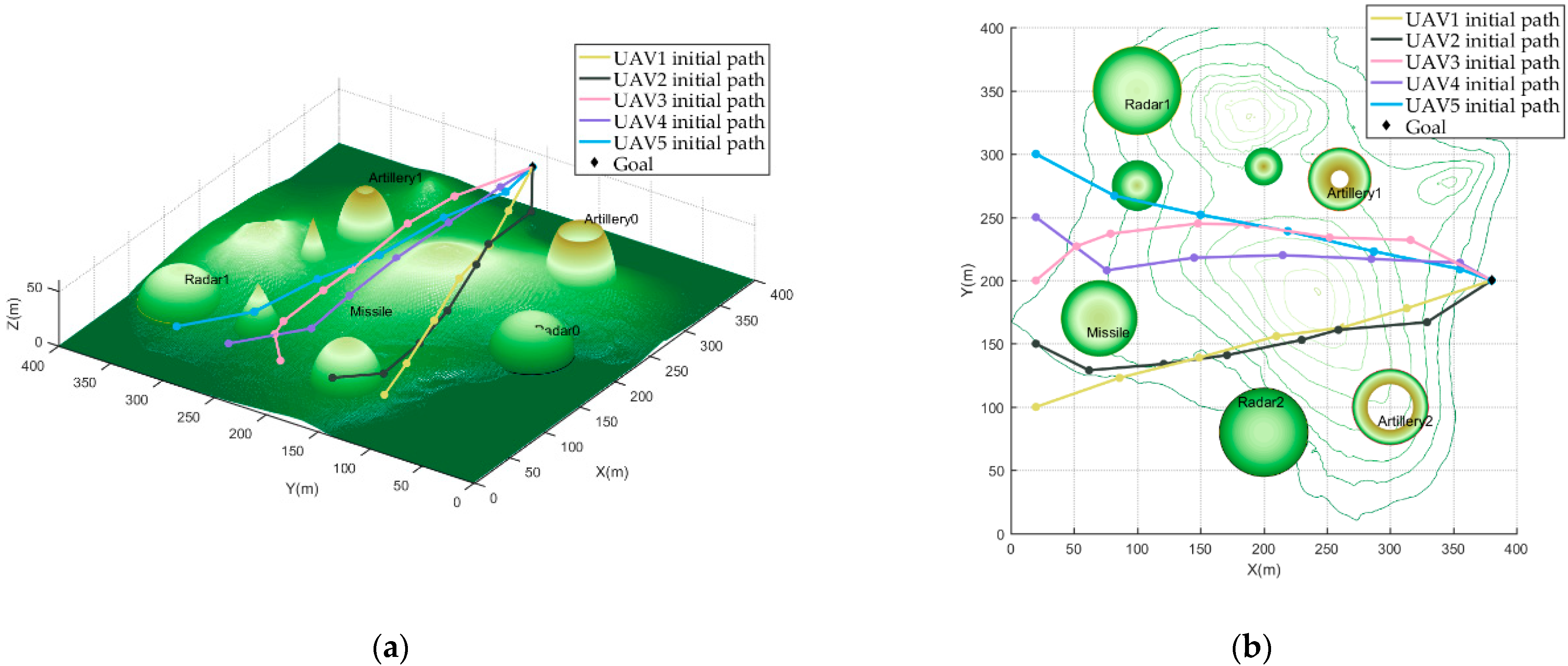
2.

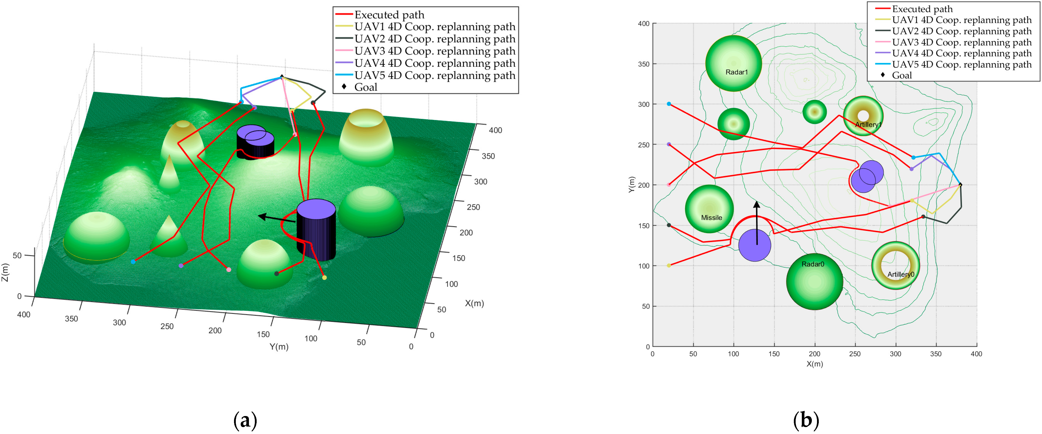
Complicated Scenario (Scenario 2). In this scenario, we set up five UAVs with the same performance. All UAVs take off from different starting nodes at the same time and arrive at the same goal. Figure 8 shows the planning environment of the Complicated Scenario, including radar, missiles, artilleries, no-fly towers, moving threats, and terrain threats based on elevation maps. Of these, sudden threats appear many times at different times, and their status is static or moving. In addition, a sudden threat group (simulating the possible local minimum traps in the local collision avoidance planning) is set in Scenario 2. See

Table 2. Complicated Scenario.

Environmental information	Rader	Center		Radius
		1:(200, 80, 0) 2:(100, 350, 5)		35 35
	Missile	Center		Radius	Height
		(70, 170, 0)		30	60
	Artillery	Center		Radius	Height
		1:(300, 100, 0) 2:(260, 180, 0)		30 25	40 40
	No-fly Tower	Center		Radius	Height
		1:(200, 290, 10) 2:(100, 275, 10)		15 20	50 40
	Sudden moving threat	Center (t = 4.7s)	Speed	Moving direction	Appearing time
		(126, 125, 0)	3 m/s	Positive direction of Y-axis	t = 4.7 s
	Sudden threats group	Center	Radius	Height	Appearing time
		1:(260, 205, 0) 2:(270, 215, 0)	15 15	50 50	t = 16.5 s
UAVs		Start position		Goal position	Speed
	UAV 1	(20, 100, 40)		(380, 200, 50)	15 m/s
	UAV 2	(20, 150, 40)
	UAV 3 UAV 4 UAV 5	(20, 200, 40) (20, 250, 40) (20, 300, 40)

for the relevant parameters of the Complicated Scenario.

4.2. Scenario 1: Normal Scenario

In Scenario 1, the relevant parameters of the HAPF are set as follows: the attractive potential field coefficient is $k_{att}=8$ and the repulsive potential field coefficient is $k_{rep}=30$. The influence distance of obstacle threat is ${\rho }_o=20 \mathrm{m}$, the unit time step is $t=0.01 \mathrm{s}$, and the adjustment factor is $n=0.7$. The maximum steering angle is ${\varphi }_{\max }={60}^{°}$ and the maximum climbing/diving angle is ${\gamma }_{\max }={35}^{°}$. The generating node of the attractive potential field is the path node [157,296,50]. Figure 2 shows the 4D cooperative path (i.e., the generation path of the initial cooperative planning layer) when the UAV does not detect the moving threat. Figure 3, Figure 4, Figure 5 and Figure 6 show the collision avoidance path of the UAV at different times after detecting the moving threat (i.e., the generation path of local collision avoidance planning layer). The 4D dynamic cooperative replanning path of the UAV is shown in Figure 7 (i.e., the generation path of the cooperative planning layer).

Table 3. Relevant parameters of 4D cooperative replanning after avoiding sudden threats.

	Current Position	Unexecuted Path	Speed	ETA	${\mathit{l}}_{\mathit{c}\mathit{o}}$
UAV1	[177.88, 101.08, 38.88]	225.46	19.915	11.32	243.36
UAV2	[177.53, 184.60, 41.92]	209.83	18.534	11.32	226.49
UAV3	[157, 296, 50]	244.42	20	12.22	244.42

shows the shortest cooperation time for 4D cooperative replanning. See

Table 4. The deviation ratio between the actual path length obtained by the 4D cooperative path algorithm and $l_{\mathrm{co}}$.

	Expected 4D Path Length	Actual 4D Path Length	Deviation
UAV 1	243.36	244.85	0.61%
UAV 2	226.49	226.37	0.05%
UAV 3	244.42	244.42	0

for the deviation ratio between the actual path length obtained by the 4D cooperative path algorithm and $l_{\mathrm{co}}$.

It can be seen in Figure 3, Figure 4, Figure 5 and Figure 6 that, under the guidance of the HPAF algorithm of the local anti-collision planning layer, UAV3 is able to evade sudden moving threats. It should be noted that the path of UAV2 in Figure 6 shows that the moving threat could involve a collision. However, HAPF is an online planning algorithm. Each time a collision avoidance path in a unit time step is planned, the UAV flies along the planned path. When UAV3 has flown for 6 s, it reaches the path node with coordinates [147.6170, 326.0181, 49.2858]. When $t=6 \mathrm{s}$, the path node avoids the moving threat, so there is no collision. Finally, after 7.59 s of flight, UAV3 reaches the sub-target node; that is, the preplanned path node [157, 296, 50]. When $t=7.59 \mathrm{s}$, UAV3 has completed the avoidance of the moving threats. While UAV 2 evades the sudden moving threat, other UAVs fly along the initial cooperative path.

At this point, the 4D cooperative planning layer comes into play. It can be seen in Table 3 that the shortest cooperation time is 12.22 s. Based on this, the $l_{\mathrm{co}}$ of each UAV can be obtained to ensure time coordination. It can be seen in Figure 7 that after HAPF is used to circumvent the sudden moving threat, the proposed algorithm uses the DPRRT* algorithm in the cooperative planning layer to replan the 4D cooperative path of all UAVs. Due to the constraints of spatial cooperation, the cooperative paths of the three UAVs do not collide, thus meeting the requirements of spatial cooperation. At the same time, combining the deviation between the expected cooperation path and the actual planned cooperation path in Table 4, it can be seen that the deviation percentage is within the allowable range, meeting the time cooperation requirements.

Based on the above simulation results and analysis, the proposed algorithm is able to realize the planning of a 4D dynamic cooperative path of all UAVs in the Normal Scenario, thus proving the effectiveness of the proposed algorithm.

4.3. Scenario 2: Complicated Scenario

In Scenario 2, the relevant parameters of the HAPF are set as follows: the attractive potential field coefficient is $k_{att}=8$ and the repulsive potential field coefficient is $k_{rep}=30$. The influence distance of obstacle threat is ${\rho }_o=20 \mathrm{m}$, the unit time step is $t=0.01 \mathrm{s}$, and the adjustment factor is $n=0.7$. The maximum steering angle is ${\varphi }_{\max }={60}^{°}$ and the maximum climbing/diving angle is ${\gamma }_{\max }={35}^{°}$. It can be seen in Table 2 that we have set up two kinds of sudden threats at different times. The first one is a mobile threat and the second one is a static threat group simulating a local minimum trap. Figure 8, Figure 9 and Figure 10 show the pre-planned 4D coordination path and the satisfaction of 4D coordination constraints of the path when t = 0 s. 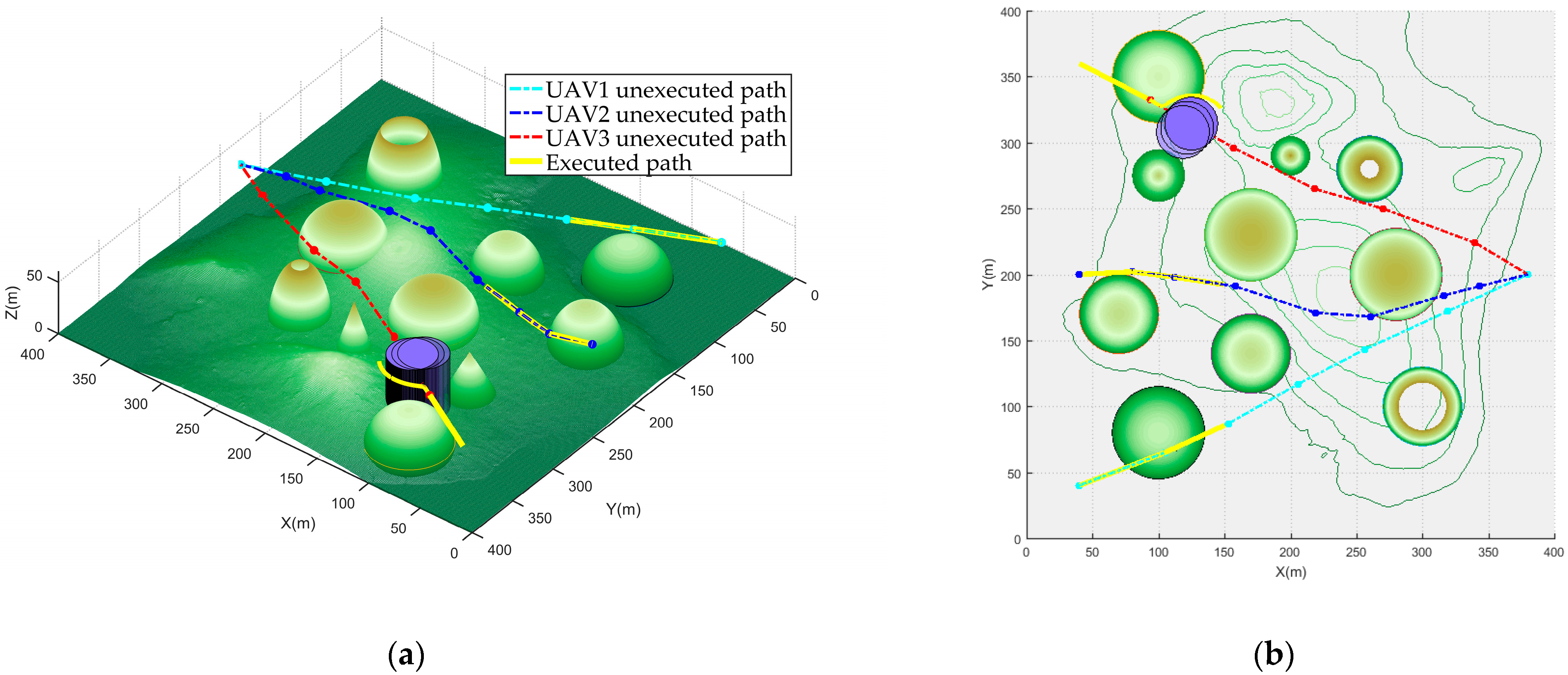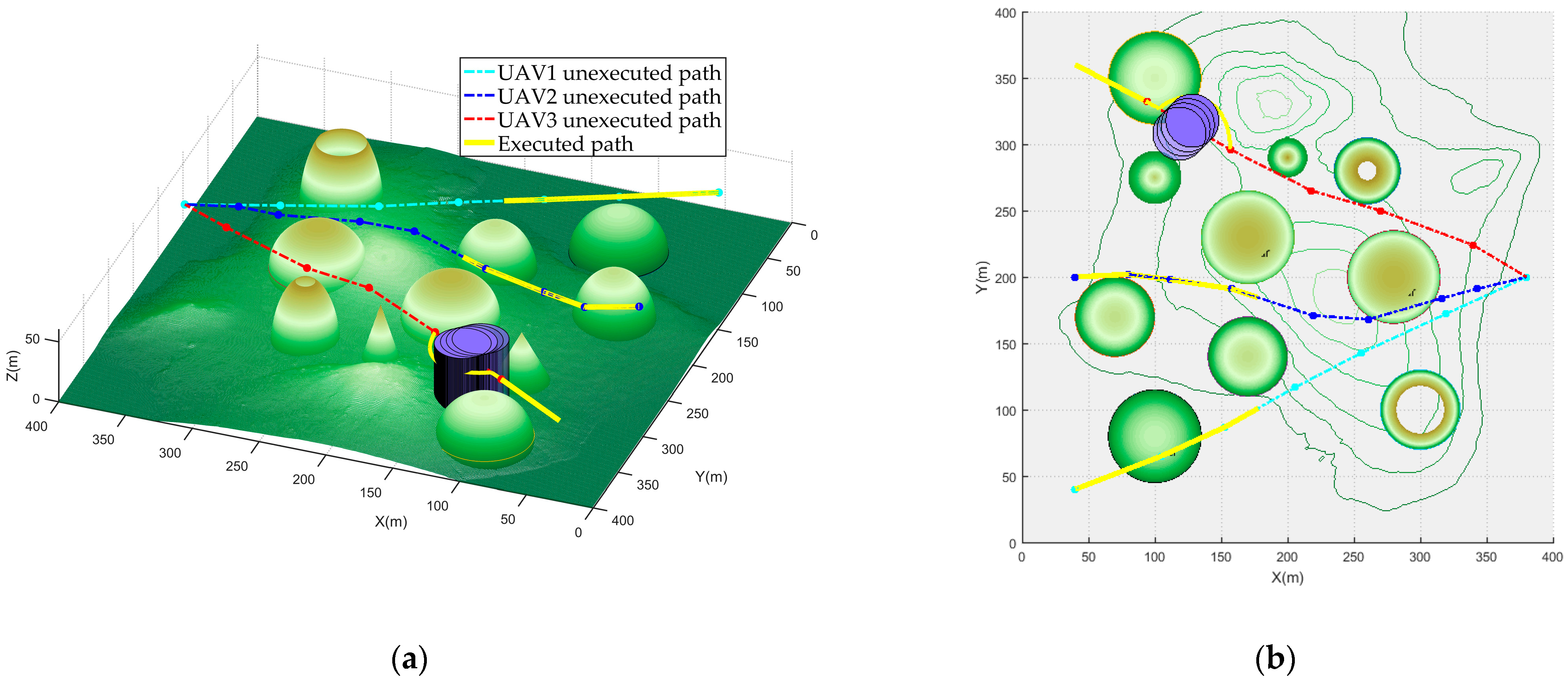Figure 11 shows the local collision avoidance planning path of some UAVs and the 4D cooperative replanning path of all UAVs after the first sudden moving threat. Figure 12 and Figure 13 show the satisfaction of 4D cooperative constraints of the pre-planned path based on the current planning space. 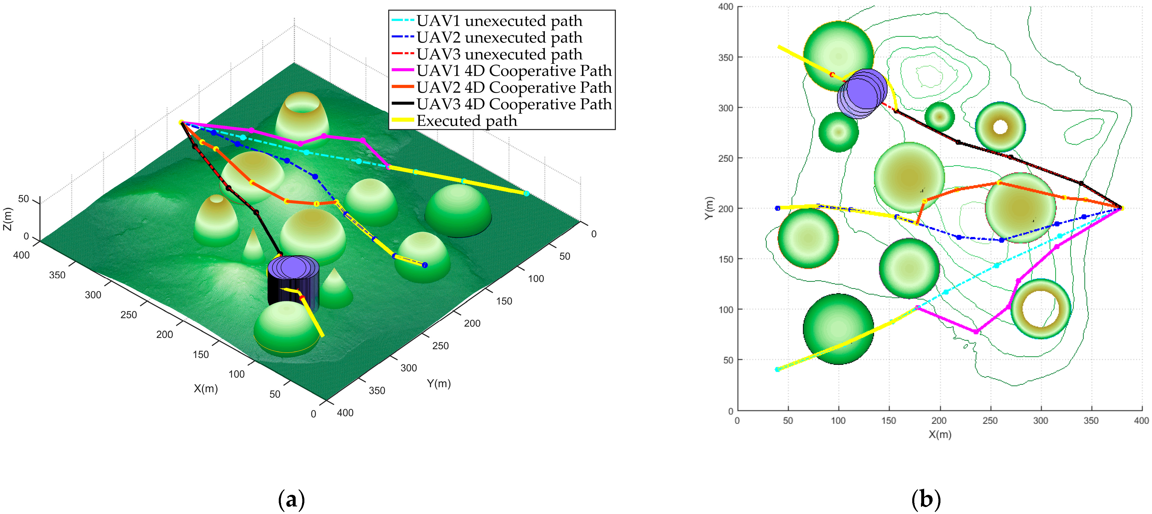Figure 14 shows the dynamic planning path of the proposed algorithm when affected by the sudden threat group for the second time, including local collision avoidance planning and 4D cooperative path replanning. 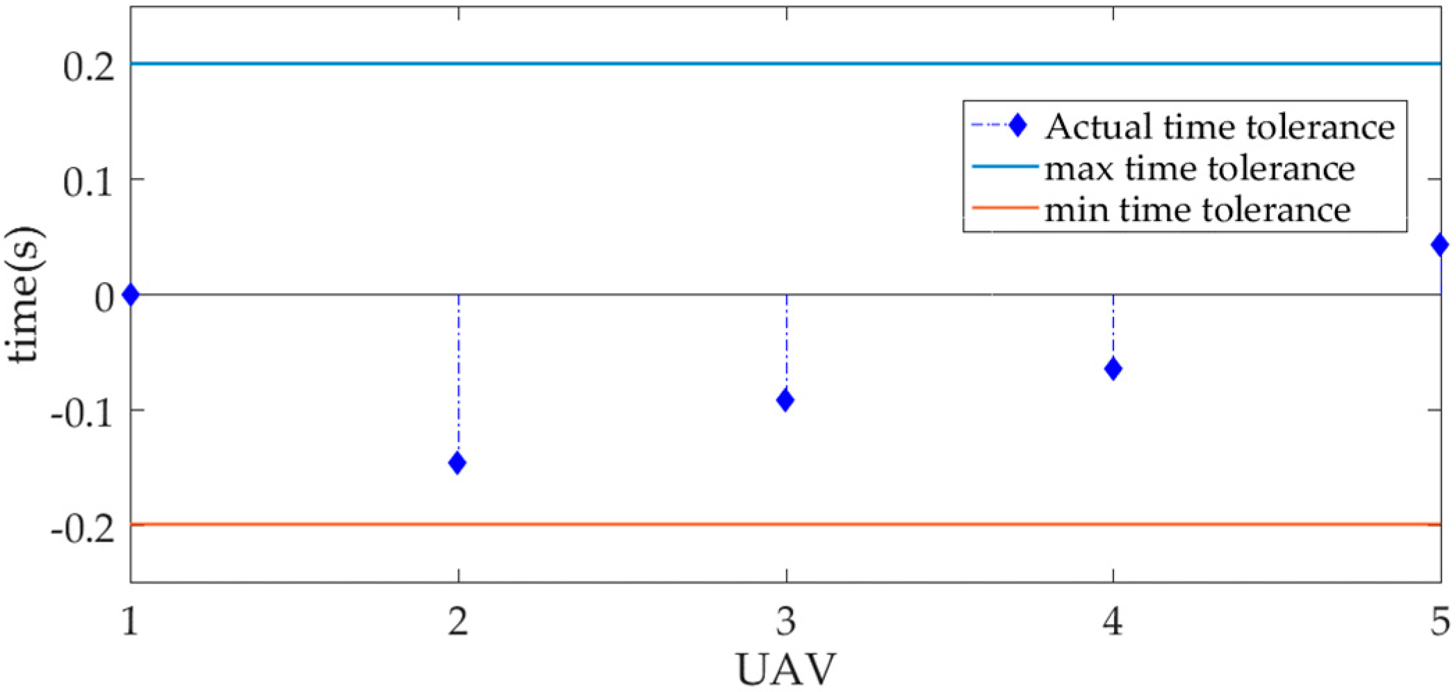Figure 15 and Figure 16 show the satisfaction of 4D cooperative constraints of the planned path.

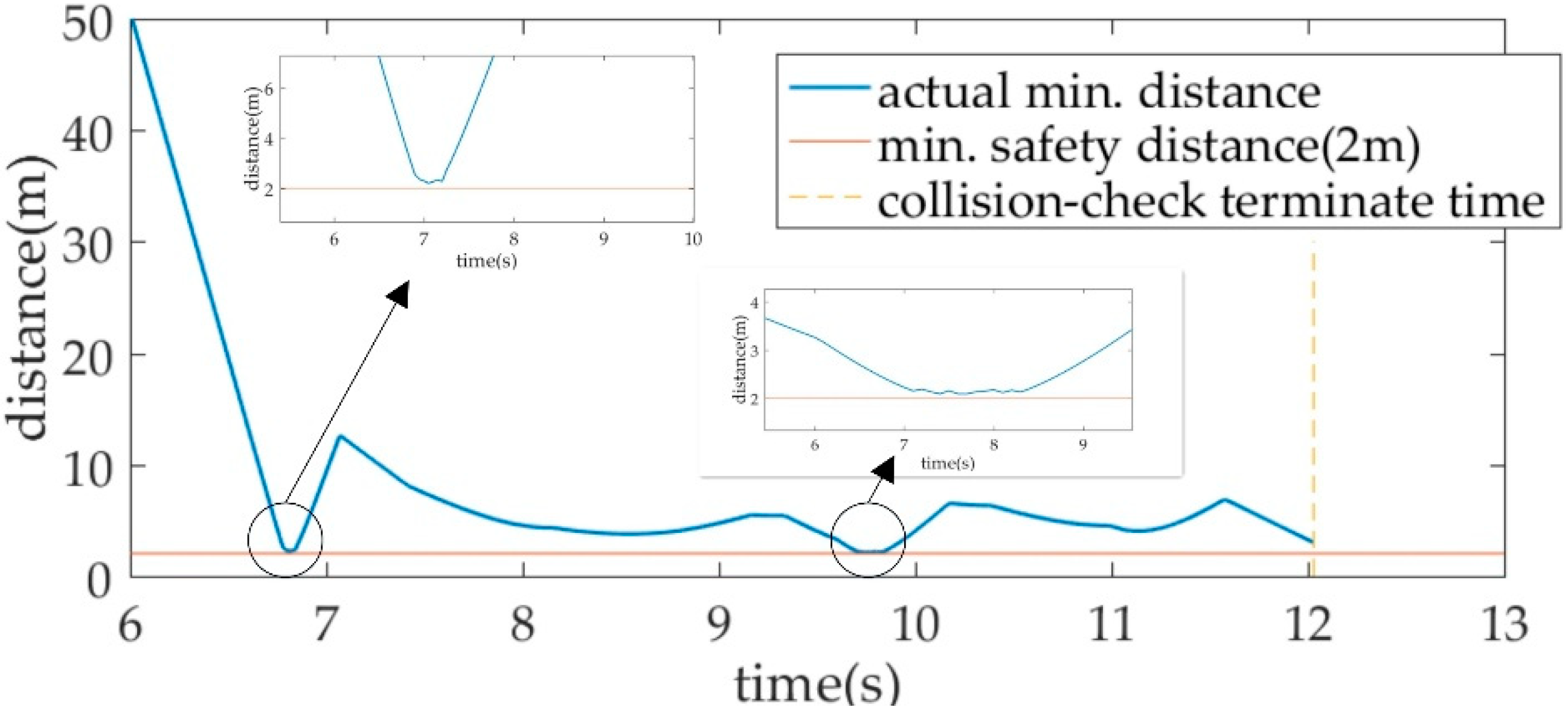
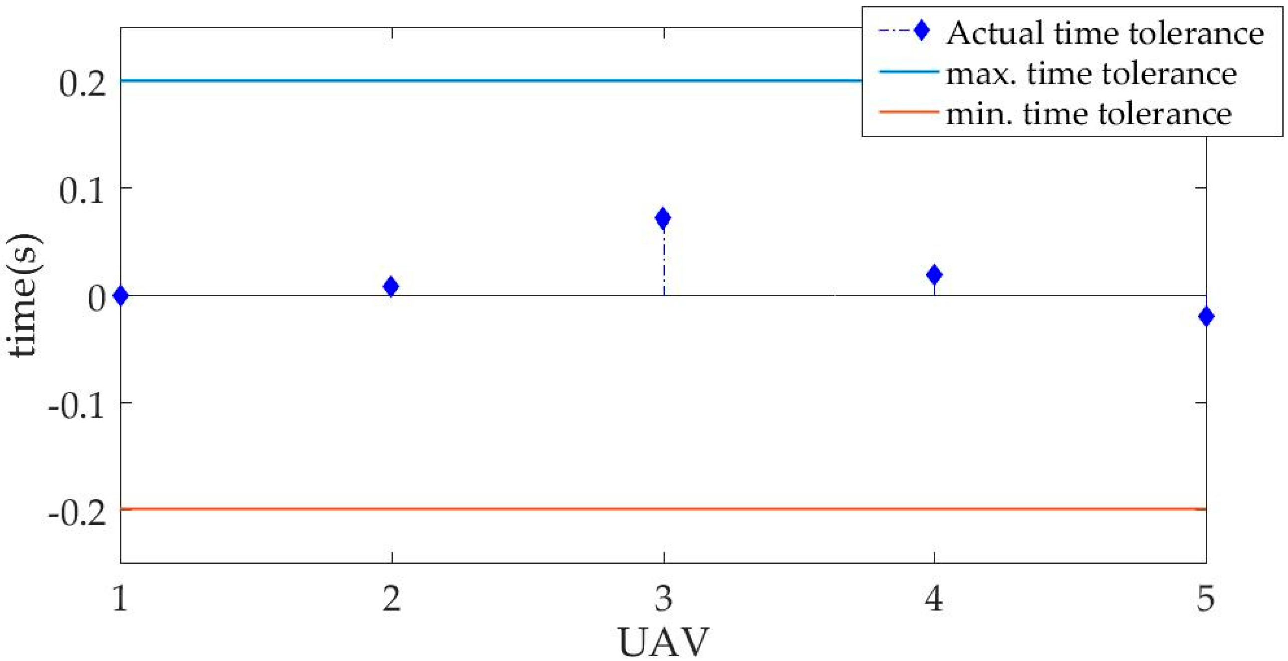
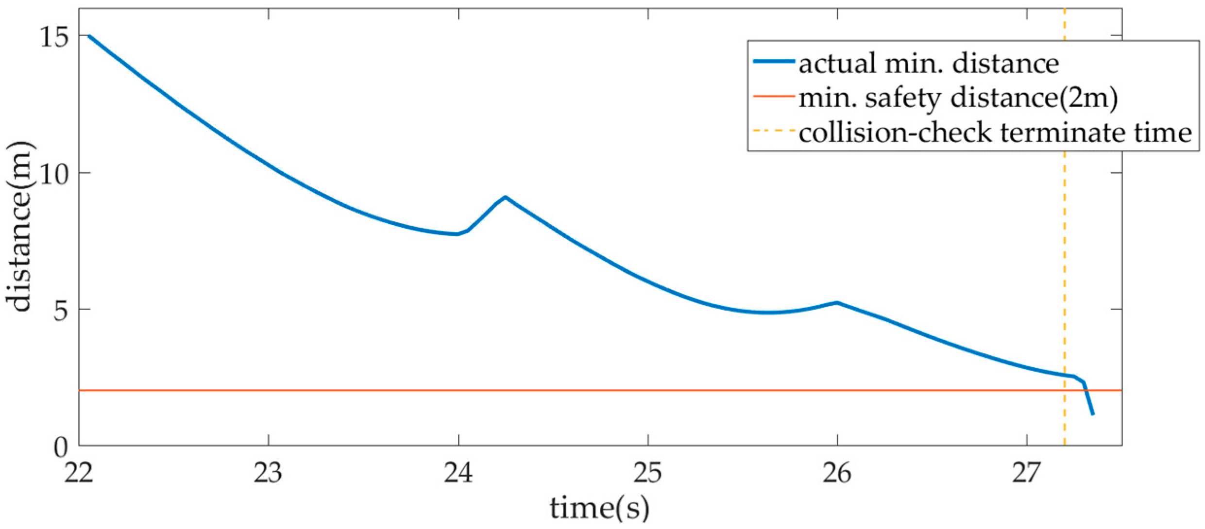
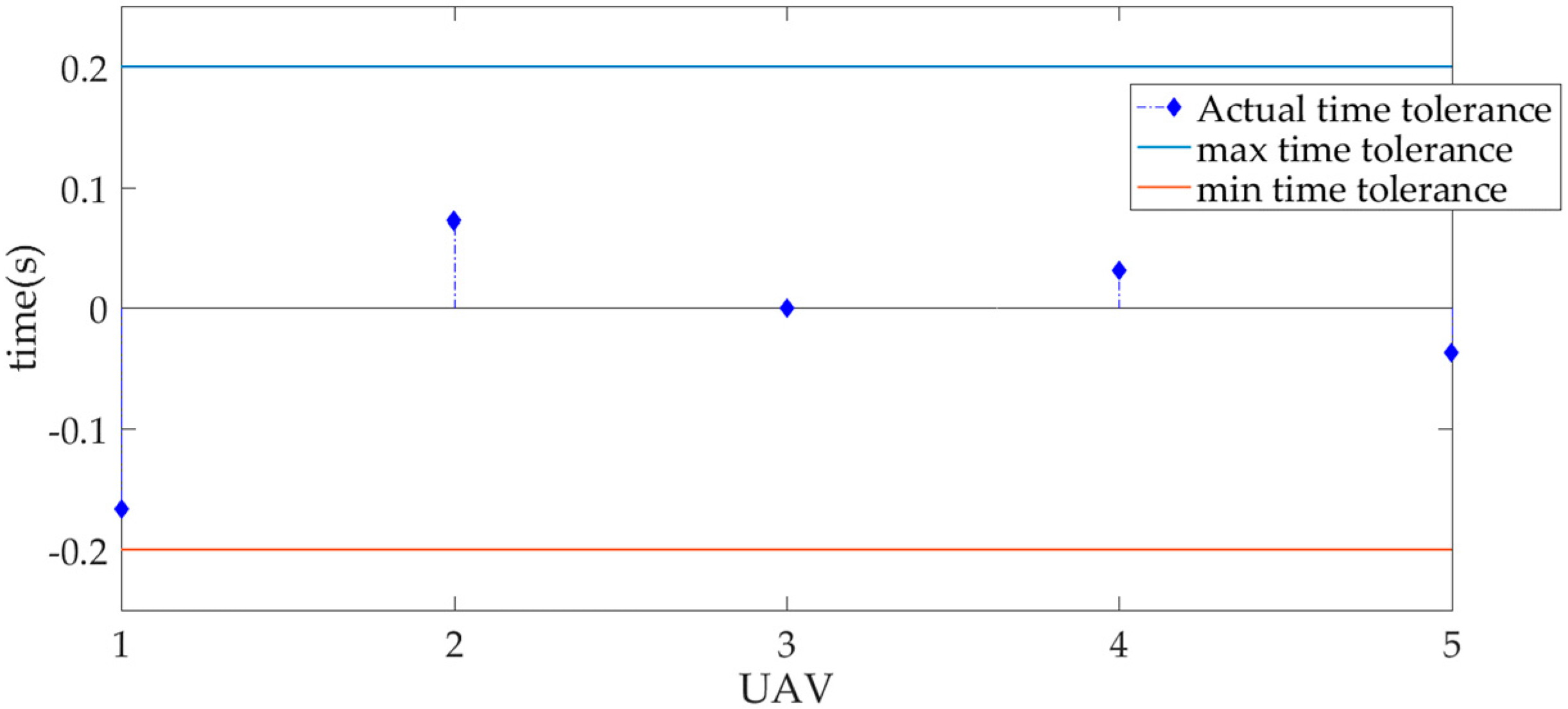
It can be seen in Figure 9 that the shortest distance between each pair of UAVs at the same time is larger than the minimum safety distance (2 m) we set, so it can be shown that the pre-planned path meets the space constraints in 4D cooperative constraints. At the same time, it can be seen in Figure 10 that the ETA tolerance of the five UAVs executing the pre-planned path is within 0.2 s, i.e., they meet the time cooperative constraints.

When t = 4.7 s, a sudden moving threat appears in the planning space for the first time. Compared with Scenario 1, the sudden moving threat in Scenario 2 will affect two UAVs at the same time, which is more complex. The collision avoidance planning of two UAVs based on the HAPF algorithm will be executed online at the same time, and the planning needs to avoid sudden threats while preventing conflicts with other UAVs. Figure 11 shows the path of local collision-checking planning and 4D cooperative replanning. It can be seen in Figure 11 and Figure 12a that UAV1 and UAV2 can avoid threats in the environment during local collision-checking planning, and two UAVs can maintain a safe distance to avoid conflicts. After completing local collision-checking planning, all UAVs need to conduct cooperative path replanning to meet 4D coordination constraints. It can be seen in Figure 12b that the cooperative replanning path can meet the spatial constraints. In addition, Figure 13 proves that the collaborative replanning path can meet the time coordination constraints.

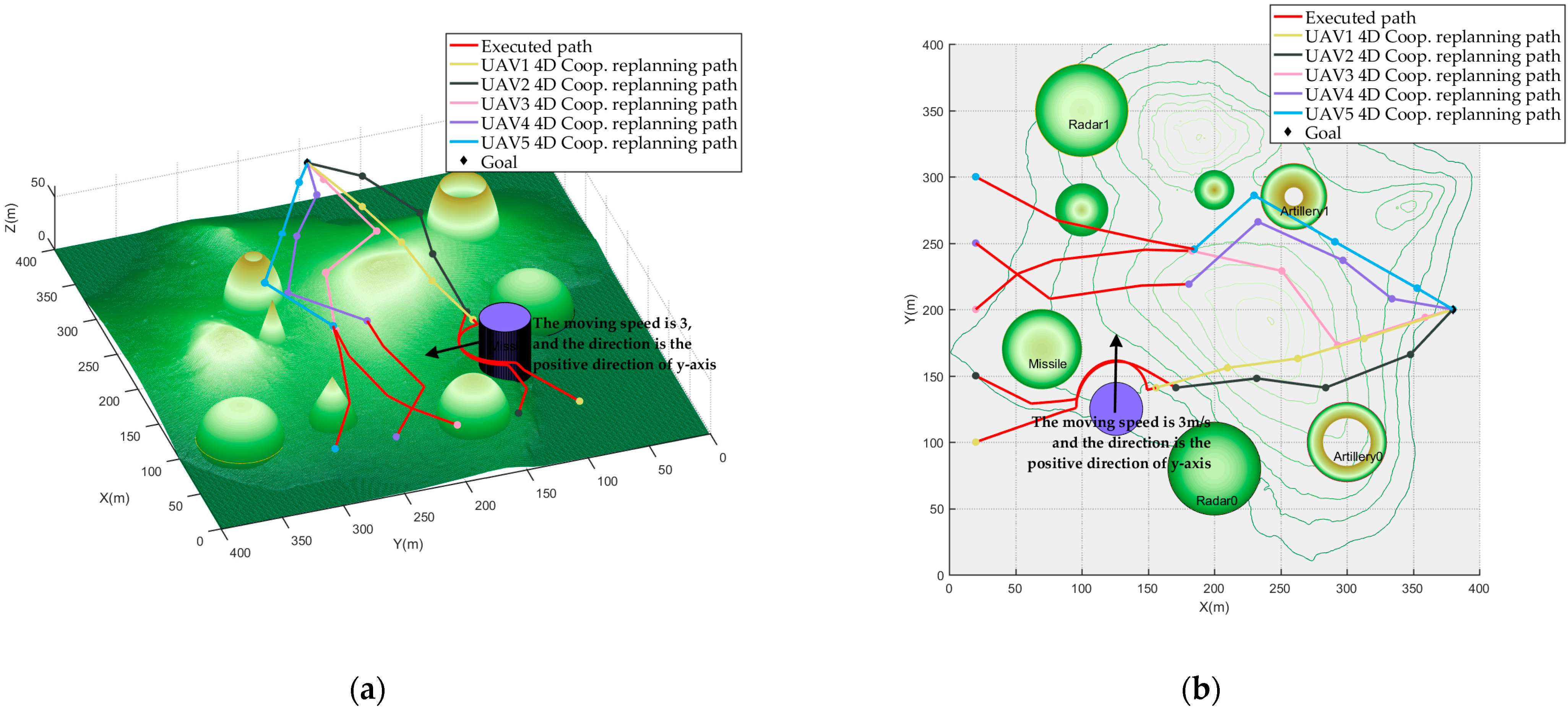
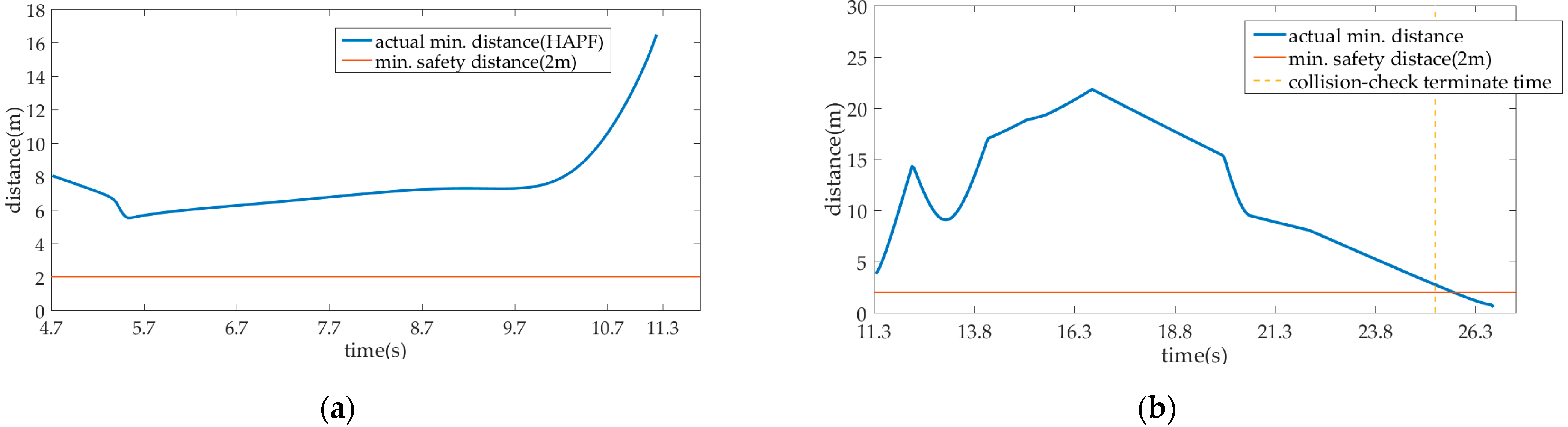
Similarly, when t = 16.5 s, the planning space changes for the second time. We set up a group of sudden threats to simulate the planning of escaping from the local minimum trap in local collision avoidance. It can be seen in Figure 14 that after being affected by threats, UAV3 can plan the path to escape from the local minimum. After that, all UAVs continue to replan the 4D cooperative path, so that all UAVs can reach the goal without conflict. It can be seen in Figure 15 and Figure 16 that the second cooperative path replanning can plan the path satisfying 4D cooperative constraints for all UAVs.

Based on the above analysis, we can prove that the proposed algorithm can still complete the dynamic, 4D cooperative path planning in complex scenarios. Therefore, we prove the effectiveness of the proposed algorithm in different scenarios.

4.4. Comparison and Algorithm Performance Analysis

In this section, we compare the 4D cooperative path planning layer (DPRRT* algorithm) and local collision avoidance planning layer (HAPF algorithm) of the 4D dynamic cooperative path planning algorithm with some related algorithms. On the basis of comparison, the performance of the 4D dynamic cooperative path planning algorithm is analyzed.

4.4.1. Comparative Simulation and Performance Analysis of Cooperative Path Planning Layer

The DPRRT* algorithm is a decoupled cooperative planning algorithm. The generation of the cooperative path can be divided into two stages; namely, the planning sequence sequencing and the single machine cooperative path planning. At the same time, it should be noted that the existing priority planning algorithms and their derivative algorithms have not involved in-depth research on the 4D cooperative path planning problem. Therefore, in order to eliminate the impact of considering both time and space cooperation constraints on the performance of the algorithm, we uniformly set the cooperation constraints that the path needs to meet in terms of 4D cooperation constraints in comparison with related algorithms to more accurately compare and analyze the performance of the DPRRT* algorithm. In the context of the scenario of cooperative path planning based on the decoupling method, we introduced the prioritized A* algorithm [31], the traditional priority planning algorithm (RPP) [26], and the coupling degree-based heuristic prioritized planning algorithm (CDH-PP) [46] for comparison.

This simulation compares the two types of mission scenarios mentioned in Section 4.2 and Section 4.3. To fully analyze the performance of the DPRRT* algorithm in both the Normal Scenario and the Complicated Scenario, four algorithms are used for 4D cooperative path planning of three groups of UAVs with different numbers, where the number of UAVs is set as {2,4,6}. In the two scenarios, the starting and goal nodes of all UAVs are randomly generated in the planning space and 30 random problem situations are generated for each scenario.

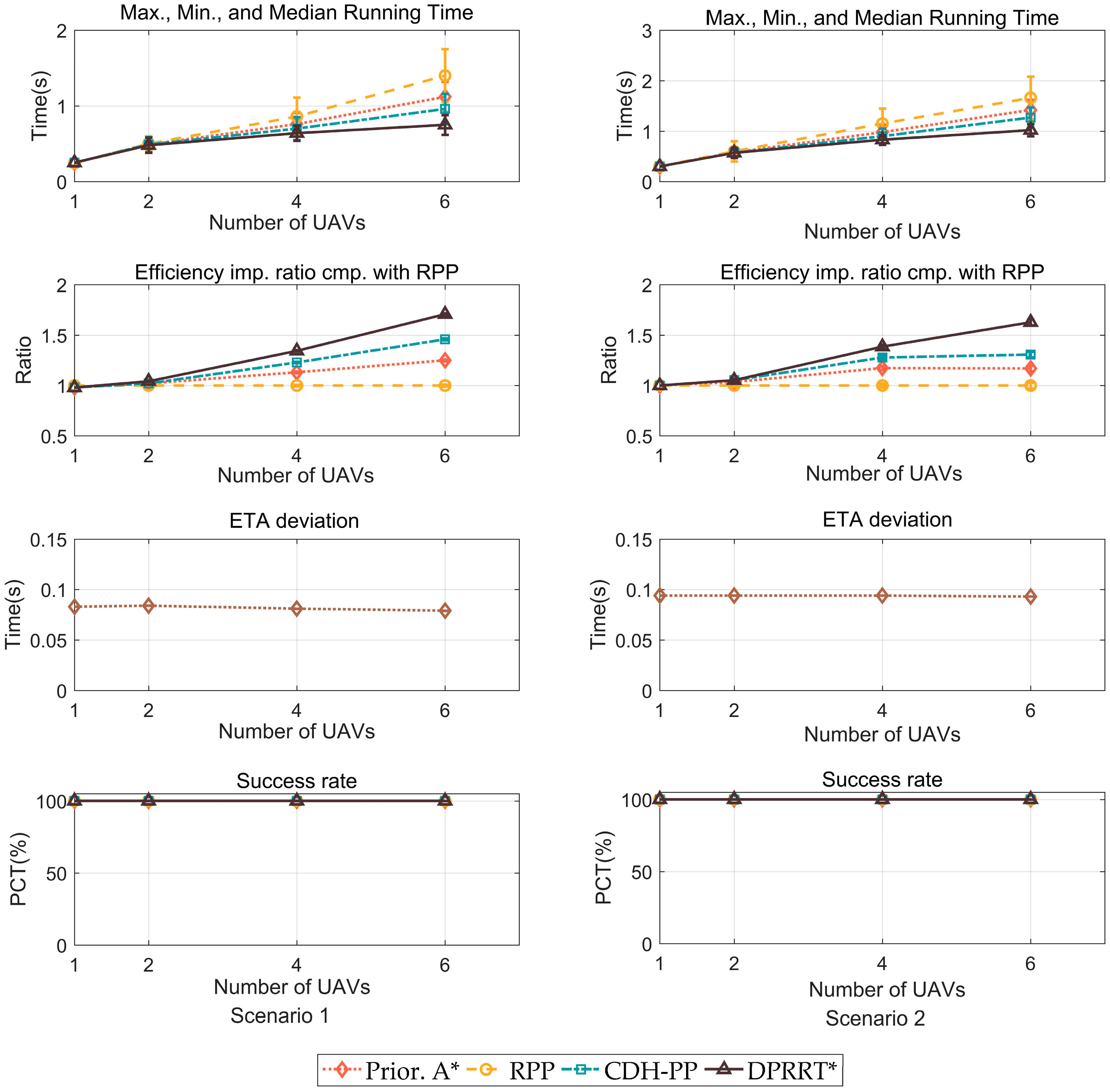
The characteristics of the four comparisons are as follows:

• The longest running time, the shortest running time, and the median running time of the algorithm (analyzing the computational efficiency and robustness of the algorithm).
• Compared with the RPP algorithm (the single UAV planning layer uses the RRT* algorithm based on 4D constraints), the acceleration ratio is used to evaluate the impact of different heuristic priority ranking strategies or different underlying algorithms on the cooperative planning algorithm. The formula for calculating the acceleration ratio is $\frac{t_i^{RPP}}{t_i^{ALG}}$. Where $t_i^{RPP}$ represents the running time of the RPP algorithm and $t_i^{ALG}$ represents the running time of the comparison algorithm.
• The ETA time difference is used to evaluate the quality of the path planned by the algorithm. The calculation formula is $t_{\max ETA}^{ALG}-t_{\min ETA}^{ALG}$, where $t_{\max ETA}^{ALG}$ represents the maximum flight time of the planned path of the four algorithms and $t_{\min ETA}^{ALG}$ represents the minimum flight time of the planned path of the four algorithms.
• The success rate can be used to verify the effectiveness of the algorithm.

The comparison results of the four algorithms are shown in Figure 17.

It can be seen from the comparison of the running time in Figure 17 that the median running time of the DPRRT* algorithm is the shortest and the difference between the maximum and minimum running times is relatively small. In addition, DPRRT* has the highest acceleration ratio. The comparison results of DPRRT* with RPP and CDH-PP prove that the heuristic prioritization strategy based on time cooperation constraints is more reasonable, efficient, and robust. In addition, the running time comparison between DPRRT* and Prioritized A* proves that the single machine cooperative path planning algorithm based on 4DRRT* in DPRRT* has higher efficiency and stability than the A* algorithm. Since the four algorithms have the ability to find the optimal solution, there is little difference in the ETA. In addition, the four algorithms are decoupled algorithms, so they all have a high success rate.

4.4.2. Comparative Simulation and Performance Analysis of the Local Anti-Collision Planning Layer

We simulated the three improvements of the HAPF algorithm and compared them to the classic APF algorithm.

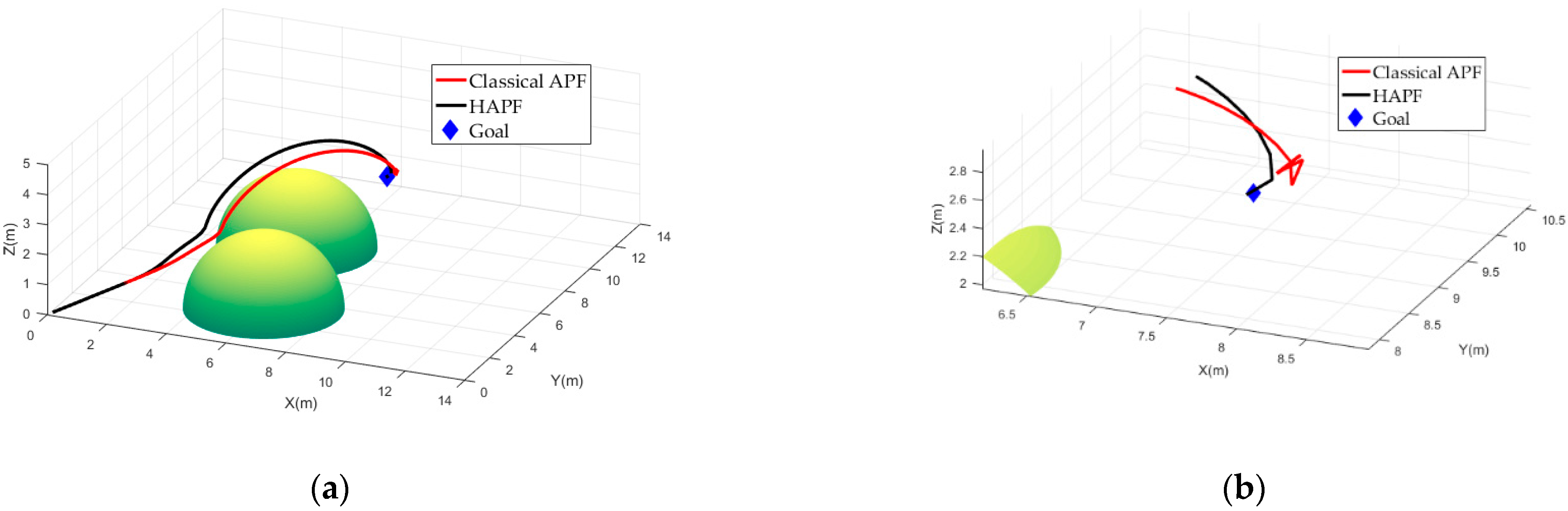
In the simulation, an improved repulsive force function was added to solve the problem of the unreachability of the target. The traditional artificial potential field was compared with HAPF in the path collision avoidance planning of obstacles near the target.

In order to verify the effectiveness of the algorithm and ensure the optimal performance of the traditional algorithm, the traditional algorithm was simulated using the best parameters. At the same time, in order to intuitively show the superiority of the improved potential field function, this simulation used the radar threat as the environment model for verification. The potential field parameters of the HAPF algorithm are $k_{att}=8$, $k_{rep}=30$, ${\rho }_o=2 \mathrm{k}\mathrm{m}$, $l=0.2 \mathrm{k}\mathrm{m}$, and $n=0.7$. According to the simulation data, the generation node of the repulsion potential field corresponding to the last path node is [7.1654, 9.9636, 1.9927] km. The relative distance between this node and the target node is 1.0541 km, which is less than the obstacle influence distance, so obstacle threat near the target node is extant.

Figure 18 shows the comparison between the two algorithms. It can be seen in Figure 18 that HAPF reaches the target node, while the traditional potential field method has the problem of target unreachability. The relative distances between different path nodes and target nodes of UAVs in the two algorithms are recorded separately. It can be seen that when there is an obstacle threat near the target, the traditional artificial potential field method oscillates near the target node and cannot reach the target node. The improved potential field method is able to reach the target node, which shows that the improved algorithm can solve the problem of the unreachable target.

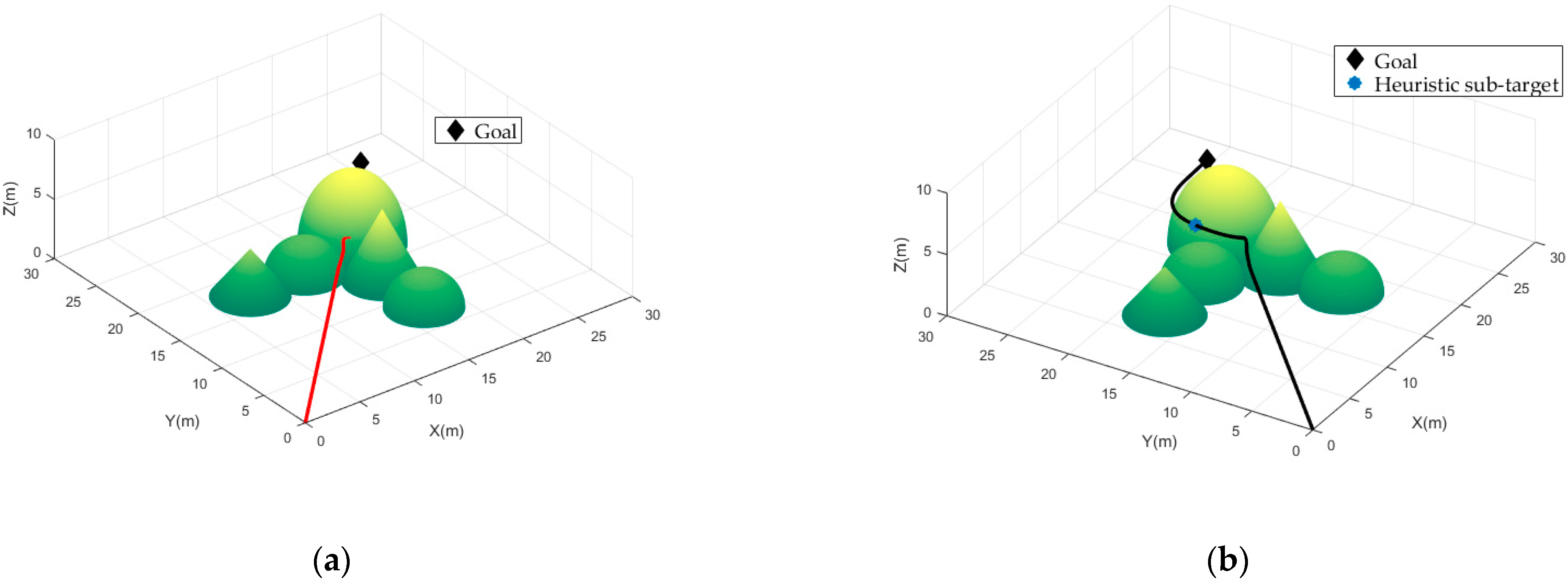
Regarding the problem of the traditional artificial potential field method easily falling into the local minimum, this paper proposes a strategy to set heuristic target nodes in order to escape the local minimum. In the simulation, HAPF is compared with the traditional artificial potential field method. The potential field parameters are set as $k_{att}=8$, $k_{rep}=20$, $n=0.7$, ${\rho }_o=2 \mathrm{k}\mathrm{m}$, and $l=0.2 \mathrm{k}\mathrm{m}$ in the simulation. The starting node of the UAV is [0,0,0] km, and the goal is [22,22,5] km.

In order to fully verify the effectiveness of the algorithm, five combined obstacles with different obstacle threats are established in the simulation, and the five obstacles constitute the local minimum area. Figure 19a shows the traditional artificial potential field method and Figure 19b shows the HAPF algorithm. It can be seen in Figure 19a that when the UAV reaches the path node [13.9930, 14.5990, 4.7578] km, it falls into the local minimum value and oscillates back and forth near it, unable to escape it. In Figure 19b after the UAV has been trapped in the local minimum area, it successfully escapes and finally flies to the target node due to the guidance of heuristic sub-target nodes. The virtual spherical radius of the selected sub-target node is 3.1370 km, and the heuristic sub-target node coordinates are [13.1161, 17.5908, 4.9435] km. According to Figure 19 and the simulation data, after adding heuristic sub-target nodes, the UAV is able to escape the local minimum region, which solves the problem of the traditional potential field model easily falling into the local minimum.

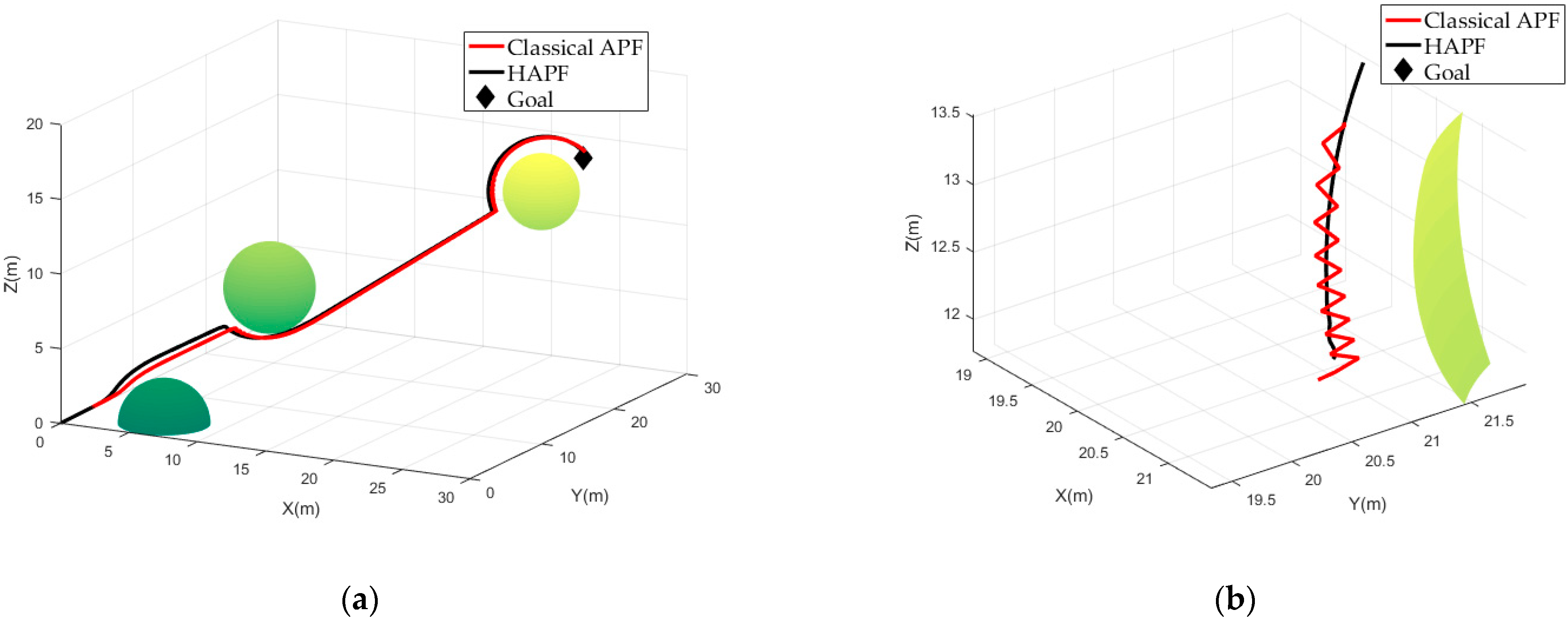
In this paper, regarding the problem of the improved potential field easily generating local path vibrations when avoiding obstacles and planning trajectory collision avoidance, a memory resultant force strategy was proposed to improve this problem. In the simulation, by comparing the traditional artificial method with the potential field method, the effect of resultant force memory on improving the local vibration is verified. In the simulation, the potential field simulation parameters are set as $k_{att}=8$, $k_{rep}=20$, $n=0.7$, ${\rho }_o=2 \mathrm{k}\mathrm{m}$, and $l=0.2 \mathrm{k}\mathrm{m}$. In the HAPF algorithm with a memory factor, the value of the memory factor is set to ${\lambda }_1=0.7$ and ${\lambda }_2=0.3$. Figure 20 simulates the flight path of the two algorithms.

It can be seen in Figure 20 that the UAV flight path was significantly improved after adding the memory resultant force without the local path oscillation. It can also be seen in Figure 20 that after adding the memory resultant force, the variations of resultant force angle between adjacent path nodes of the UAV become significantly smaller and there is no significant angle oscillation. This shows that the introduction of this strategy satisfies the flight constraints of UAVs, does not cause large angle changes between adjacent path nodes, makes the flight path smoother, and is suitable for the collision avoidance trajectory planning of UAVs.

5. Conclusions and Future Work

In this paper, a 4D dynamic cooperative path planning algorithm is proposed to solve the cooperative path planning problem under the 4D cooperative constraints of multiple UAVs. Each UAV shares the same arrival time. There is no conflict between them and they are able to successfully implement threat avoidance. The algorithm proposed in this paper adopts a hierarchical architecture; namely, a 4D cooperative path planning layer and a local anti-collision planning layer. First, the DPRRT* algorithm was used to complete the 4D cooperative preplanning based on the initially known environment before UAV flights. Later, if a UAV encounters sudden threats while in flight, the HAPF algorithm of the local anti-collision planning layer is used to avoid these sudden threats. Simultaneously, UAVs not affected by sudden threats continue to fly along their planned paths. It should be noted that the 4D cooperation constraint cannot be satisfied after the sudden threat avoidance. Therefore, after the sudden threat avoidance has been completed, the DPRRT* algorithm in the 4D cooperative path planning layer is used to replan the 4D cooperative path. Whenever a new threat appears, local obstacle avoidance planning and 4D coordinated path replanning of the threat are required until all UAVs reach the target at the same time. The simulation and comparison experiments show that the proposed algorithm is able to plan a cooperative path, thus satisfying the 4D cooperative constraints for UAVs, and the algorithm has high efficiency, stability, and robustness.

In future work, we plan to extend the proposed algorithm to other application levels; that is, we aim to use multiple UAVs for the actual experimental verification of the proposed algorithm. In addition, considering that the swarm intelligence cooperation composed of a large number of UAVs may be a hot topic in the near future, we plan to improve the algorithm proposed in this paper and explore a 4D cooperative planning algorithm that can be synchronized, so that the algorithm is able to achieve efficient and robust cooperative path planning for 50 or even 100 UAVs.