Sensitivity of LiDAR Parameters to Aboveground Biomass in Winter Spelt

Abstract

Information about the current biomass state of crops is important to evaluate whether the growth conditions are adequate in terms of water and nutrient supply to determine if there is need to react to diseases and to predict the expected yield. Passive optical Unmanned Aerial Vehicle (UAV)-based sensors such as RGB or multispectral cameras are able to sense the canopy surface and record, e.g., chlorophyll-related plant characteristics, which are often indirectly correlated to aboveground biomass. However, direct measurements of the plant structure can be provided by LiDAR systems. In this study, different LiDAR-based parameters are evaluated according to their relationship to aboveground fresh and dry biomass (AGB) for a winter spelt experimental field in Dahmsdorf, Brandenburg, Germany. The parameters crop height, gap fraction, and LiDAR intensity are analyzed according to their individual correlation with AGB, and also a multiparameter analysis using the Ordinary Least Squares Regression (OLS) is performed. Results indicate high absolute correlations of AGB with gap fraction and crop height (−0.82 and 0.77 for wet and −0.70 and 0.66 for dry AGB, respectively), whereas intensity needs further calibration or processing before it can be adequately used to estimate AGB (−0.27 and 0.22 for wet and dry AGB, respectively). An important outcome of this study is that the combined utilization of all LiDAR parameters via an OLS analysis results in less accurate AGB estimation than with gap fraction or crop height alone. Moreover, future AGB states in June and July were able to be estimated from May LiDAR parameters with high accuracy, indicating stable spatial patterns in crop characteristics over time.

1. Introduction

In agriculture, aboveground biomass (AGB) is an important parameter for assessing the crop health status, the water and nutrient supply, and the effects of agricultural management practices [1]. Recently, it has gained importance due to agro-ecosystems becoming potential sources of carbon sequestration as well as carbon-dioxide-neutral energy sources by cultivating biofuels [2].

Most published studies are utilizing passive optical systems to monitor AGB at the field scale or beyond. Reference [3] recently reviewed the potentials of Unmanned Aerial Vehicles (UAV) to retrieve AGB for the special case of grasslands. There are two main approach groups [4]: (i) The application of structure-from-motion, i.e., photogrammetric stereo RGB imagery to generate digital surface maps of crop height to relate these to AGB [5,6,7]. Here, the acquisition timing during the day on the height measurements from stereo imaging impacts the results due to shadowing and ground pixel visibility effects with different solar angles [5]. Similar results were reported for differences in the plant development stages and cultivars [6]. To improve stereo-based AGB estimates, Ref. [8] calculated the sum of pixel values in a crop surface map without soil background to include volumetric information. (ii) The application of plant spectral properties does not provide a plant height or structure information, but it does provide characteristics about the canopy chlorophyll status [9]. As these denote plant vitality, they are typically correlated with AGB. e.g., [10] evaluated image texture features and spectral vegetation indices to estimate AGB for winter wheat at different growth stages. Especially, the combination of spectral indices with image texture such as variance, entropy, data range, homogeneity, second moment, dissimilarity, contrast, or correlation was able to improve the results significantly. Similar results were obtained for other cultivars [11,12,13]. Ref. [14] used hyperspectral vegetation indices as well as red-edge position and shape parameters to estimate biomass. The authors found a combination of vegetation indices and red-edge parameters as well as multiple regression methods to be more accurate than single linear regression of the independent variables. For both approach groups, machine learning techniques are widely applied [8,15].

In contrast, the three-dimensional structure of plants can be obtained by light detection and ranging (LiDAR) systems to enable direct AGB observations. Those active optical sensors have been utilized mainly to gain forest biomass estimates [16], while in agricultural ecosystems, mainly terrestrial laser scanning techniques were applied [17,18,19]. UAV-borne LiDAR observations for AGB estimation are more flexible and concise and provide multiangular 3D point clouds without platform-related shadow effects. Ref. [20] analyzed the relationships of total fresh biomass measurements with LiDAR crop height during different nitrogen treatment levels. Similarly, Ref. [21] used LiDAR crop height estimates and a stepwise multiple regression to estimate AGB. Ref. [22] investigated the benefits of fusing LiDAR and multispectral data for predicting sugarcane AGB. While their fusion results did not perform significantly better than the single source observations, they found that LiDAR was performing slightly better than multispectral imagery later in the season. However, most LiDAR-based biomass estimates as well as stereo-optical methods make use of the plant height information only. A rare exception is [23], which used a layered gap fraction method of [24] to retrieve a dimensionless three-dimensional profile index and a regression to in situ measurements. Ref. [24] used LiDAR intensity to classify vegetation and soil points, while [25] distinguished between active and no-longer-functioning, senescent vegetation. Ref. [26] used LiDAR intensity to derive links to properties of the biochemistry of vegetation such as nitrogen status and chlorophyll concentrations. An important milestone in the estimation of crop traits, including AGB, is the very recent publication by [27]. The authors provided detailed information about advanced methods to retrieve LiDAR parameters, e.g., by a vertical distribution of the normalized point heights within each reference area to describe the vertical structure of crops. Ref. [27] used the coefficient of determination and the root mean square error as statistical measures to evaluate the potential of the UAV LiDAR metrics.

In this study, the LiDAR parameters height, point cloud gap fraction, and as the signal reflection intensity are evaluated for their relationship to fresh and dry aboveground biomass in winter spelt.

2. Materials and Methods

2.1. The Dahmsdorf Study Site

The Dahmsdorf study site is located close to the city of Müncheberg in the German federal state of Brandenburg. Geologically, this hummocky ground moraine landscape consists mainly of strongly sandy glacial till from ground moraine material and sandy, predominantly fine-grained, partly fine silty deposits caused by meltwater from Weichselian glaciation. From this originates a soil heterogeneity which can be regarded as an important driver for crop growth variability. The long-term average annual temperature at this site is 9.5 °C, with an average annual precipitation of 560 mm [28]. Here, a field experiment has been established to implement and test a new cropping system called patch cropping [29] and to analyze crop performance and technical challenges during management of small-scale and complex field geometries. Patch cropping is a potential measure to increase biodiversity and to reduce environmental impacts of agriculture [29,30].

For the delineation of management zones (patches) within the field, georeferenced data such as proximal sensed data sets of electrical bulk resistivity measured by the GEOPHILUS system [31] and indexes derived from a digital elevation model with 1 m resolution such as topographic wetness index [32] and slope angle classes were used. To avoid fragmented smaller zones and to generate larger meaningful segments, a superpixel algorithm-based tessellation with a size of approximately 600 m² from an aerial image was implemented [9]. Subsequently, an unsupervised Fuzzy c-means clustering algorithm with equal weighting of the input data delineated two zones [33]. As direct payments under Common Agricultural Policy require a minimum plot size of 0.3 ha, a merging procedure to generate connected patch structures with a minimum size of 0.3 ha was performed. Due to the complex geometries of the patch structures and the working widths used by the farmer, a manual simplification had to be carried out. The characteristics of the two cluster group classes in terms of soil and topographic attributes are listed in

Table A1. Mean values (and standard deviation) of topography and different soil attributes of the two cluster group classes.

Attributes	Cluster Group Class 1	Cluster Group Class 2
Total area	4.37 ha (62,0%)	2.70 ha (38.0%)
Electrical bulk resistivity (0–25 cm) (Ohm m)	390.3 (198.9)	827.5 (305.2)
<= 2 µm—Clay (%) *	1.77 (0.27)	1.41 (0.27)
>2 µm and <= 63 µm—Silt (%) *	21.73 (4.42)	14.15 (2.71)
>63 µm—Sand (%) *	76.50 (4.61)	84.44 (2.93)
Slope angle classes I	17.0%	29.8%
Slope angle classes II	49.7%	61.4%
Slope angle classes III	31.2%	8.3%
Slope angle classes IV	2.1%	0.5%
Slope angle classes V	-	-
Topographic wetness index	5.7 (1.25)	6.42 (1.47)

* Derived from 24 soil texture analysis points of the Ap horizon.

in Appendix A.

Two crop rotations were developed for each cluster group class according to their site potential (including winter spelt, buckwheat, rye, and lupine for cluster group class 1 and alfalfa-grass mixture, rye, and lupine for cluster group class 2). The cultivation of the field is under an organic farming scheme and does not include synthetic mineral fertilization or plant protection measures. In order to study the effects of the different cluster group classes in growing season 2021/2022, the field was split into a part with 7 alternating strips and the 2 retrieved management zone patches. The crops alfalfa-grass mixture and winter-spelt were cultivated. The field for winter spelt was plowed and prepared for sowing on 30 September 2021. The certified winter spelt was drilled on 11 October 2021. Weed control took place on 16 March 2022 using a tine harrow.

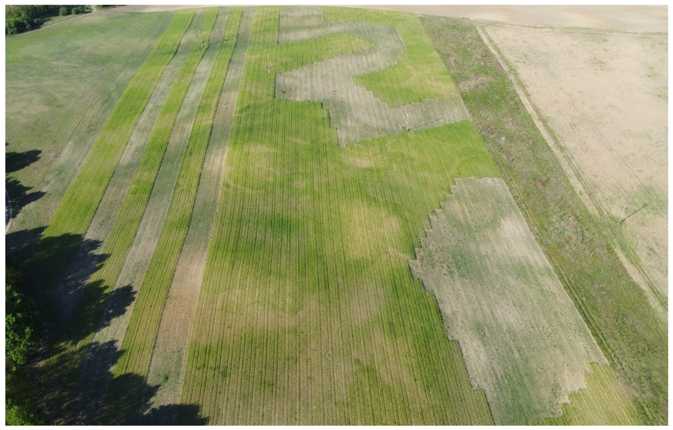
As the alfalfa-grass mixture was already harvested at the date of the UAV flight campaign, we focus in this study on the winter spelt fraction only. As is visible in Figure 1, topography and soil texture already push through a high variability in crop phenology in the winter spelt zone. To map this variability—measured as AGB—LiDAR parameters are evaluated.

2.2. Aboveground Biomass Sampling

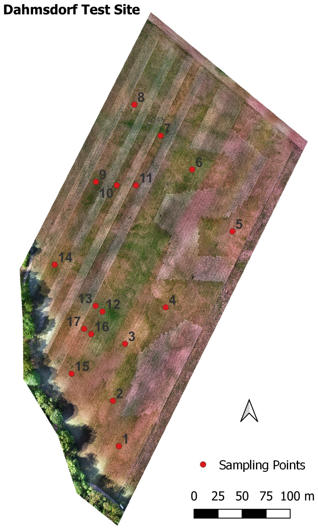
Wet and dry aboveground biomass was destructively sampled at 17 locations in the winter spelt cultivation in the Dahmsdorf site (see Figure 2). The spacing of individual seed rows within the population was 12.5 cm. The sample locations were selected to cover both the overall field as well as the full variability of the phenology. The samples were taken at three dates in the vegetation period with roughly one month interval, i.e., 10 May, 16 June, and 14 July 2022. Biomass was cut along a row of 100 cm and dried 48 h at 60 °C and is therefore given in g/m. Due to mechanical weed control and biomass cutting of plant material within the seed row, only weed-free plant material was sampled.

Four samples were taken per point. To relate those samples to the LiDAR parameters, the median values were calculated, and a 2 m buffer was applied to the LiDAR parameter maps to reduce small-scale heterogeneity. Moreover, the buffer reduces the impact of the invasive sampling, as the flights were performed after the in situ measurements.

2.3. UAV-Based Yellowscan Surveyor LiDAR

The UAV carrying the YellowScan^® Surveyor LiDAR (YellowScan, Saint-Clément-de-Rivière, France) is a DJI Matrice 600 (DJI, Shenzhen, China), equipped also with a DJI Zenmuse X5 RGB camera [34]. The LiDAR is based on the Velodyne VLP-16 Puck scanner (Velodyne, San Jose, USA) and the Applanix APX15 (Trimble Applanix, Richmond Hill, Canada) single board GNSS-Inertial solution. The 1.6 kg weight sensor sends out 300,000 rapid laser pulses (in 360°) per second and captures the returning signals with a precision of ~4 cm. The wavelength of the LiDAR is given with 903 nm, i.e., operating in the near infrared (NIR) spectrum.

The flight campaign took place on 18 May 2022. The Internal Measurement Unit (IMU) was calibrated by flying in forward, backward, and U-turn paths with strong acceleration and slowdown. The field of view was limited to 70° with maximum ±35° off-nadir point observations. The UAV was operating in an altitude of 55 m above ground with a ground speed of 18 km/h; one battery stop was necessary in between. The 10 flight paths were planned with an azimuth angle of 57° along the cultivation lines within the flight planning software DJI Ground Station Pro. This sampling scheme was selected to ensure adequate coverage and point density (see also [23]). An external Septentrio Altus NR3 (Septentrio, Leuven, Belgium) GNSS base station recorded >3 h GPS and GLONASS data.

After flight, the collected data were processed in Applanix’s POSPac (version 8.6) software, where a Smooth Best Estimated Trajectory (SBET) file was created. Afterwards, YellowScan’s CloudStation software was used to align the stripes of the flights for georeferencing. Corrections through GNSS offset (lever-arms), sensor angle (boresight), and GNSS postprocessing with precise position techniques were applied.

2.4. Extraction and Calculation of LiDAR Parameters

The software CloudCompare (version 2.11.1) was used to calculate the required LiDAR parameters from the calibrated point cloud. The LiDAR parameters crop height, gap fraction, and intensity were extracted at a grid size of 15 cm, resulting in high-resolution maps covering the multiple crop heterogeneities. The 15 cm grid was selected as a compromise between an adequate number of LiDAR points in a grid cell according to our observation scheme and the ability to generate a high-resolution map required by precision farming practices. The lowest point in the 15 cm grid cell defines the value for the minimum point map, whereas the highest point in the 15 cm grid cell defines the value for the maximum point map. To calculate the crop height ($CH$), the minimum points map was subtracted from the maximum points map.

The gap fraction ($GF$) is a measure of canopy density. It relates LiDAR point measurements reaching the ground through the canopy in relation to the total number of points including those that return from on top and within the canopy, resulting in the following equation:

$$GF=\frac{n_{ground}}{n}$$

(1)

where $n_{ground}$ is the number of points reaching the ground in the defined area, and $n$ is the total number of points (sum of ground points and off-ground points) in the same defined area. Therefore, it is necessary to separate the LiDAR dataset into ground and nonground points. This was achieved by Cloth Simulation Filtering (CSF) in CloudCompare [35].

The LiDAR intensity ($Int$) is recorded as the strength of the return signal of a laser beam. It depends not only on the composition of the reflecting surface objects, but also on range, angle, roughness, and moisture content [36]. The YellowScan Surveyor intensity values were not calibrated in this study, and an accuracy level information was not provided by the manufacturer. Without calibration, they are provided in terms of digital numbers (DN). Mean intensity values were transferred to the 15 cm grid.

2.5. Statistical Analysis

The LiDAR parameter maps at 15 cm resolution served as the basis to extract the average crop height, gap fraction, and intensity data of the AGB sampling locations—averaged for the 2 m buffer area. The resulting table was analyzed according to the individual relationships between the parameters. Here, the focus was set on the proportions of LiDAR parameters to wet and dry AGB in the May sampling campaign, which were the temporally closest to the UAV measurements. However, as biomass samples for June and July 2022 were also available, the continuity of AGB pattern were investigated in addition. The standard Pearson correlation coefficients were calculated between parameters.

Moreover, to identify the potential of multiple parameters to estimate AGB jointly, an ordinary least squares regression (OLS) was applied. With this approach, coefficients of linear regression equations were estimated, which describe the relationship between the multiple independent quantitative variables (LiDAR parameters) and a dependent variable (AGB). This is achieved by minimizing the sum of the squares of the differences between the observed dependent variable in the input dataset and the output of the linear function of the independent variable (see, e.g., [37]). After mean normalization of the variables, this also provides insights into the relative predictive skill of each dependent variable, i.e., providing their importance.

However, if two or more predictor variables are highly correlated, they will not provide unique information in the regression model. Therefore, multicollinearity needs to be considered. We performed a multicollinearity analysis for the LiDAR parameters crop height, gap fraction, and intensity with the variance inflation factor (VIF). VIF is based on an ordinary least squares regression analysis and quantifies the severity of multicollinearity. It provides a measure that clarifies how much the variance of an estimated regression coefficient is increased because of collinearity. The LiDAR parameter showing VIF greater than 5 can be removed without losing information.

3. Results

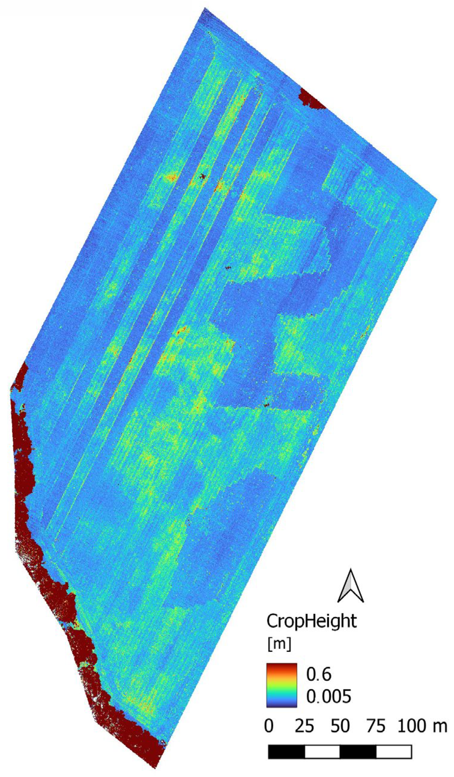
The retrieved LiDAR crop heights on the investigated patch crop field in Dahmsdorf are presented in Figure 3. Besides the trees and the phone line masts (three masts in the area of investigation), the patch crop structure clearly stands out. Particularly striking are the three stripes running parallel to each other and the jagged m-shaped area. Moreover, the machine lines and tracks visible in Figure 1 can be observed in the high-resolution crop height map. This justifies the application of the 2 m buffer for the correlation analysis, as those could affect the relationship. Within the winter spelt zones, variability in crop height has been recorded. The values range between 10 cm in and nearby the cultivation tracks to 60 cm within areas of high fertility.

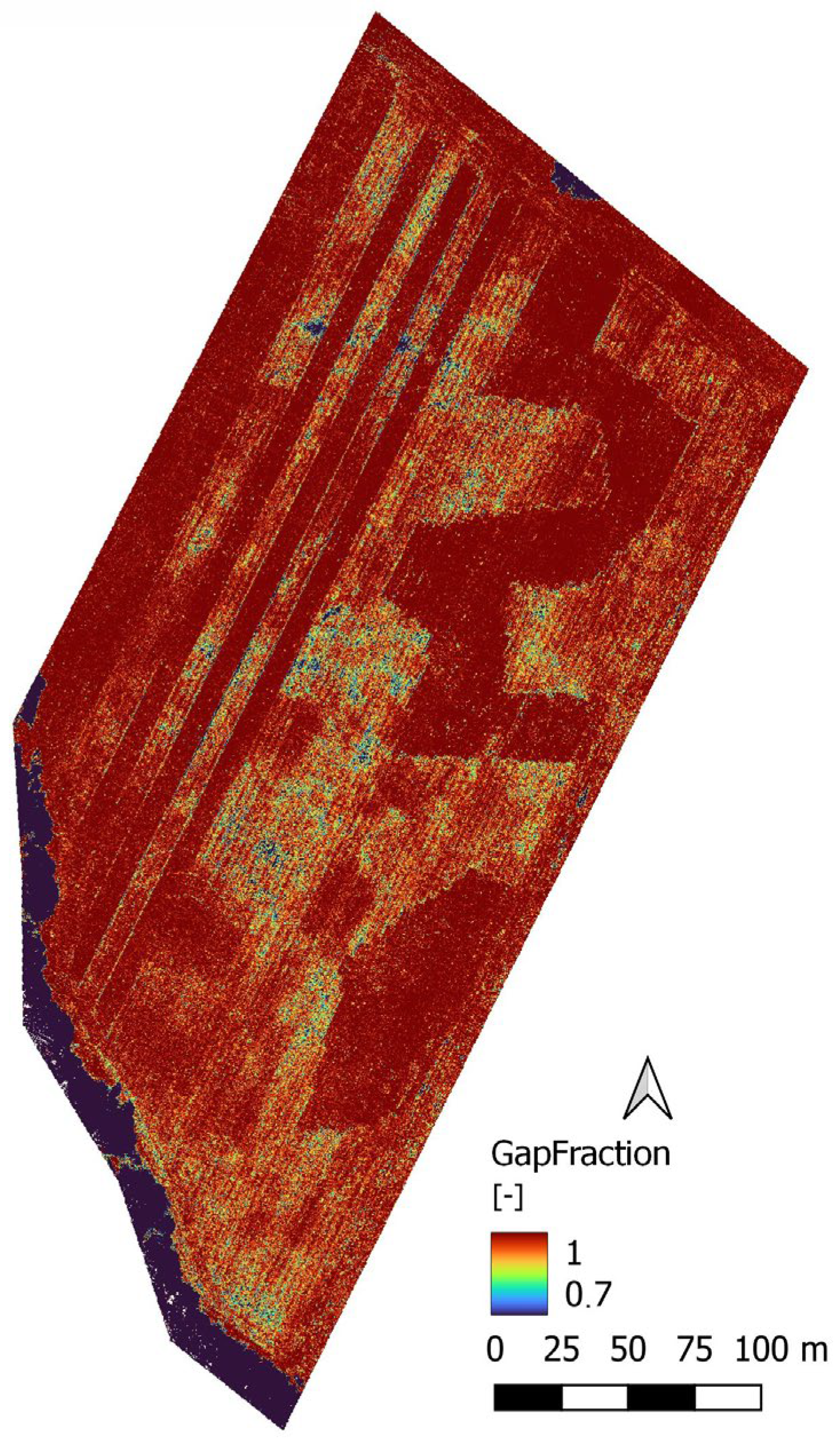
In Figure 4, the LiDAR gap fraction as a result of the point separation into ground and off-ground points by the CSF is presented. Clear variability in the winter spelt subfield conditions is visible. Especially in the already-harvested regions, the laser returns originate mainly from near the soil surface level, resulting in a gap fraction close to 1. In the regions where the winter spelt is still cultivated, the values vary between 0.5 and 1, whereas the general gap fraction level is high. This is a typical situation in upright standing vegetation such as cereals and observations with UAV LiDAR. Here, only a few small areas have this low gap fraction level of 0.5, and most values are above 0.8.

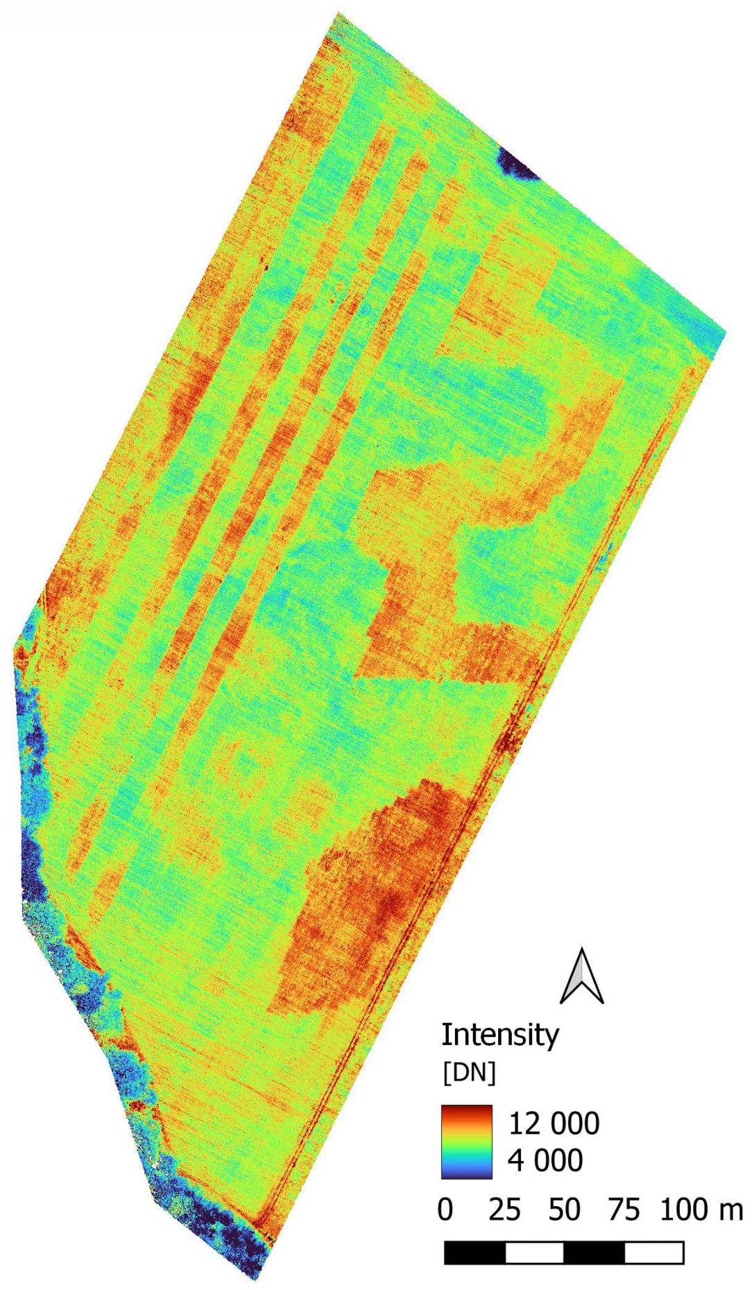
The mapping result of the LiDAR intensity is presented in Figure 5. The harvested areas provide higher intensity levels (above 10,000 DN) than the winter spelt areas. The latter are characterized by a decent variability ranging between 5000 and 10,000. Striped artifacts are visible in the final map orthogonal to the flight and cultivation direction.

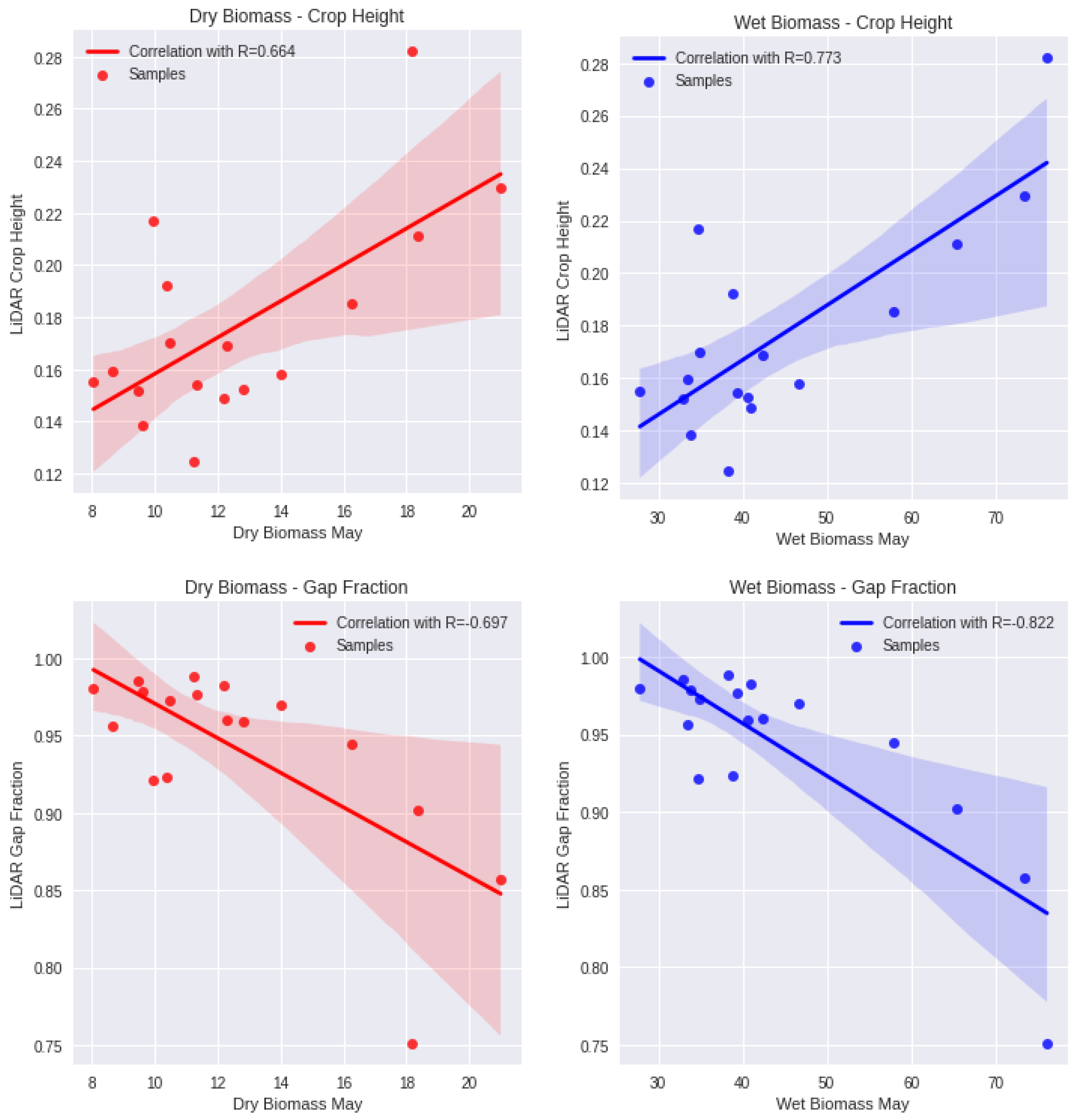
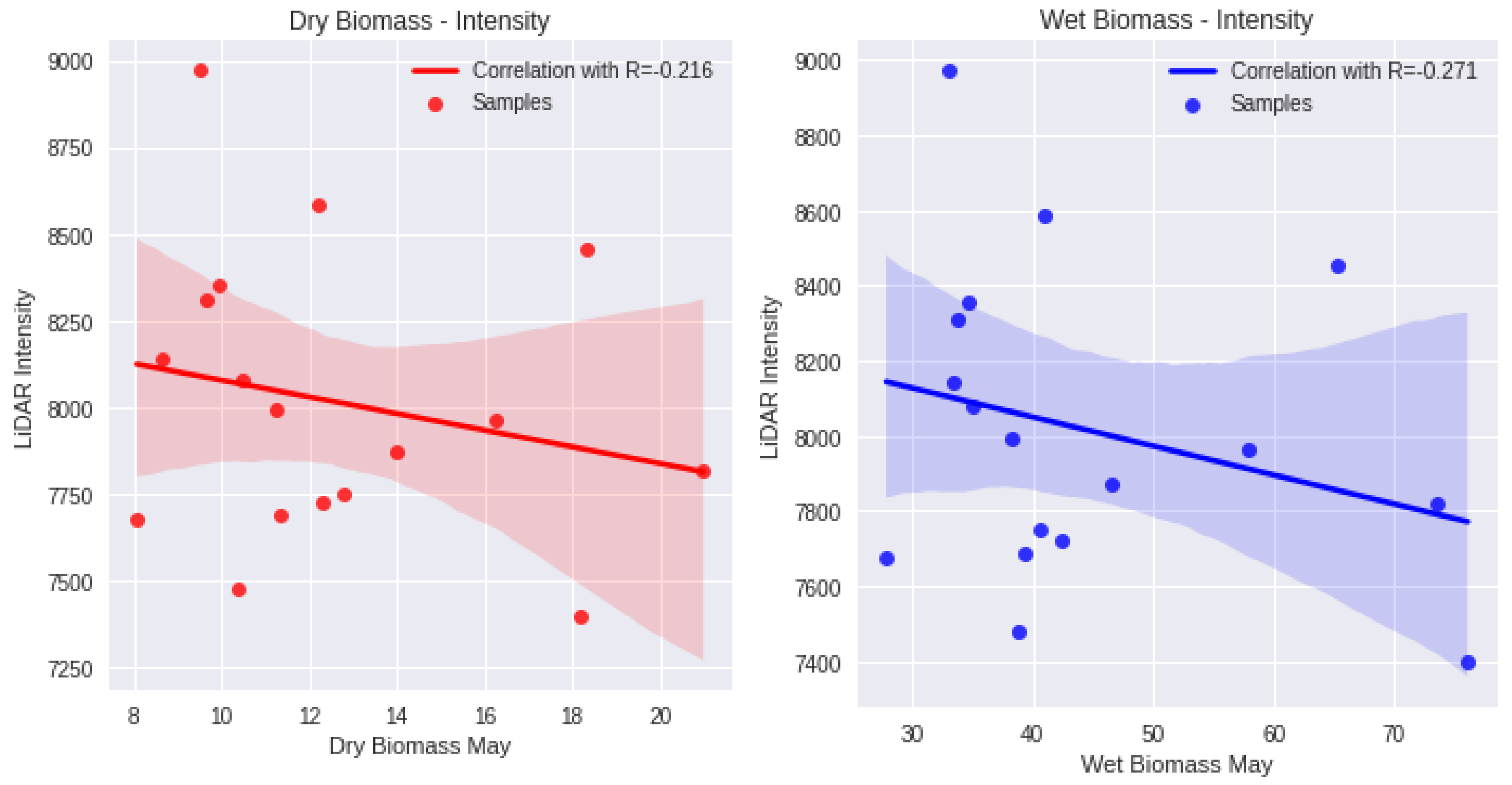
Correlations were calculated between the LiDAR parameters and the AGB data sampled in May 2022 at the 17 predefined points (see Figure 6). Here, AGB differs between dry and wet vegetation conditions. We found positive relationships to crop height with R = 0.664 (dry) and R = 0.773 (wet). The uncertainties are higher at lower AGB magnitudes. The highest absolute correlation coefficients were found with gap fraction but with an inverse relationship. The results are given with R = −0.697 (dry) and R = −0.822 (wet). The relationship of AGB with LiDAR intensity is also negative, but relatively weak with R = −0.216 (dry) and R = −0.271 (wet). According to the p-value statistics, the correlations of AGB to crop height and gap fraction are significant; the ones to intensity are not.

The OLS results after normalization for wet AGB are given with:

$$Wet Biomass May=-0.1517\ast C{H}_n-0.9981\ast G{F}_n+0.0791\ast I{n}_n$$

(2)

providing an R² of 0.682, while the intercept is negligible. The corresponding wet AGB is estimated by the OLS with:

$$Dry Biomass May=-0.0399\ast C{H}_n-0.7648\ast G{F}_n+0.0759\ast I{n}_n$$

(3)

providing an R² of 0.490. Additionally, here, the intercept is negligible. For both situations, the relationship of normalized AGB to the normalized gap fraction provides the highest (in this case negative) coefficients. For wet biomass, the coefficient is −0.9981, i.e., it is already suitable to use this parameter alone to estimate wet AGB. The other parameters contain less predictive power here.

To exclude multicollinearity, the VIFs were calculated. The factors for the LiDAR parameters crop height, gap fraction, and intensity are given with 11.10, 11.91, and 1.26, respectively. This indicates that crop height or gap fraction can be removed without losing information, whereas intensity cannot be removed without losing information. I.e., crop height and gap fraction are highly collinear.

4. Discussion

The maps of crop height, gap fraction, and intensity in Figure 3, Figure 4 and Figure 5 provide interesting spatial detail and certain variability in the winter spelt phenology. As we are focusing in this study on the relative relationships between the LiDAR parameters and the two AGB measurement types, absolute accuracy of these parameters is not important.

The crop height records from UAV LiDAR (Figure 3) are similar to those of [23], who obtained an R² of 0.78 and an RMSE of 3.4 cm. They showed, for another cereal crop (winter wheat), an underestimation of crop height, with its relatively open and upright structure allowing the laser beams to easily penetrate into the canopy. With ~50 returns per 15 cm scale pixel, the maximum of the height of the plants may not be captured. To avoid underestimation, a larger pixel scale could be defined to increase the number of points per pixel and calculate the maximum height for that area. In contrast, internal pixel variability cannot be captured, so overestimation cannot be quantified.

The gap fraction map already provides a relative index value, calculated by the ratio of ground points to total points. As the total number of points would change with UAV flight line spacing, altitude, speed, and LiDAR parameters such as scan angle and pulse repetition frequency, an absolute measure cannot be obtained. Therefore, adequate calibration or normalization is needed to retrieve absolute AGB estimated for different dates, crops, or fields. However, the spatial variability of the gap fraction map provides the highest information content, as it is not only related to the crop height, but also to the 3D structure and canopy density of the crops. High biomass winter spelt locations at the Dahmsdorf site are characterized by low gap fractions, resulting not only from taller plants, but also from increased size and quantity of leaves as well as bigger ears.

The LiDAR NIR intensity map in Figure 5 shows the same spatial patterns as the other two parameters; however, the noise is larger. We already mentioned the striping orthogonal to the flight direction. This may be related to the changing insolation conditions due to passing clouds. This may impact the reflection at NIR wavelengths. Similar observations were made for the RGB mapping results in Figure 2, where darker and brighter areas are visible originating from changing light conditions. While the RGB map is based on passive optical measurements, the intensity is still an active measurement. However, the intensity is prone to additional solar energy contributions modifying the reflected signal. Additional records of incoming light, as typical for multispectral cameras such as the Micasense RedEdge-M, may help to calibrate the LiDAR intensity to obtain clean signals of NIR plant reflectivity. Further improvements may be investigated such as a range-normalized intensity (see [37]). In contrast, the two parameters crop height and gap fraction are not affected by changing insolation conditions, as these are location-based measurements, indicating a distance between sensor and target. With this in mind, the LiDAR intensity signals can be considered as radiances, indicated also in the unit of digital numbers. Correction is needed to obtain reflectances, which are typically unitless, indicating the ratio of the amount of light in the NIR domain leaving a target to the amount of light striking the target.

As indicated by the aerial image in Figure 1 and the orthomap in Figure 2, the winter spelt area is greener than the harvested area. This should result in higher intensity values for the crops, because the reflectance in the NIR domain of green healthy vegetation is typically higher than in unhealthy vegetation or bare soil. As can be seen in Figure 5, this is not the case for the LiDAR intensity results in this study. Here, additional problems for LiDAR intensity may occur by shadowing effects within the canopy. This is in line with [38], reporting a distinct vertical gradient of an index related to LiDAR intensity through the canopy of a forest. This energy loss within the canopy affects the accuracy that the intensity returns and underestimates the LiDAR intensity map for the winter spelt areas. The harvested area with short vegetation and broader leaves is not prone to that effect.

The high potential of crop height measurements to predict AGB has also been reported by [6]. The authors retrieved crop height for barley from multitemporal RGB stereoscopy with a high resolution of 1 cm at the field scale and obtained correlation coefficients of r = 0.55–0.85. These results are in line with our findings of r = 0.66 for dry and r = 0.77 for wet AGB, which demonstrates that crop height derived from different UAV-based monitoring methods is a suitable indicator for AGB. Using LiDAR systems, the number of information products could be further enhanced. e.g., [39] was able to achieve a correlation coefficient of r = 0.96 by including a gap fraction information (separated by ground and vegetation returns), mean, standard deviation, skewness and kurtosis of point height, as well as mean and standard deviation of intensity in a machine learning environment. Including the full statistics of a point cloud could also enhance our results further and has been identified as a topic of future research.

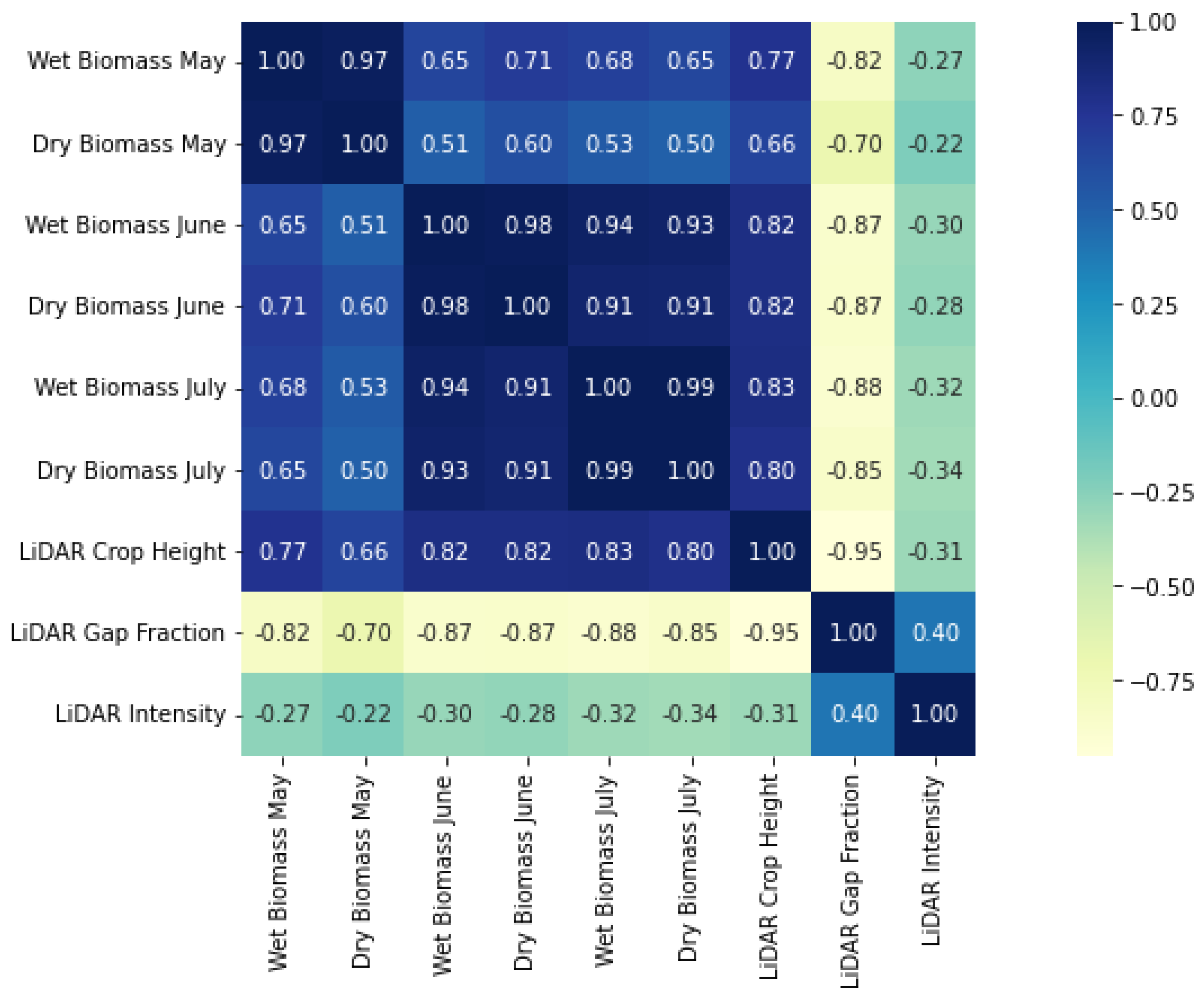
The three maps in Figure 3, Figure 4 and Figure 5 show a very similar spatial pattern, indicating a correlation between the LiDAR parameters. e.g., where significantly taller plants are, the gap fraction is significantly lower. Although the OLS results indicate that the LiDAR gap fraction provides highest potential to estimate AGB, the similarity of the spatial maps indicate common correlations. It is important to note that we do not encourage the utilization of the OLS equations to forward calculate wet and dry AGB from own LiDAR parameters due to limited number of samples to retrieve those equations, but we intended to provide an importance measure for individual LiDAR parameters. To clarify this further, a heat map of mutual correlation coefficients was generated and is displayed in Figure 7. Similar to Figure 6, the correlations of LiDAR parameters crop height and gap fraction to all AGB states and times is significant, whereas those of LiDAR intensity to these AGB states and times are not significant. Here, this anticipation is confirmed by correlation coefficients between LiDAR gap fraction and LiDAR crop height of −0.95. As discussed above, the relationship of LiDAR intensity to the other parameters is still complex and not easy to explain, resulting in correlation coefficients of 0.4 (gap fraction) and −0.31 (crop height), respectively.

Similarly, the VIF analysis shows that, with the coefficients of 11.10, 11.91, and 1.26 for crop height, gap fraction, and intensity, respectively, the first two parameters are highly collinear and are, in principle, exchangeable. However, the slightly higher absolute correlation coefficient between gap fraction and wet AGB (−0.82) than between crop height and wet AGB (0.77) is still informative.

An additional observation from Figure 7 is that the correlations between the LiDAR parameters crop height and gap fraction as well as the in situ samples obtained in May with the in situ samples in June and July are high. This indicates stable patterns in all observations over time. Especially, the wet biomass shows high temporal stability, so the LiDAR parameters crop height and gap fraction contain not only predictive power for the May AGB, but also for later stages in the phenological cycle. There is potential to estimate even at-harvest AGB. This opens up further applications of LiDAR observations in precision agriculture and agricultural management. The results indicate stable regions of crop growth favoring soil and topography conditions with higher crop height, lower gap fraction, and higher AGB. In contrast, in other regions, soil and topography conditions constrain crop growth with lower crop height, higher gap fraction, and lower AGB (see [40]). Therefore, the relationships between LiDAR parameters and AGB do not alter in general, but the predictive power may change with the phenological cycle. It seems that an observation in May, where the plants have already been widely developed, is a good point in time to predict AGB in the following months. The plants have already been exposed to the growth conditions, and a certain heterogeneity has been developed. More detailed time series analysis is needed to investigate the AGB predictive power throughout the phenological cycle and when observations are ideally taken.

The aim of this study was also to retrieve a highly spatial-detailed map of LiDAR parameters, so we defined the spatial resolution to be 15 cm. However, with generally 25–60 points per 15 cm grid cell, the uncertainties around adequately capturing the grid cell statistics (maximum height, minimum height, number of ground points, mean intensity) is quite high. Those uncertainties could be reduced by reducing the spatial resolution with larger grid cells and higher point numbers providing more robust LiDAR parameters.

5. Conclusions and Outlook

The results of this study indicate the potential of the LiDAR parameters crop height, gap fraction, and intensity to predict or invert aboveground biomass (AGB), with a slightly better performance for wet plant conditions. Especially, the gap fraction showed high correlations to AGB, as it is not just a piece of crop height information but denotes a simple representation of the full 3D plant structure. The LiDAR intensity needs further processing to provide valuable information about AGB. Here, a calibration could improve its information content. Additionally, application to crops other than cereals such as potato or sugar beet with broader leaves may provide different results.

The results of this study are limited to a single UAV flight campaign, but this already shows their potential to estimate future AGB states. A performance analysis of LiDAR parameters over the entire growing season to retrieve AGB is planned. Moreover, the calculation of parameters could be improved with finer representation of the full 3D plant structure. Similarly, the application of machine learning approaches could provide farmers with up-to-date information about their cultivates [41]. To move toward a small-scale cultivation structure, the LiDAR parameter retrieval methods at hand may be used for delineating cultivation zones with different growth conditions or even inverting toward soil characteristics such as soil texture, nutrient supply, or soil moisture.