
Hybrid LSTM-Based Fractional-Order Neural Network for Jeju Island’s Wind Farm Power Forecasting


Abstract
:1. Introduction
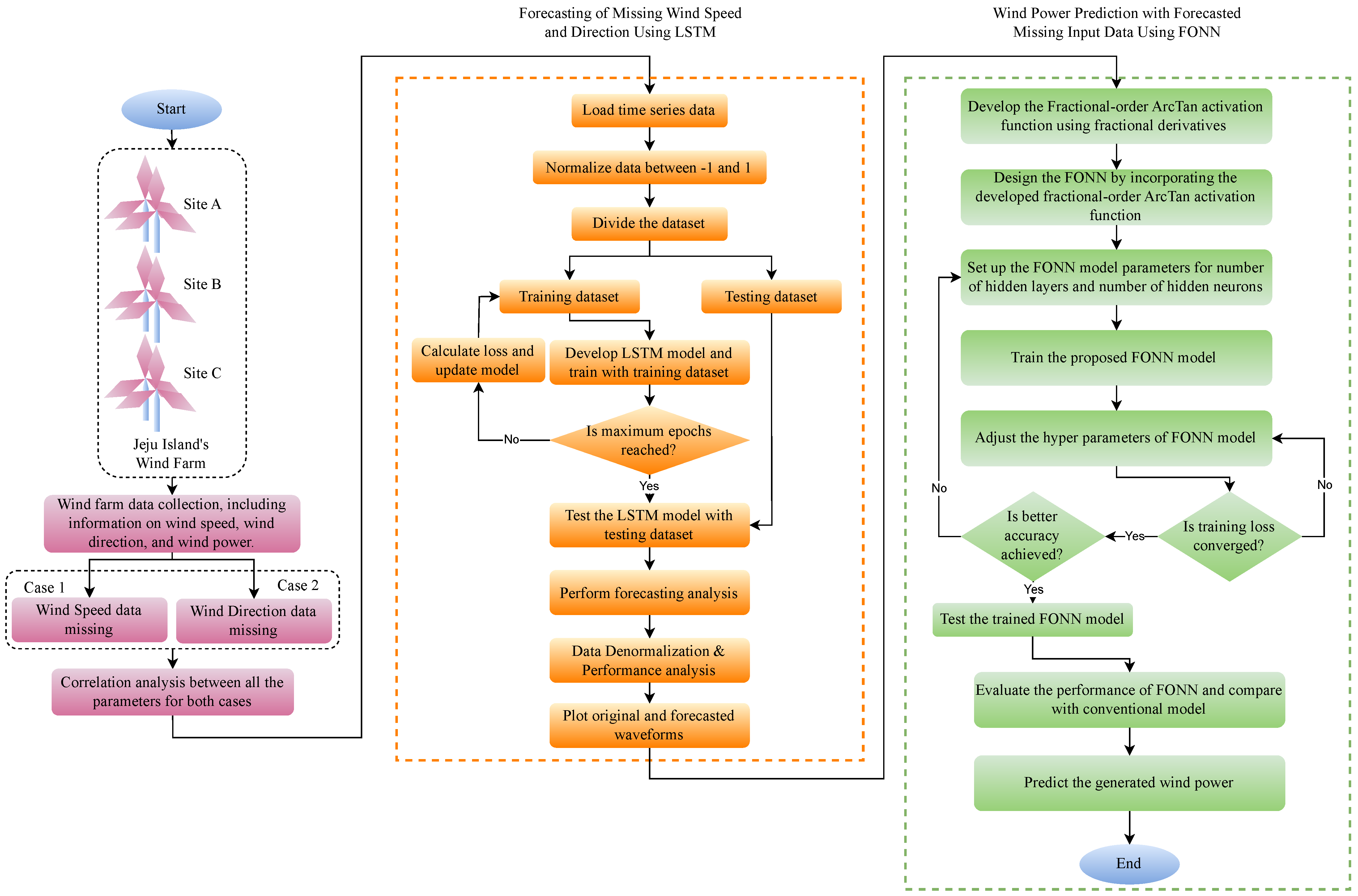
- The LSTM model is designed to predict missing input parameters, including wind speed and direction. Its performance is evaluated through root mean squared error (RMSE) assessment.
- The FONN model predicts wind power using the LSTM’s forecast data and evaluates performance with a coefficient of determination (R2) and mean squared error (MSE).
- The models developed were evaluated in two case studies involving missing data scenarios for specific parameters.
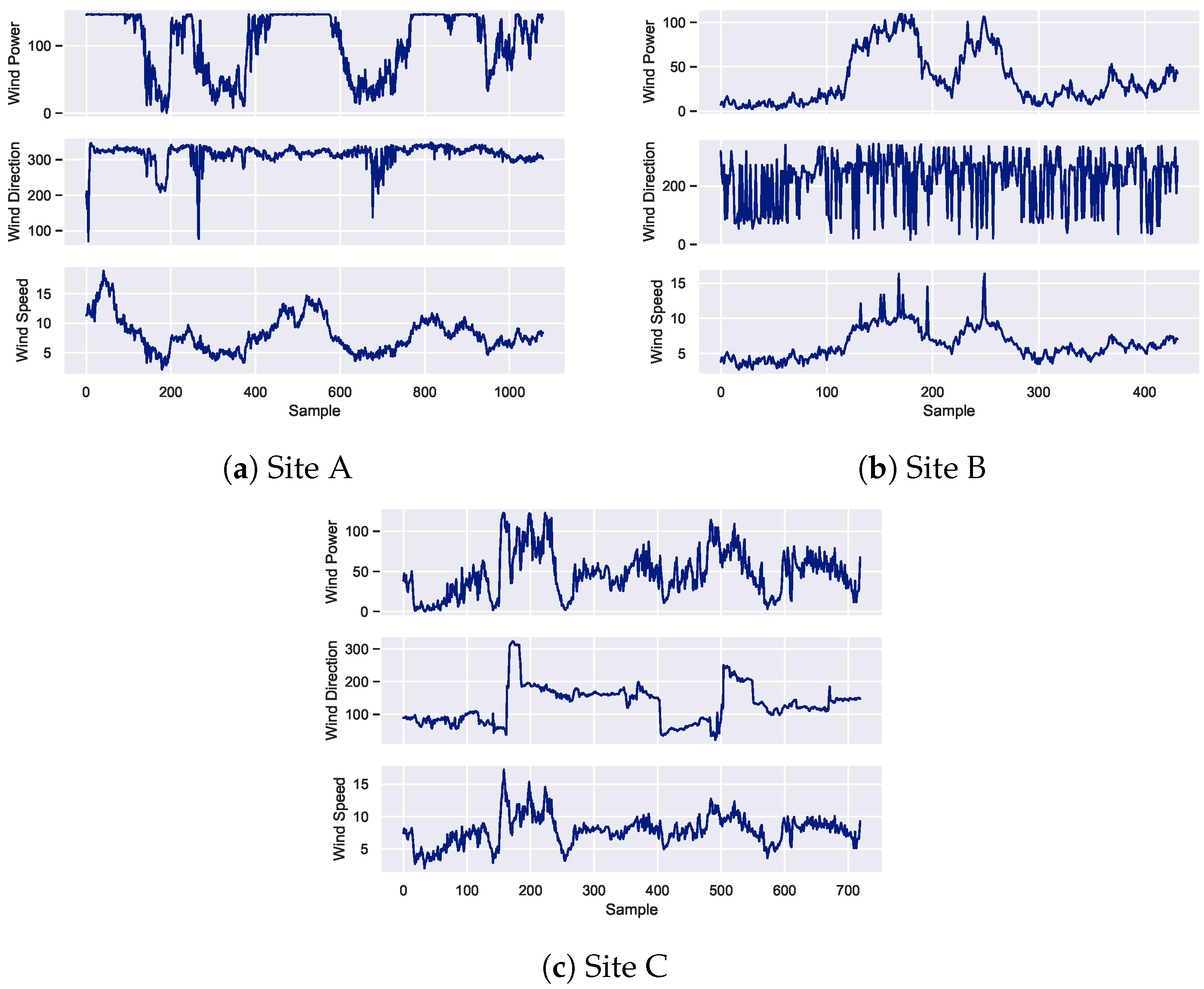
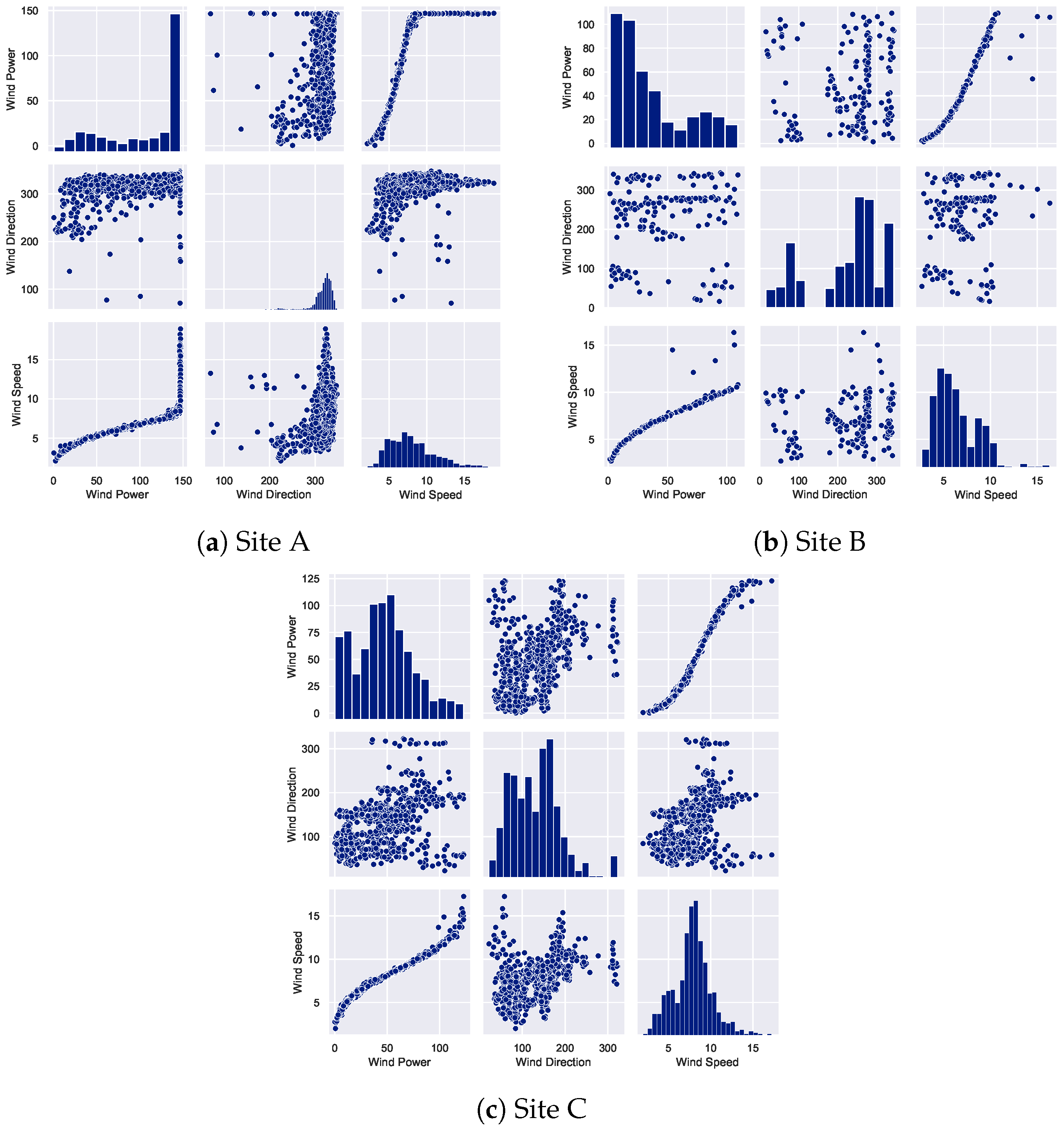
2. Dataset Description
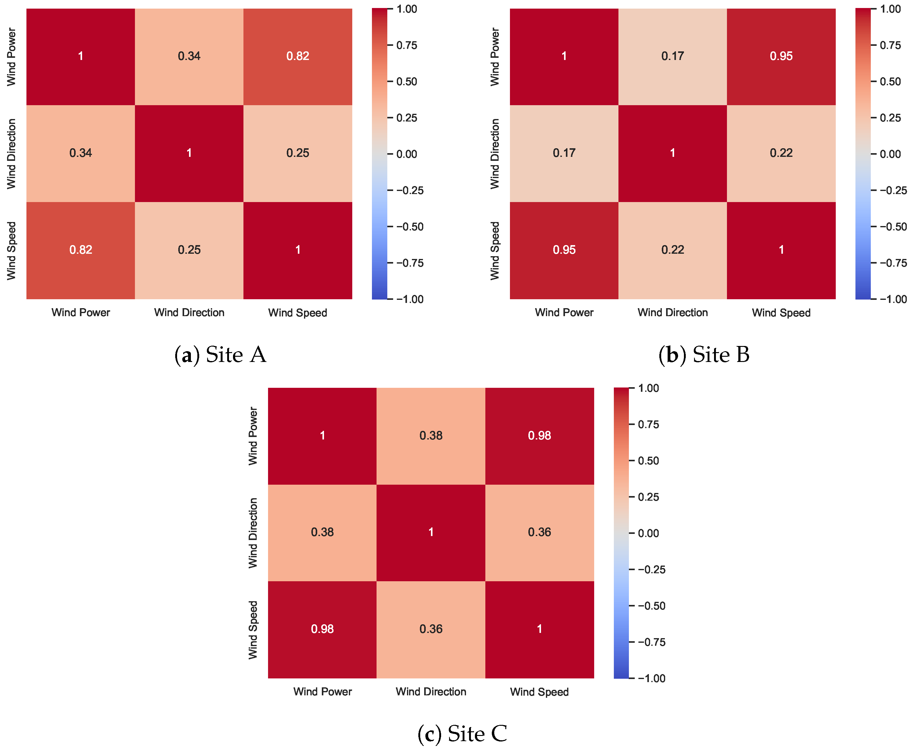
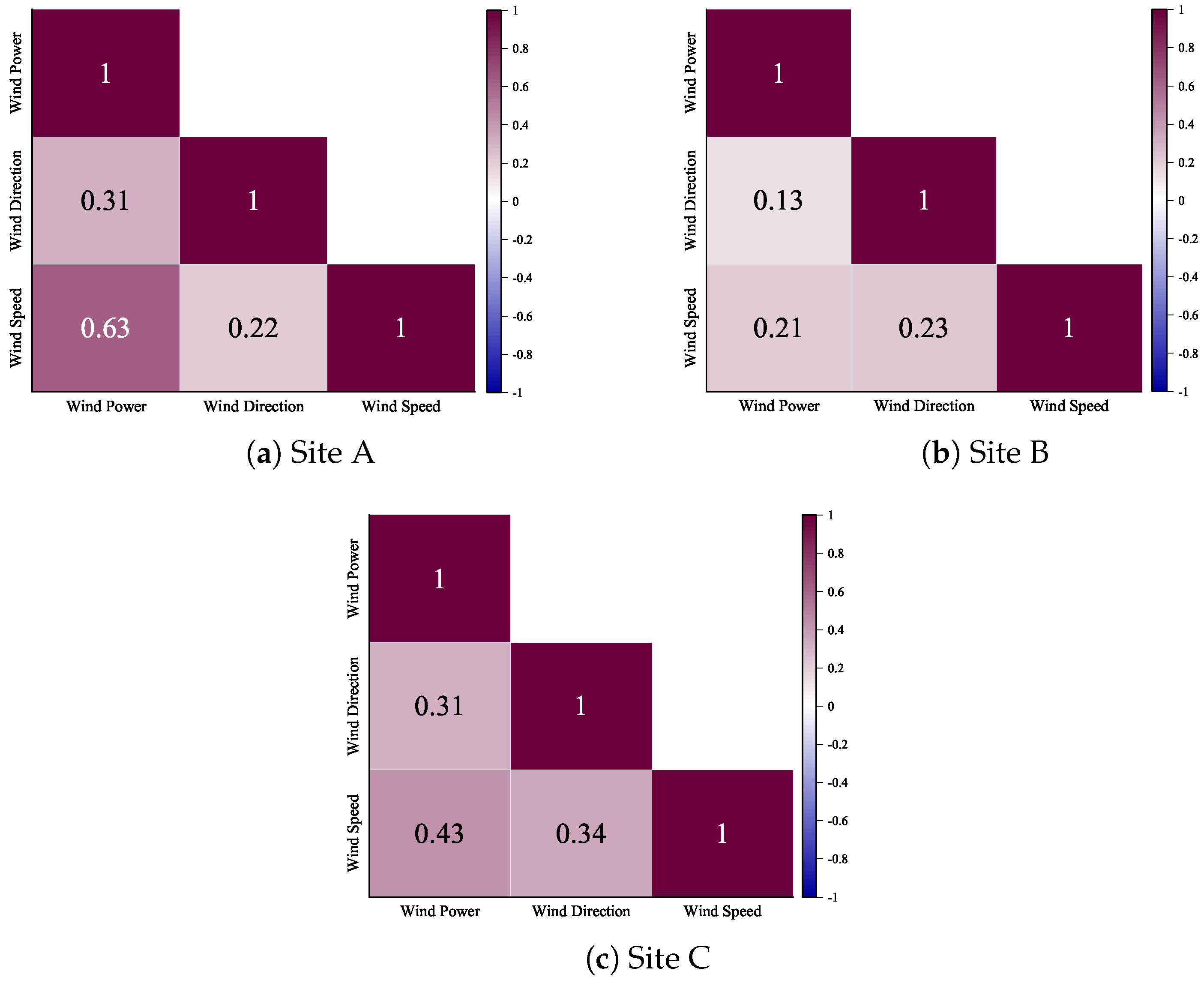
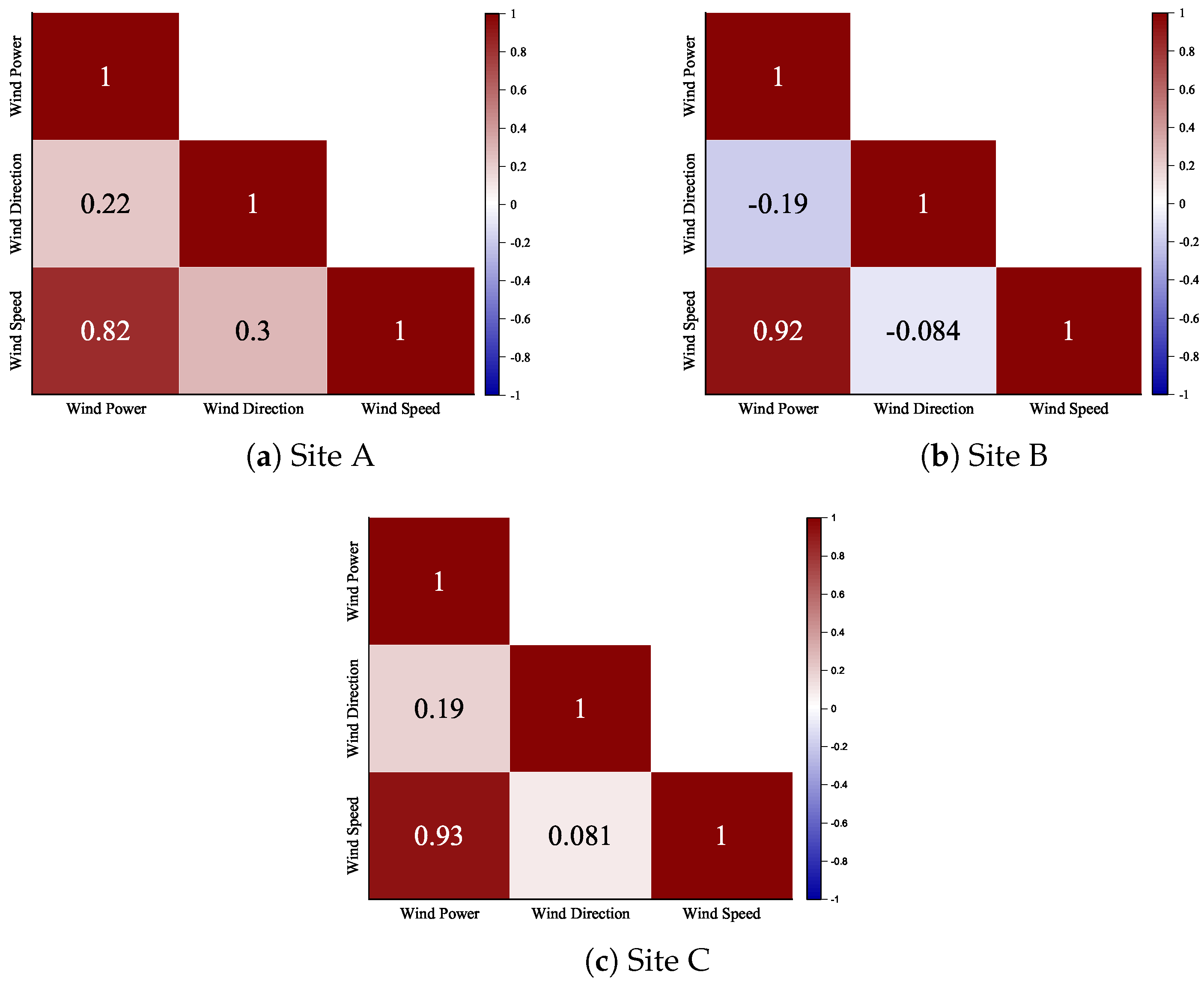
2.1. Correlation Analysis of Wind Speed Parameter with Missing Data
2.2. Correlation Analysis of Wind Direction Parameter with Missing Data
3. Proposed Methodology
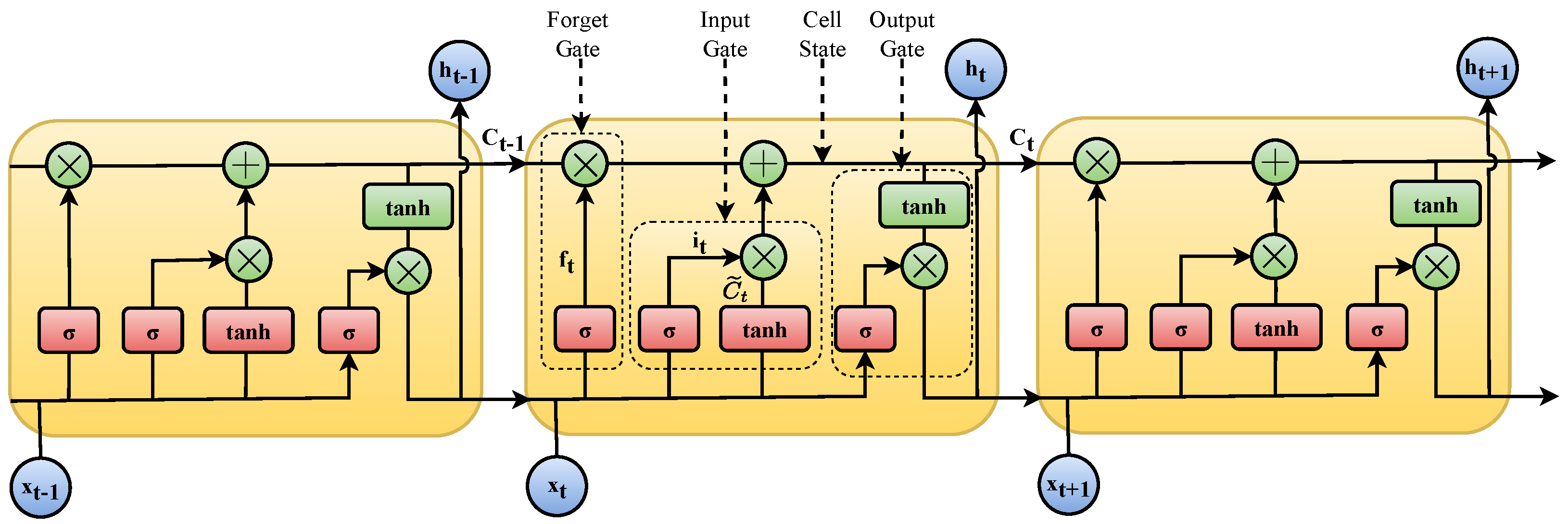
3.1. LSTM Model
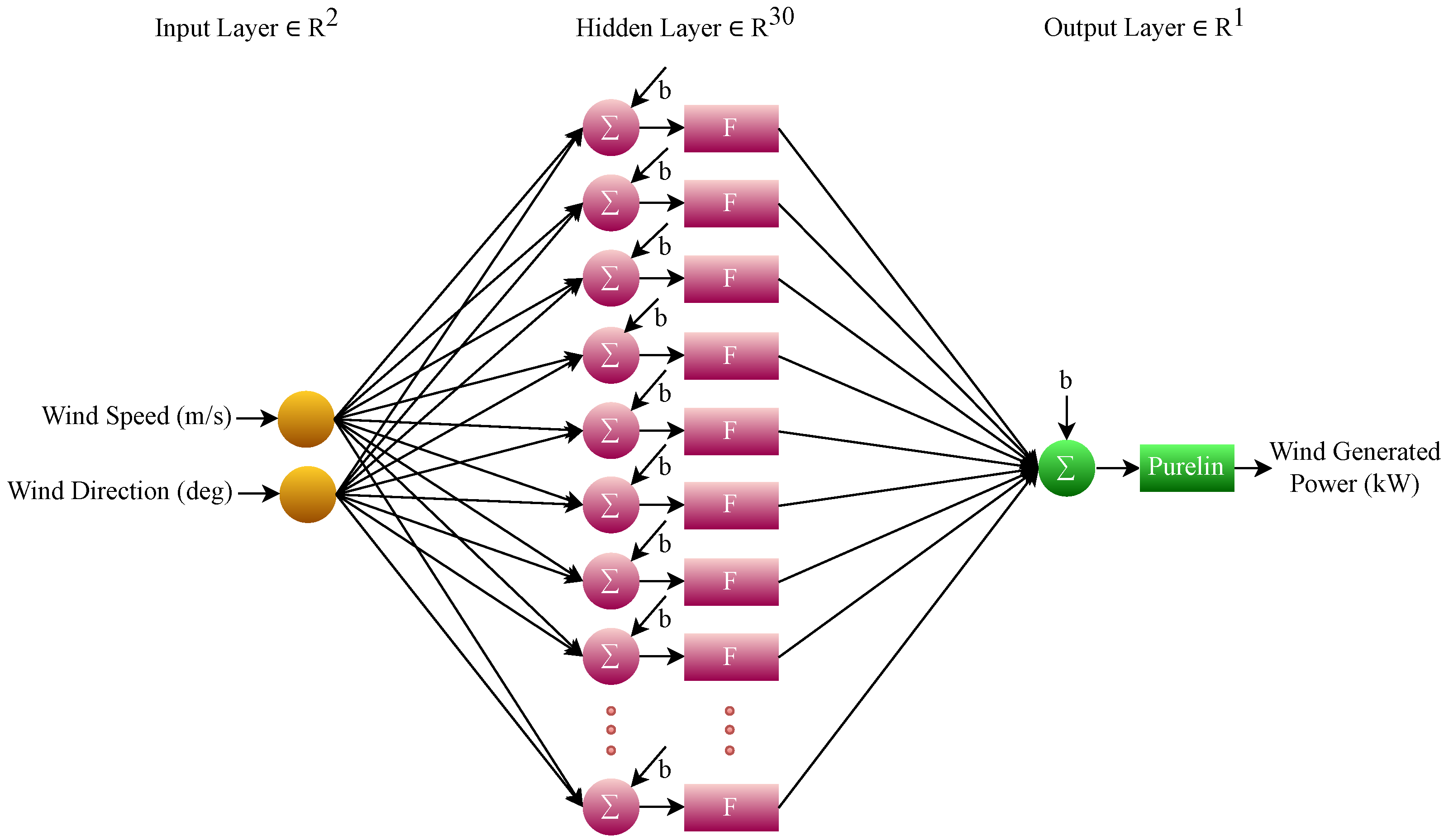
3.2. FONN Model
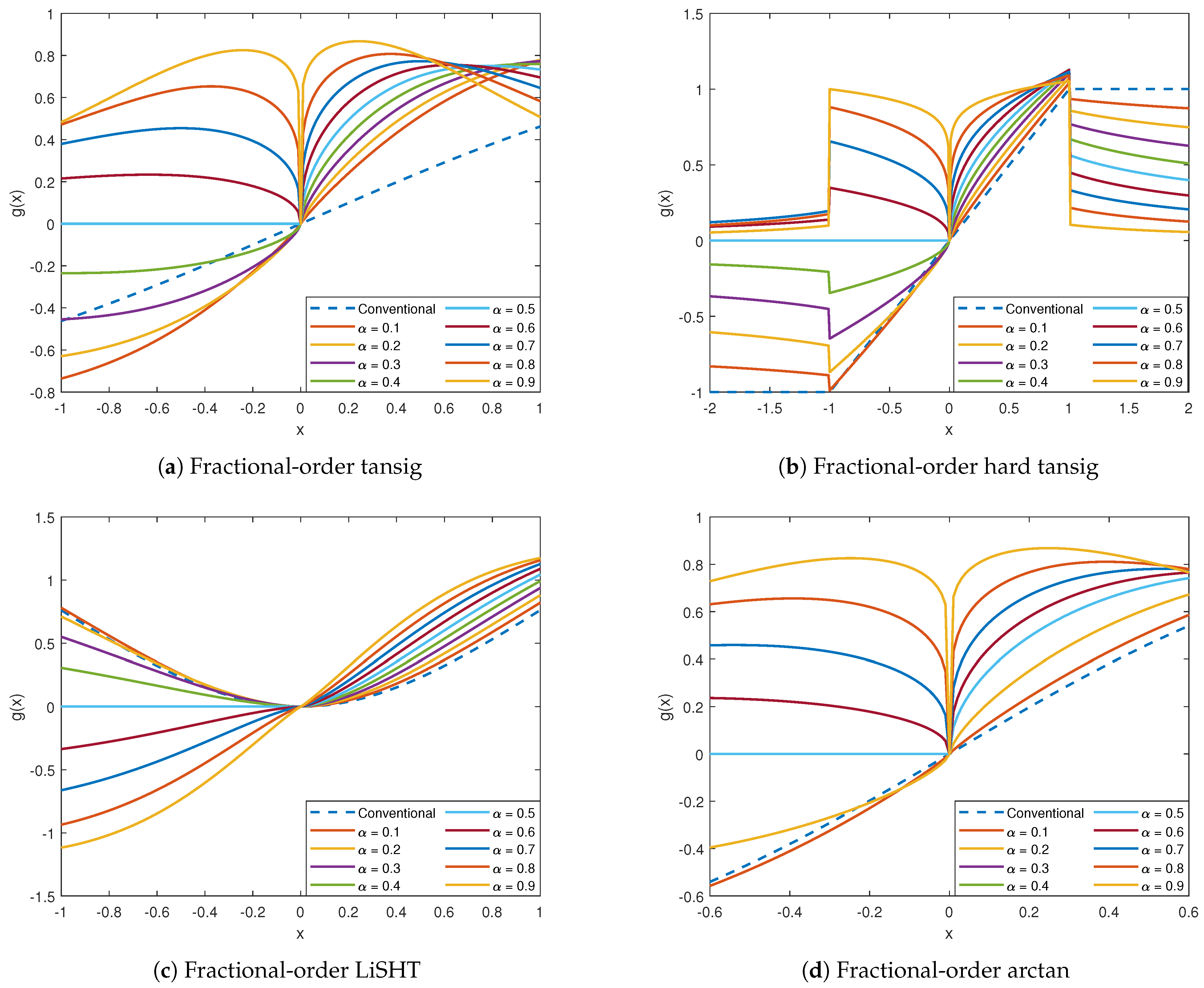
3.3. Fractional-Order Tangential Activation Functions
3.4. Performance Metrics
4. Results and Discussion
4.1. Performance of LSTM Model
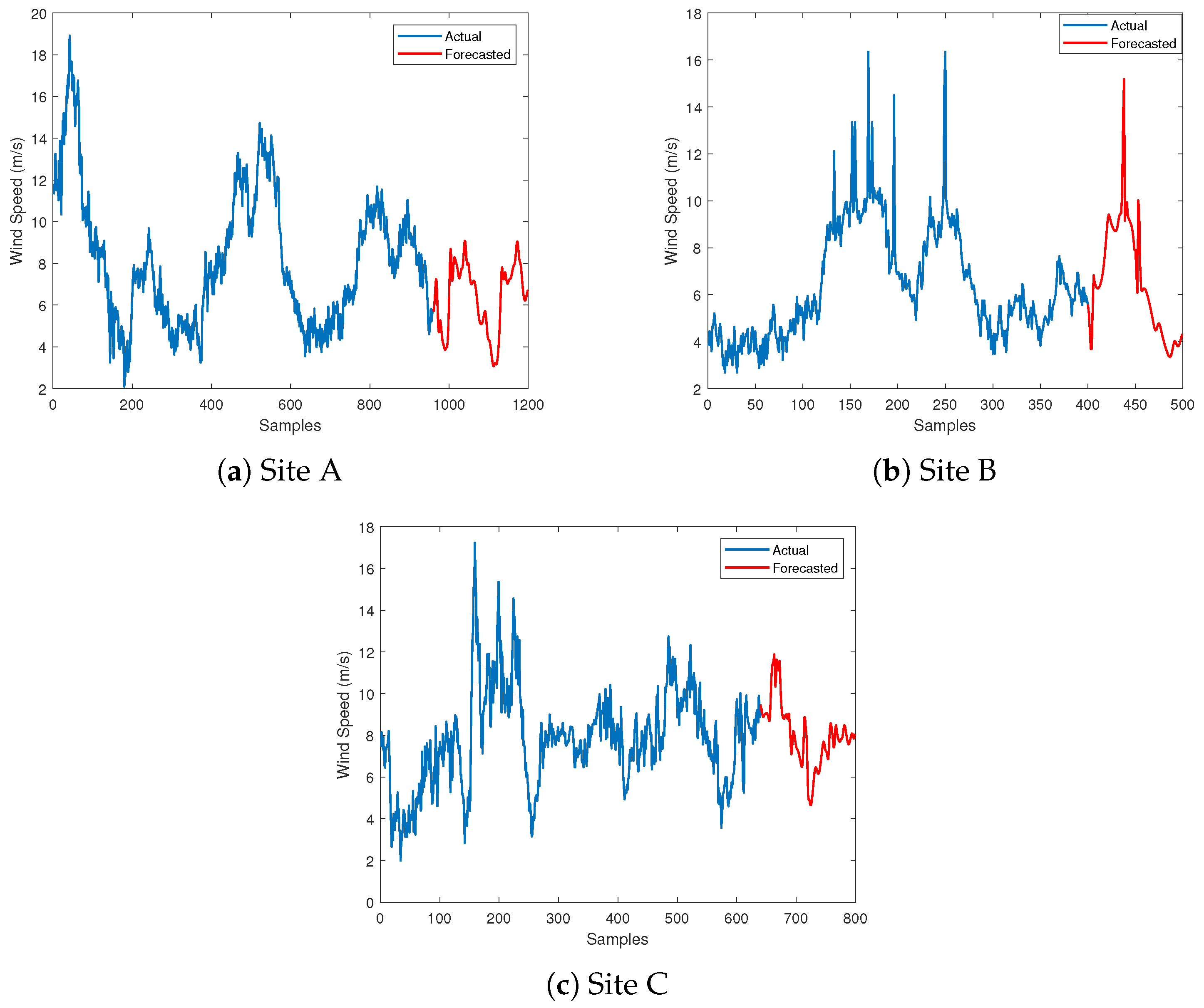
- The LSTM model exhibits the lowest RMSE values compared to the NAR and ARIMA models for forecasting missing wind speed data across all sites.
- At Site A, the LSTM model achieved the lowest RMSE value of 0.16, followed by NAR with an RMSE of 0.353 and ARIMA with an RMSE of 0.583.
- Similarly, the LSTM model at Site B outperformed the other models with an RMSE of 0.185, while the NAR and ARIMA models showed higher RMSE values of 0.297 and 0.458, respectively.
- Finally, at Site C, the LSTM model exhibited the lowest RMSE of 0.112, followed by ARIMA with an RMSE of 0.387 and NAR with the highest RMSE of 0.457.
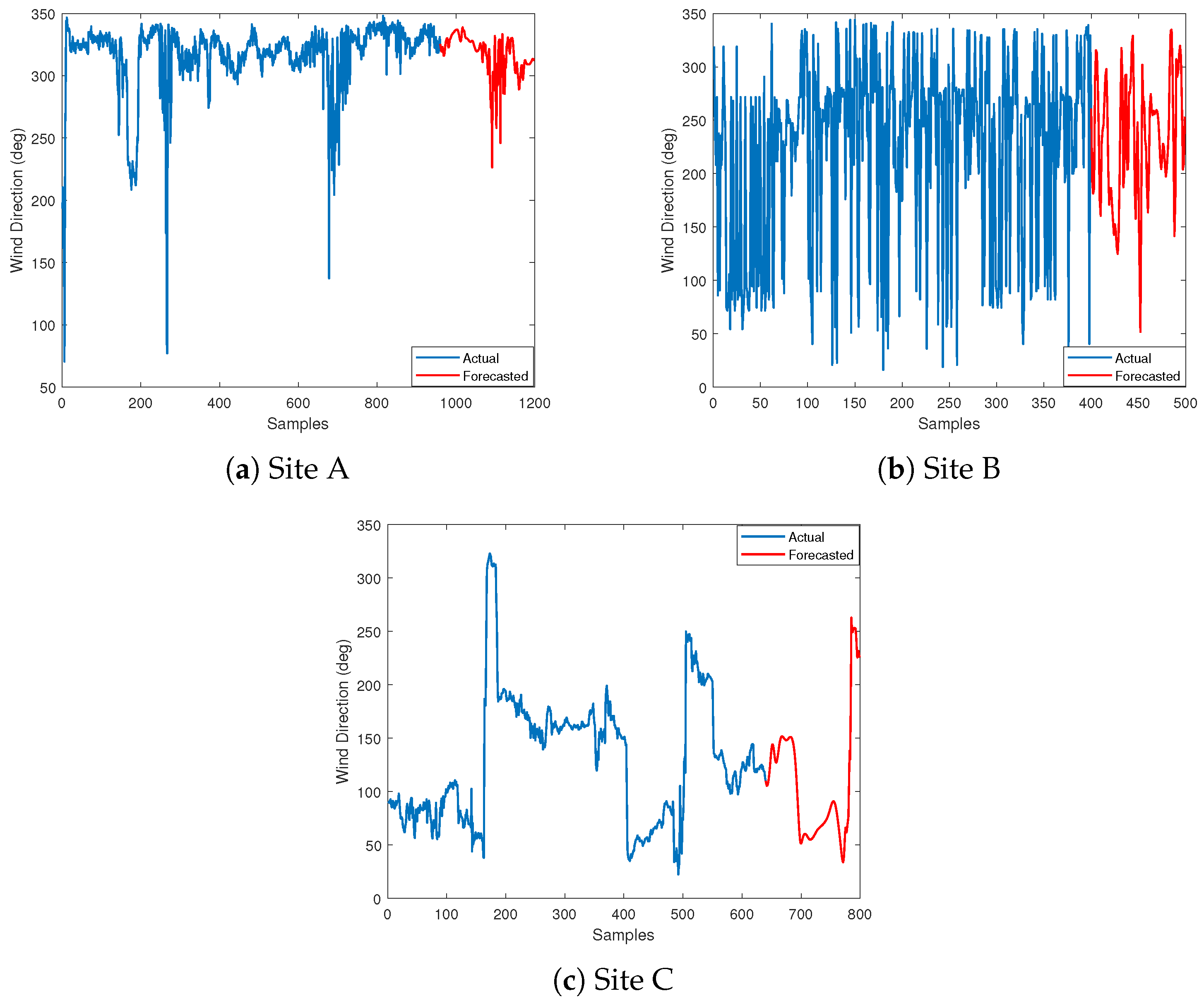
- The following analysis is related to missing wind direction data forecasting, where the performance of the models varies across different sites.
- At Site A, the LSTM model had the lowest RMSE of 0.18, followed by ARIMA with an RMSE of 0.386 and NAR with the highest RMSE of 0.442.
- Similarly, at Site B, the LSTM model performed best with an RMSE of 0.425, followed by NAR with an RMSE of 0.185, and ARIMA with the highest RMSE of 0.572.
- Finally, at Site C, the NAR model had the lowest RMSE of 0.395, followed by LSTM with an RMSE of 0.126, and ARIMA with the highest RMSE of 0.454.
4.2. Performance of FONN Model
4.2.1. Case Study 1
4.2.2. Case Study 2
5. Conclusions
Author Contributions
Funding
Data Availability Statement
Acknowledgments
Conflicts of Interest
References
- Kariniotakis, G.; Stavrakakis, G.; Nogaret, E. Wind power forecasting using advanced neural networks models. IEEE Trans. Energy Convers. 1996, 11, 762–767. [Google Scholar] [CrossRef]
- Han, Z.; Jing, Q.; Zhang, Y.; Bai, R.; Guo, K.; Zhang, Y. Review of wind power forecasting methods and new trends. Power Syst. Prot. Control 2019, 47, 178–187. [Google Scholar]
- Cui, Y.; Li, L.; Chen, D. Ultra-Short-Term Wind Power Load Forecast Based on Least Squares SVM. Electr. Autom. Pap. 2014, 5, 35–37. [Google Scholar]
- Zhang, Y.; Wang, P.; Ni, T.; Cheng, P.; Lei, S. Wind power prediction based on LS-SVM model with error correction. Adv. Electr. Comput. Eng. 2017, 17, 3–8. [Google Scholar] [CrossRef]
- Pinson, P.; Kariniotakis, G. Wind power forecasting using fuzzy neural networks enhanced with on-line prediction risk assessment. In Proceedings of the 2003 IEEE Bologna Power Tech Conference Proceedings, Bologna, Italy, 23–26 June 2003; Volume 2, p. 8. [Google Scholar]
- Shi, J.; Lee, W.J.; Liu, Y.; Yang, Y.; Wang, P. Short term wind power forecasting using Hilbert-Huang Transform and artificial neural network. In Proceedings of the 2011 4th International Conference on Electric Utility Deregulation and Restructuring and Power Technologies (DRPT), Weihai, China, 6–9 July 2011; pp. 162–167. [Google Scholar]
- Sideratos, G.; Hatziargyriou, N.D. Probabilistic wind power forecasting using radial basis function neural networks. IEEE Trans. Power Syst. 2012, 27, 1788–1796. [Google Scholar] [CrossRef]
- Hong, Y.Y.; Yu, T.H.; Liu, C.Y. Hour-ahead wind speed and power forecasting using empirical mode decomposition. Energies 2013, 6, 6137–6152. [Google Scholar] [CrossRef]
- Lotfi, E.; Khosravi, A.; Akbarzadeh-T, M.; Nahavandi, S. Wind power forecasting using emotional neural networks. In Proceedings of the 2014 IEEE International Conference on Systems, Man, and Cybernetics (SMC), San Diego, CA, USA, 5–8 October 2014; pp. 311–316. [Google Scholar]
- Chen, N.; Qian, Z.; Nabney, I.T.; Meng, X. Wind power forecasts using Gaussian processes and numerical weather prediction. IEEE Trans. Power Syst. 2013, 29, 656–665. [Google Scholar] [CrossRef]
- Çevik, H.H.; Acar, Y.E.; Çunkaş, M. Day ahead wind power forecasting using complex valued neural network. In Proceedings of the 2018 International Conference on Smart Energy Systems and Technologies (SEST), Seville, Spain, 10–12 September 2018; pp. 1–6. [Google Scholar]
- Naik, J.; Dash, S.; Dash, P.K.; Bisoi, R. Short term wind power forecasting using hybrid variational mode decomposition and multi-kernel regularized pseudo inverse neural network. Renew. Energy 2018, 118, 180–212. [Google Scholar] [CrossRef]
- Higashiyama, K.; Fujimoto, Y.; Hayashi, Y. Feature extraction of NWP data for wind power forecasting using 3D-convolutional neural networks. Energy Procedia 2018, 155, 350–358. [Google Scholar] [CrossRef]
- Abesamis, K.; Ang, P.; Bisquera, F.I.; Catabay, G.; Tindogan, P.; Ostia, C.; Pacis, M. Short-Term Wind Power Forecasting Using Structured Neural Network. In Proceedings of the 2019 IEEE 11th International Conference on Humanoid, Nanotechnology, Information Technology, Communication and Control, Environment, and Management (HNICEM), Laoag, Philippines, 29 November–1 December 2019; pp. 1–4. [Google Scholar]
- Ansari, S.; Sampath Vinayak Kumar, T.G.; Dhillon, J. Wind Power Forecasting using Artificial Neural Network. In Proceedings of the 2021 4th International Conference on Recent Developments in Control, Automation & Power Engineering (RDCAPE), Noida, India, 7–8 October 2021; pp. 35–37. [Google Scholar] [CrossRef]
- Khelil, K.; Berrezzek, F.; Bouadjila, T. DWT-based Wind Speed Forecasting Using Artificial Neural Networks in the region of Annaba. In Proceedings of the 2020 1st International Conference on Communications, Control Systems and Signal Processing (CCSSP), El Oued, Algeria, 16–17 May 2020; pp. 508–512. [Google Scholar]
- Jørgensen, K.L.; Shaker, H.R. Wind power forecasting using machine learning: State of the art, trends and challenges. In Proceedings of the 2020 IEEE 8th International Conference on Smart Energy Grid Engineering (SEGE), Oshawa, ON, Canada, 12–14 August 2020; pp. 44–50. [Google Scholar]
- Lipu, M.H.; Miah, M.S.; Hannan, M.; Hussain, A.; Sarker, M.R.; Ayob, A.; Saad, M.H.M.; Mahmud, M.S. Artificial intelligence based hybrid forecasting approaches for wind power generation: Progress, challenges and prospects. IEEE Access 2021, 9, 102460–102489. [Google Scholar] [CrossRef]
- Peiris, A.T.; Jayasinghe, J.; Rathnayake, U. Forecasting wind power generation using artificial neural network:“Pawan Danawi”—A case study from Sri Lanka. J. Electr. Comput. Eng. 2021, 2021, 5577547. [Google Scholar] [CrossRef]
- He, Y.; Li, H. Probability density forecasting of wind power using quantile regression neural network and kernel density estimation. Energy Convers. Manag. 2018, 164, 374–384. [Google Scholar] [CrossRef]
- Wu, Y.X.; Wu, Q.B.; Zhu, J.Q. Data-driven wind speed forecasting using deep feature extraction and LSTM. IET Renew. Power Gener. 2019, 13, 2062–2069. [Google Scholar] [CrossRef]
- Ramadevi, B.; Bingi, K. Chaotic time series forecasting approaches using machine learning techniques: A review. Symmetry 2022, 14, 955. [Google Scholar] [CrossRef]
- Vaswani, A.; Shazeer, N.; Parmar, N.; Uszkoreit, J.; Jones, L.; Gomez, A.N.; Kaiser, Ł.; Polosukhin, I. Attention is all you need. arXiv 2017, arXiv:1706.03762. [Google Scholar] [CrossRef]
- Zhu, Q.; Li, H.; Wang, Z.; Chen, J.; Wang, B. Ultra-short-term prediction of wind farm power generation based on long-and short-term memory networks. Power Grid Technol. 2017, 41, 3797–3802. [Google Scholar]
- Wang, S.; Li, B.; Li, G.; Yao, B.; Wu, J. Short-term wind power prediction based on multidimensional data cleaning and feature reconfiguration. Appl. Energy 2021, 292, 116851. [Google Scholar] [CrossRef]
- Khochare, J.; Rathod, J.; Joshi, C.; Laveti, R.N. A short-term wind forecasting framework using ensemble learning for indian weather stations. In Proceedings of the 2020 IEEE International Conference for Innovation in Technology (INOCON), Bangluru, India, 6–8 November 2020; pp. 1–7. [Google Scholar]
- Kumar, D.; Abhinav, R.; Pindoriya, N. An ensemble model for short-term wind power forecasting using deep learning and gradient boosting algorithms. In Proceedings of the 2020 21st National Power Systems Conference (NPSC), Gandhinagar, India, 17–19 December 2020; pp. 1–6. [Google Scholar]
- Zhou, M.; Wang, B.; Guo, S.; Watada, J. Multi-objective prediction intervals for wind power forecast based on deep neural networks. Inf. Sci. 2021, 550, 207–220. [Google Scholar] [CrossRef]
- Zhang, Y.; Li, Y.; Zhang, G. Short-term wind power forecasting approach based on Seq2Seq model using NWP data. Energy 2020, 213, 118371. [Google Scholar] [CrossRef]
- Kisvari, A.; Lin, Z.; Liu, X. Wind power forecasting—A data-driven method along with gated recurrent neural network. Renew. Energy 2021, 163, 1895–1909. [Google Scholar] [CrossRef]
- Lin, W.H.; Wang, P.; Chao, K.M.; Lin, H.C.; Yang, Z.Y.; Lai, Y.H. Wind power forecasting with deep learning networks: Time-series forecasting. Appl. Sci. 2021, 11, 10335. [Google Scholar] [CrossRef]
- Cali, U.; Sharma, V. Short-term wind power forecasting using long-short term memory based recurrent neural network model and variable selection. Int. J. Smart Grid Clean Energy 2019, 8, 103–110. [Google Scholar] [CrossRef]
- Zhang, K.; Jin, H.; Jin, H.; Wang, B.; Yu, W. Gated Recurrent Unit Neural Networks for Wind Power Forecasting based on Surrogate-Assisted Evolutionary Neural Architecture Search. In Proceedings of the 2023 IEEE 12th Data Driven Control and Learning Systems Conference (DDCLS), Xiangtan, China, 12–14 May 2023; pp. 1774–1779. [Google Scholar]
- Arora, P.; Jalali, S.M.J.; Ahmadian, S.; Panigrahi, B.; Suganthan, P.; Khosravi, A. Probabilistic Wind Power Forecasting Using Optimized Deep Auto-Regressive Recurrent Neural Networks. IEEE Trans. Ind. Inform. 2022, 19, 2814–2825. [Google Scholar] [CrossRef]
- Miele, E.S.; Ludwig, N.; Corsini, A. Multi-Horizon Wind Power Forecasting Using Multi-Modal Spatio-Temporal Neural Networks. Energies 2023, 16, 3522. [Google Scholar] [CrossRef]
- Wu, N.; Green, B.; Ben, X.; O’Banion, S. Deep transformer models for time series forecasting: The influenza prevalence case. arXiv 2020, arXiv:2001.08317. [Google Scholar]
- Han, K.; Xiao, A.; Wu, E.; Guo, J.; Xu, C.; Wang, Y. Transformer in transformer. Adv. Neural Inf. Process. Syst. 2021, 34, 15908–15919. [Google Scholar]
- Ren, J.; Yu, Z.; Gao, G.; Yu, G.; Yu, J. A CNN-LSTM-LightGBM based short-term wind power prediction method based on attention mechanism. Energy Rep. 2022, 8, 437–443. [Google Scholar] [CrossRef]
- Zhou, X.; Liu, C.; Luo, Y.; Wu, B.; Dong, N.; Xiao, T.; Zhu, H. Wind power forecast based on variational mode decomposition and long short term memory attention network. Energy Rep. 2022, 8, 922–931. [Google Scholar] [CrossRef]
- Wang, L.; He, Y.; Li, L.; Liu, X.; Zhao, Y. A novel approach to ultra-short-term multi-step wind power predictions based on encoder–decoder architecture in natural language processing. J. Clean. Prod. 2022, 354, 131723. [Google Scholar] [CrossRef]
- Wei, H.; Wang, W.s.; Kao, X.x. A novel approach to ultra-short-term wind power prediction based on feature engineering and informer. Energy Rep. 2023, 9, 1236–1250. [Google Scholar] [CrossRef]
- Ramadevi, B.; Kasi, V.R.; Bingi, K. Fractional ordering of activation functions for neural networks: A case study on Texas wind turbine. Eng. Appl. Artif. Intell. 2024, 127, 107308. [Google Scholar] [CrossRef]
- Esquivel, J.Z.; Vargas, J.A.C.; Lopez-Meyer, P. Fractional adaptation of activation functions in neural networks. In Proceedings of the 2020 25th International Conference on Pattern Recognition (ICPR), Milan, Italy, 10–15 January 2021; pp. 7544–7550. [Google Scholar]
- Son, N.; Yang, S.; Na, J. Hybrid forecasting model for short-term wind power prediction using modified long short-term memory. Energies 2019, 12, 3901. [Google Scholar] [CrossRef]
- Dubey, S.R.; Singh, S.K.; Chaudhuri, B.B. A comprehensive survey and performance analysis of activation functions in deep learning. arXiv 2021, arXiv:2109.14545. [Google Scholar]
- Ding, B.; Qian, H.; Zhou, J. Activation functions and their characteristics in deep neural networks. In Proceedings of the 2018 Chinese Control and Decision Conference (CCDC), Shenyang, China, 9–11 June 2018; pp. 1836–1841. [Google Scholar]
- Nwankpa, C.; Ijomah, W.; Gachagan, A.; Marshall, S. Activation functions: Comparison of trends in practice and research for deep learning. arXiv 2018, arXiv:1811.03378. [Google Scholar]
- Lederer, J. Activation functions in artificial neural networks: A systematic overview. arXiv 2021, arXiv:2101.09957. [Google Scholar]
- Job, M.S.; Bhateja, P.H.; Gupta, M.; Bingi, K.; Prusty, B.R. Fractional Rectified Linear Unit Activation Function and Its Variants. Math. Probl. Eng. 2022, 2022, 1860779. [Google Scholar] [CrossRef]
- Sharma, S.; Sharma, S.; Athaiya, A. Activation functions in neural networks. Towards Data Sci. 2017, 6, 310–316. [Google Scholar] [CrossRef]
- Adhikari, R.; Agrawal, R.K. An introductory study on time series modeling and forecasting. arXiv 2013, arXiv:1302.6613. [Google Scholar]
- Bingi, K.; Prusty, B.R.; Kumra, A.; Chawla, A. Torque and temperature prediction for permanent magnet synchronous motor using neural networks. In Proceedings of the 2020 3rd International Conference on Energy, Power and Environment: Towards Clean Energy Technologies, Shillong, India, 5–7 March 2021; pp. 1–6. [Google Scholar]
- Ramadevi, B.; Bingi, K. Time Series Forecasting Model for Sunspot Number. In Proceedings of the 2022 International Conference on Intelligent Controller and Computing for Smart Power (ICICCSP), Hyderabad, India, 21–23 July 2022; pp. 1–6. [Google Scholar] [CrossRef]
- Siami-Namini, S.; Tavakoli, N.; Siami Namin, A. A Comparison of ARIMA and LSTM in Forecasting Time Series. In Proceedings of the 2018 17th IEEE International Conference on Machine Learning and Applications (ICMLA), Orlando, FL, USA, 17–20 December 2018; pp. 1394–1401. [Google Scholar] [CrossRef]


| Data Aspect | Site A | Site B | Site C |
|---|---|---|---|
| Data Collection Period | 11 January 2014–25 January 2014 | 11 January 2014–20 January 2014 | 11 January 2014–25 January 2014 |
| Collection Time Interval | 10 min | 10 min | 10 min |
| Wind Turbine Specifications | |||
| Model | U88 | U50 | U50 |
| Output | 2000 kW | 750 kW | 750 kW |
| Wind Speed | Up to 12 m/s | Up to 12.5 m/s | Up to 12.5 m/s |
| Rotor Speed Range | 6–17.5 rpm | 9–28 rpm | 9–28 rpm |
| Voltage and Frequency | 690 V/60 Hz | 690 V/60 Hz | 690 V/60 Hz |
| Rotor Diameter | 88 m | 50 m | 50 m |
| Hub Height | 80 m | 50 m | 50 m |
| Power Control | Pitch Regulation | Pitch Regulation | Pitch Regulation |
| Model | Site | Wind Speed (m/s) | Wind Direction (deg) |
|---|---|---|---|
| RMSE | RMSE | ||
| LSTM | Site A | 0.18 | 0.16 |
| Site B | 0.425 | 0.185 | |
| Site C | 0.112 | 0.126 | |
| NAR | Site A | 0.353 | 0.442 |
| Site B | 0.297 | 0.185 | |
| Site C | 0.457 | 0.395 | |
| ARIMA | Site A | 0.583 | 0.386 |
| Site B | 0.458 | 0.572 | |
| Site C | 0.387 | 0.454 |
| Site | Conventional Function | Training | Testing | Fractional Function | Training | Testing | ||||
|---|---|---|---|---|---|---|---|---|---|---|
| R2 | MSE | R2 | MSE | R2 | MSE | R2 | MSE | |||
| Site A | Tansig | 0.8578 | 0.0753 | 0.8642 | 0.0764 | Tansig | 0.8739 | 0.0628 | 0.8864 | 0.0612 |
| Hard tansig | 0.8954 | 0.0521 | 0.9075 | 0.0516 | Hard tansig | 0.9263 | 0.0424 | 0.9369 | 0.0397 | |
| LiSHT | 0.8749 | 0.0683 | 0.8873 | 0.0621 | LiSHT | 0.9025 | 0.0612 | 0.9173 | 0.0598 | |
| Arctan | 0.9727 | 0.0227 | 0.9733 | 0.0207 | Arctan | 0.9749 | 0.0205 | 0.9831 | 0.0142 | |
| Site B | Tansig | 0.9328 | 0.0662 | 0.9436 | 0.0652 | Tansig | 0.9428 | 0.0534 | 0.9497 | 0.0529 |
| Hard tansig | 0.9489 | 0.0583 | 0.9517 | 0.0578 | Hard tansig | 0.9543 | 0.0464 | 0.9609 | 0.0432 | |
| LiSHT | 0.9532 | 0.0428 | 0.9584 | 0.0414 | LiSHT | 0.9572 | 0.0399 | 0.9621 | 0.0386 | |
| Arctan | 0.9901 | 0.0063 | 0.9948 | 0.0035 | Arctan | 0.9929 | 0.0046 | 0.9952 | 0.0032 | |
| Site C | Tansig | 0.8216 | 0.0853 | 0.8362 | 0.0817 | Tansig | 0.8931 | 0.0742 | 0.9026 | 0.0629 |
| Hard tansig | 0.8453 | 0.0732 | 0.8564 | 0.0695 | Hard tansig | 0.9035 | 0.0598 | 0.9163 | 0.0586 | |
| LiSHT | 0.8762 | 0.0789 | 0.8758 | 0.0778 | LiSHT | 0.8864 | 0.0752 | 0.8973 | 0.0745 | |
| Arctan | 0.9469 | 0.0158 | 0.9529 | 0.0134 | Arctan | 0.9573 | 0.0123 | 0.9635 | 0.0115 | |
| Site | Conventional Function | Training | Testing | Fractional Function | Training | Testing | ||||
|---|---|---|---|---|---|---|---|---|---|---|
| R2 | MSE | R2 | MSE | R2 | MSE | R2 | MSE | |||
| Site A | Tansig | 0.8973 | 0.0621 | 0.9043 | 0.0594 | Tansig | 0.9264 | 0.0519 | 0.9329 | 0.0497 |
| Hard tansig | 0.9264 | 0.0372 | 0.9378 | 0.0346 | Hard tansig | 0.9726 | 0.0218 | 0.9832 | 0.0169 | |
| LiSHT | 0.9163 | 0.0583 | 0.9289 | 0.0542 | LiSHT | 0.9517 | 0.0487 | 0.9619 | 0.0453 | |
| Arctan | 0.9898 | 0.0081 | 0.9931 | 0.0059 | Arctan | 0.9899 | 0.0081 | 0.9946 | 0.0048 | |
| Site B | Tansig | 0.8245 | 0.0982 | 0.8463 | 0.0968 | Tansig | 0.8562 | 0.0841 | 0.8678 | 0.0832 |
| Hard tansig | 0.8674 | 0.0721 | 0.8689 | 0.0708 | Hard tansig | 0.8864 | 0.0682 | 0.8949 | 0.0617 | |
| LiSHT | 0.8462 | 0.0819 | 0.8573 | 0.0798 | LiSHT | 0.8693 | 0.0739 | 0.8715 | 0.0716 | |
| Arctan | 0.9826 | 0.0129 | 0.9875 | 0.0094 | Arctan | 0.9835 | 0.0124 | 0.9867 | 0.0094 | |
| Site C | Tansig | 0.9041 | 0.0528 | 0.9146 | 0.0512 | Tansig | 0.9317 | 0.0425 | 0.9462 | 0.0419 |
| Hard tansig | 0.9089 | 0.0481 | 0.9163 | 0.0479 | Hard tansig | 0.9273 | 0.0341 | 0.9526 | 0.0252 | |
| LiSHT | 0.8932 | 0.0514 | 0.9023 | 0.0506 | LiSHT | 0.9172 | 0.0459 | 0.9251 | 0.0445 | |
| Arctan | 0.9793 | 0.0085 | 0.9866 | 0.0054 | Arctan | 0.9816 | 0.0076 | 0.9865 | 0.0052 | |
Disclaimer/Publisher’s Note: The statements, opinions and data contained in all publications are solely those of the individual author(s) and contributor(s) and not of MDPI and/or the editor(s). MDPI and/or the editor(s) disclaim responsibility for any injury to people or property resulting from any ideas, methods, instructions or products referred to in the content. |
© 2024 by the authors. Licensee MDPI, Basel, Switzerland. This article is an open access article distributed under the terms and conditions of the Creative Commons Attribution (CC BY) license (https://creativecommons.org/licenses/by/4.0/).
Share and Cite
Ramadevi, B.; Kasi, V.R.; Bingi, K. Hybrid LSTM-Based Fractional-Order Neural Network for Jeju Island’s Wind Farm Power Forecasting. Fractal Fract. 2024, 8, 149. https://doi.org/10.3390/fractalfract8030149
Ramadevi B, Kasi VR, Bingi K. Hybrid LSTM-Based Fractional-Order Neural Network for Jeju Island’s Wind Farm Power Forecasting. Fractal and Fractional. 2024; 8(3):149. https://doi.org/10.3390/fractalfract8030149
Chicago/Turabian StyleRamadevi, Bhukya, Venkata Ramana Kasi, and Kishore Bingi. 2024. "Hybrid LSTM-Based Fractional-Order Neural Network for Jeju Island’s Wind Farm Power Forecasting" Fractal and Fractional 8, no. 3: 149. https://doi.org/10.3390/fractalfract8030149