
A Class of Fifth-Order Chebyshev–Halley-Type Iterative Methods and Its Stability Analysis

Abstract
:1. Introduction
2. Convergence of the New Family
3. Complex Dynamics Behavior
3.1. Rational Operator
3.2. Analysis and Stability of Fixed Points
- •
- If , the polynomials and have common factors , in which case the operator has seven strange fixed points .
- •
- If , the operator has six strange fixed points .
- •
- If α satisfies , the operator has nine strange fixed points: and eight roots of the polynomial .
- •
- Suppose that are some values of and ; by concatenating the two polynomial equations, we can eliminate the parameter , at which time we obtain , from which we know that can be a common factor of and . So, if we put into and , we obtain . Now operator has seven strange fixed points.
- •
- The remaining cases are obviously as shown in the above theorem.
- •
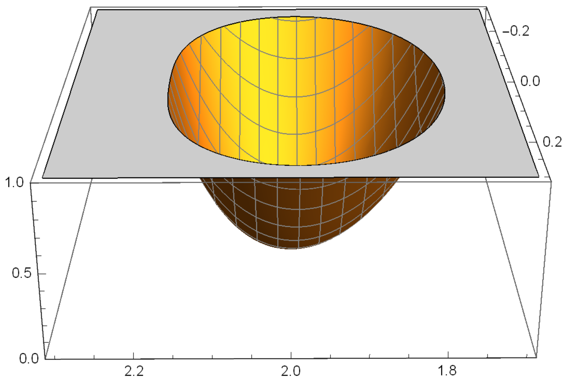
- , taking parameter values in the region of the complex plane is an attractor. And z = 1 is a superattractive fixed point for ; is a hyperbolic fixed point for and .
- •
- are repulsive, with independence of the value of parameter α.
- •
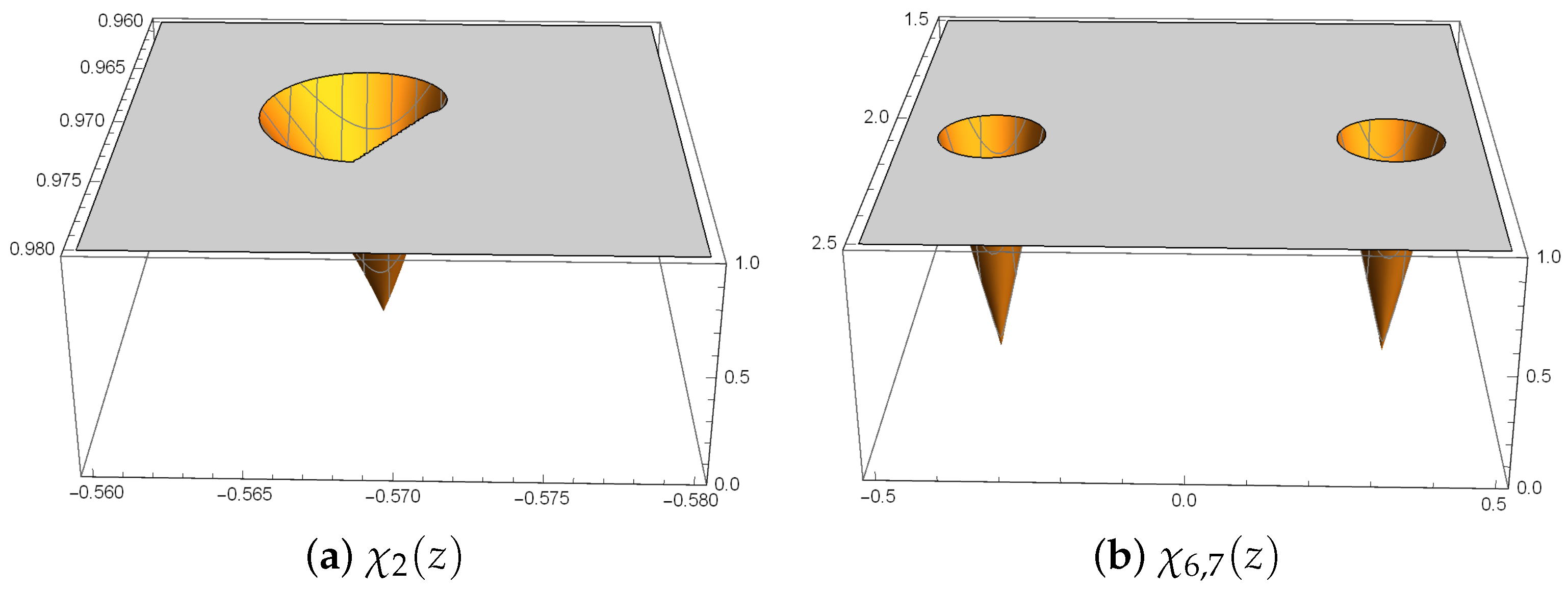
- is an attractor for values of α in small regions of the complex plane, inside the complex area .
- •
- is an attractor for values of α in small regions of the complex plane, inside the complex area .
3.3. Critical Points of Operator
- •
- If , then has three different free critical points (with multiplicity 8), . If , , then has four different free critical points (with multiplicity 4), (with multiplicity 4), .
- •
- If , , then has three different free critical points (with multiplicity 4), .
- •
- If , , has five different free critical points (with multiplicity 2), . If , there are six different free critical points .
- •
- If , there are three different free critical points (with multiplicity 4), ; and with , there are five different free critical points (with multiplicity 4), .
- •
- For , there are seven different free critical pointswhere Moreover, it can be proved that all free critical points are not independent, as
3.4. Parameter Spaces and Dynamical Planes
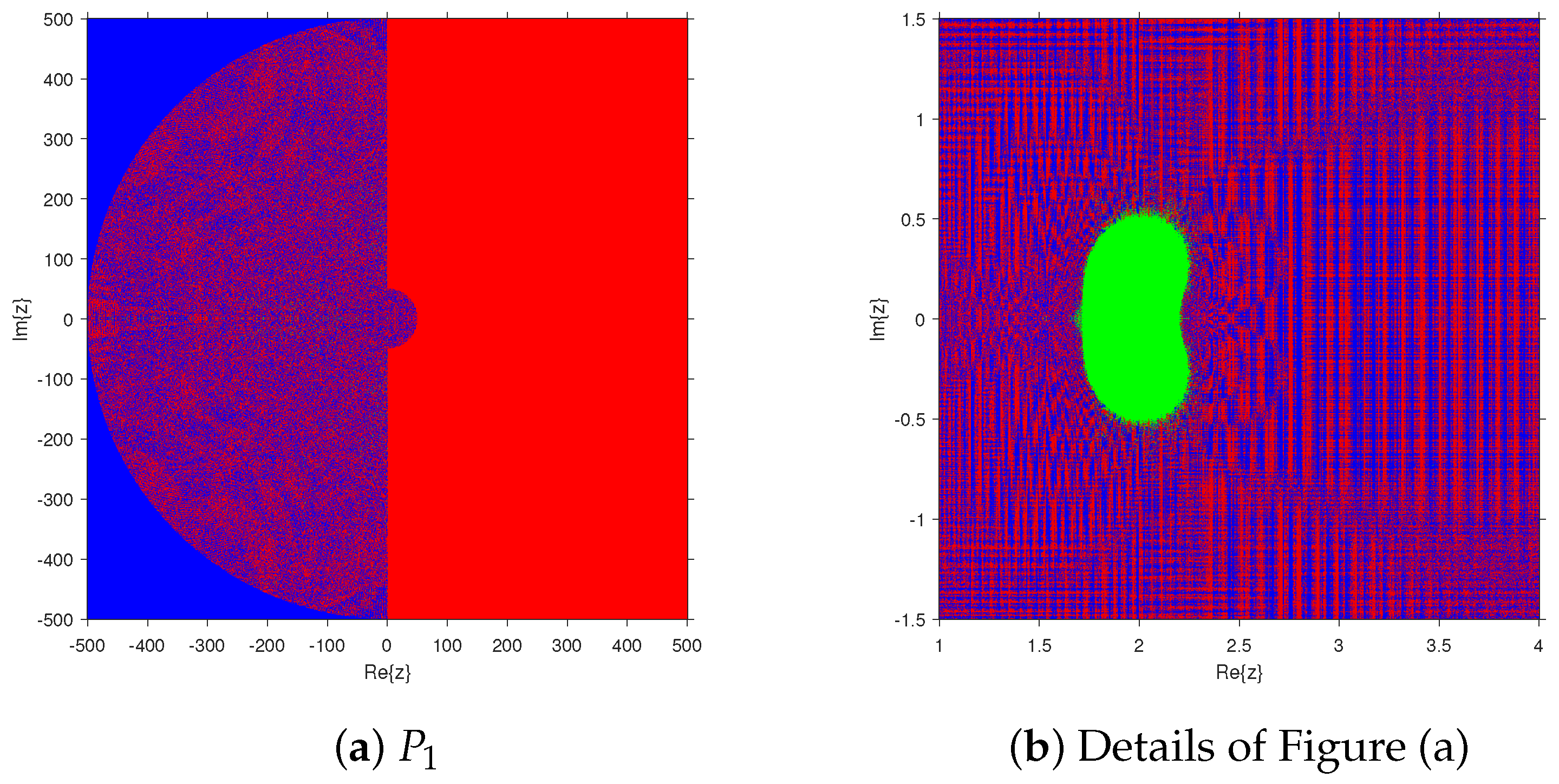
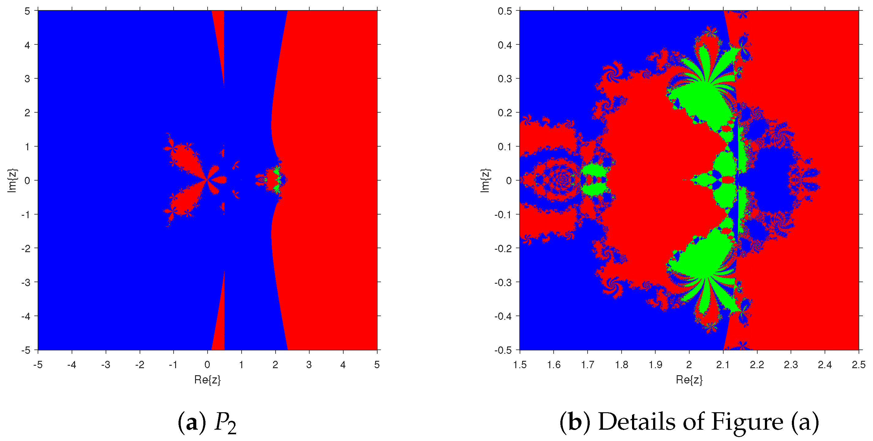
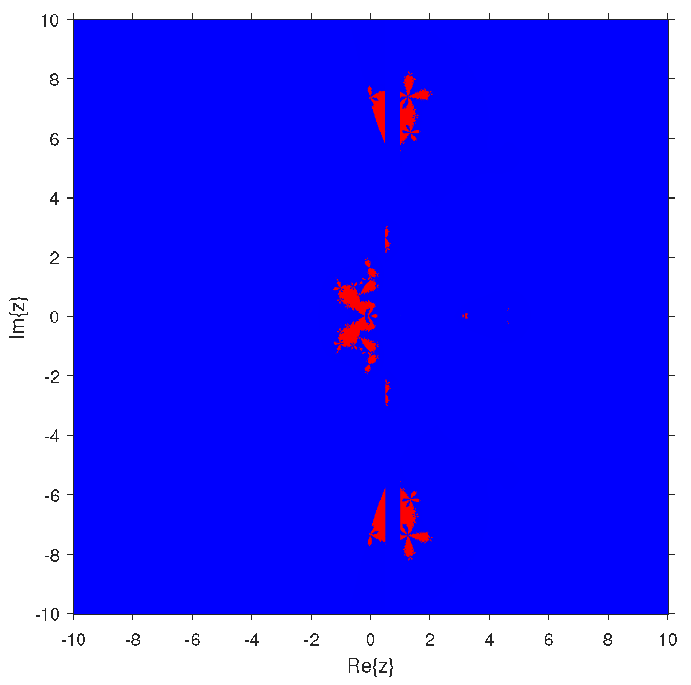
3.4.1. Parameter Spaces
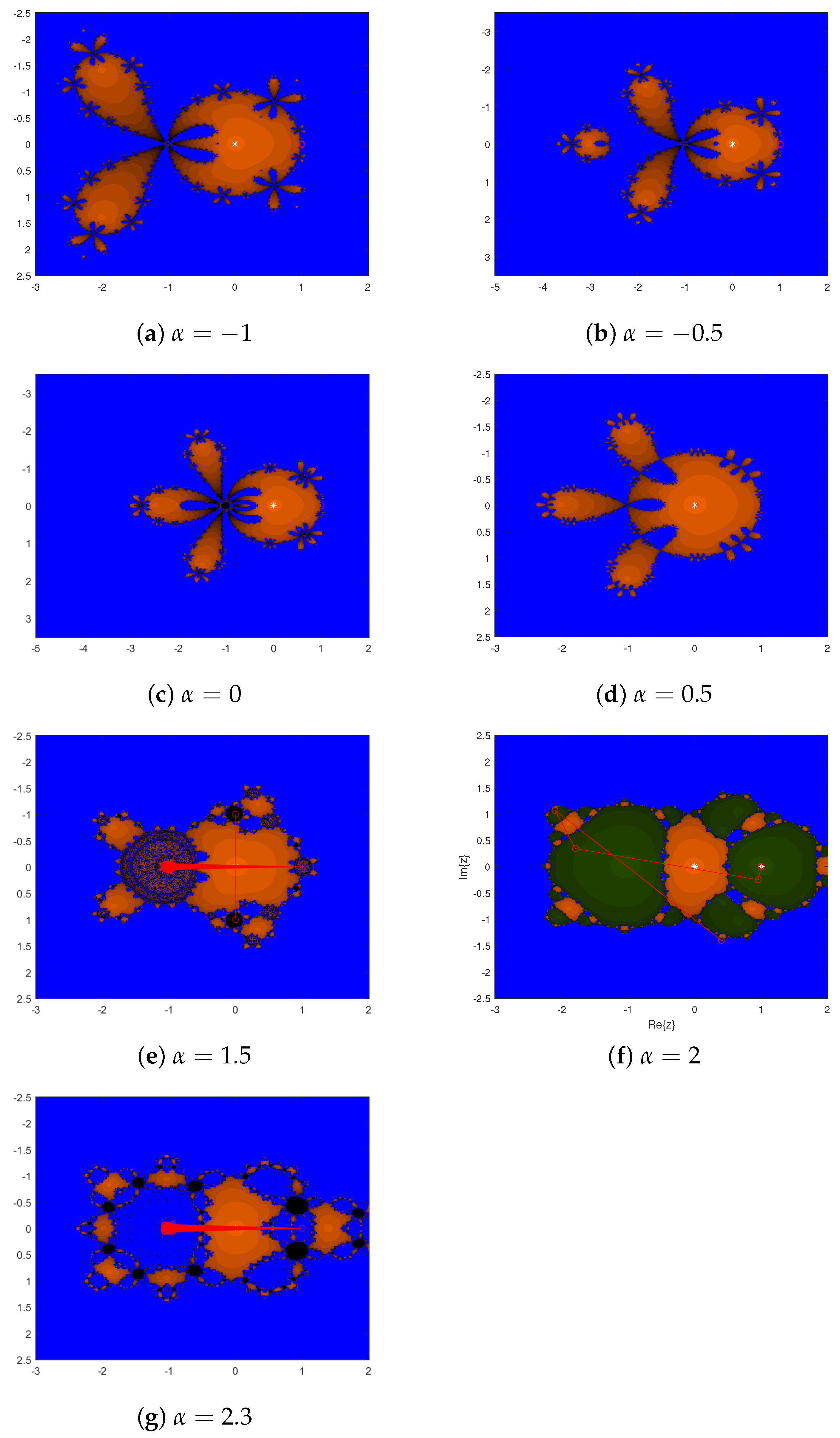
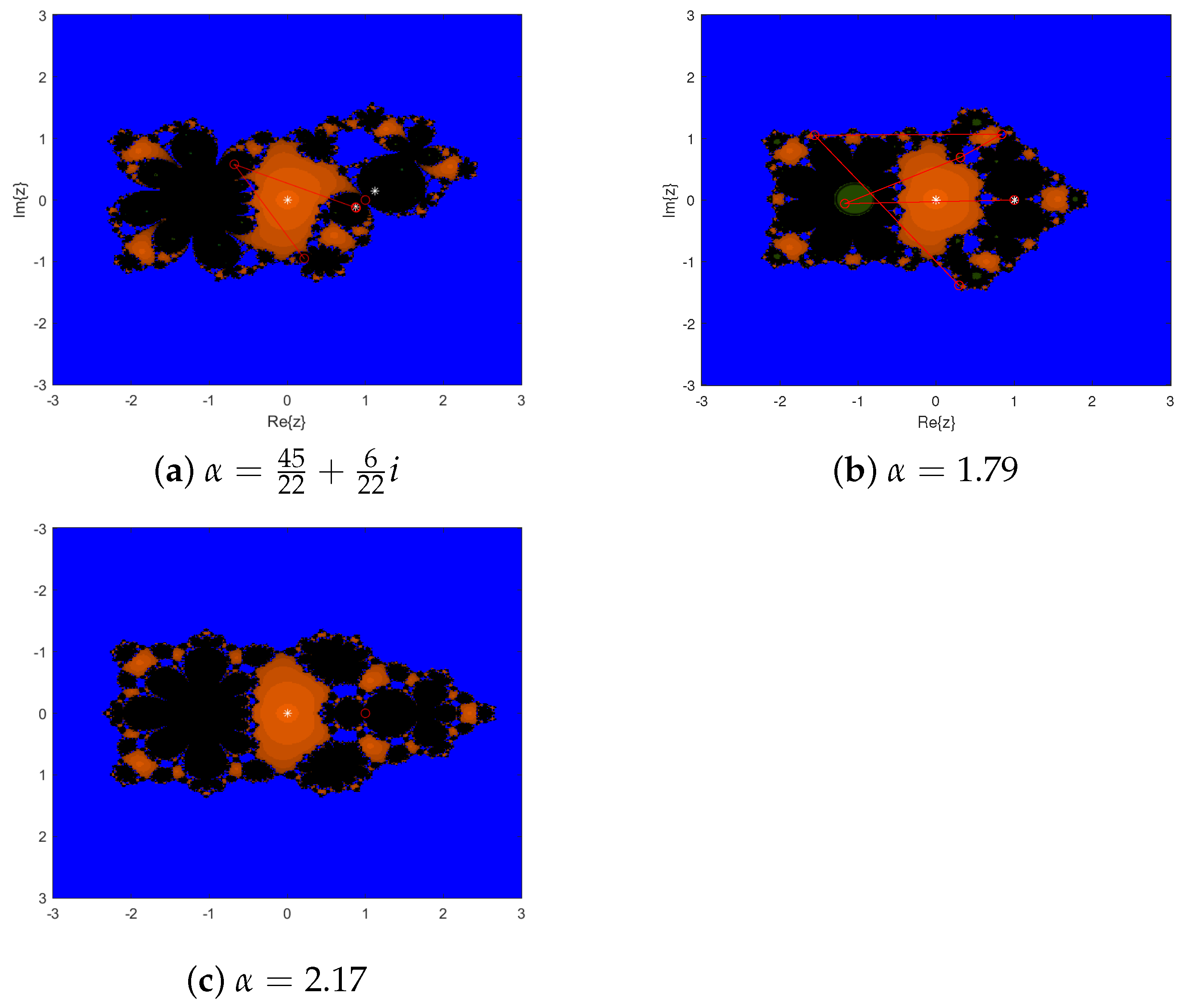
3.4.2. Dynamical Planes
4. Numerical Experiments
- •
- •
- In addition, let us consider a physical problem. An object of mass m is dropped from a height h onto a real spring whose elastic force is , where z is the compression of the spring; calculate the maximum compression of the spring:Let the gravity be , the proportionality constant , , mass of the object and height . Thus, we obtain the test function.
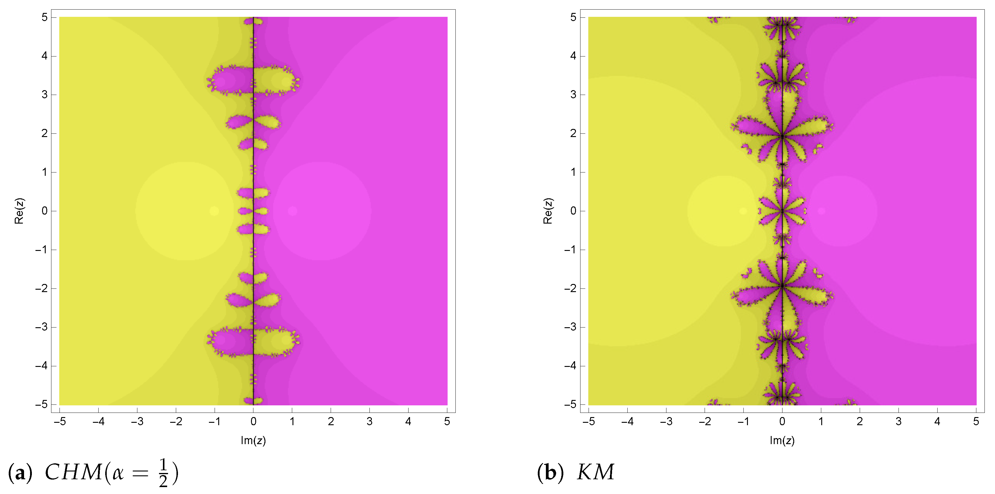
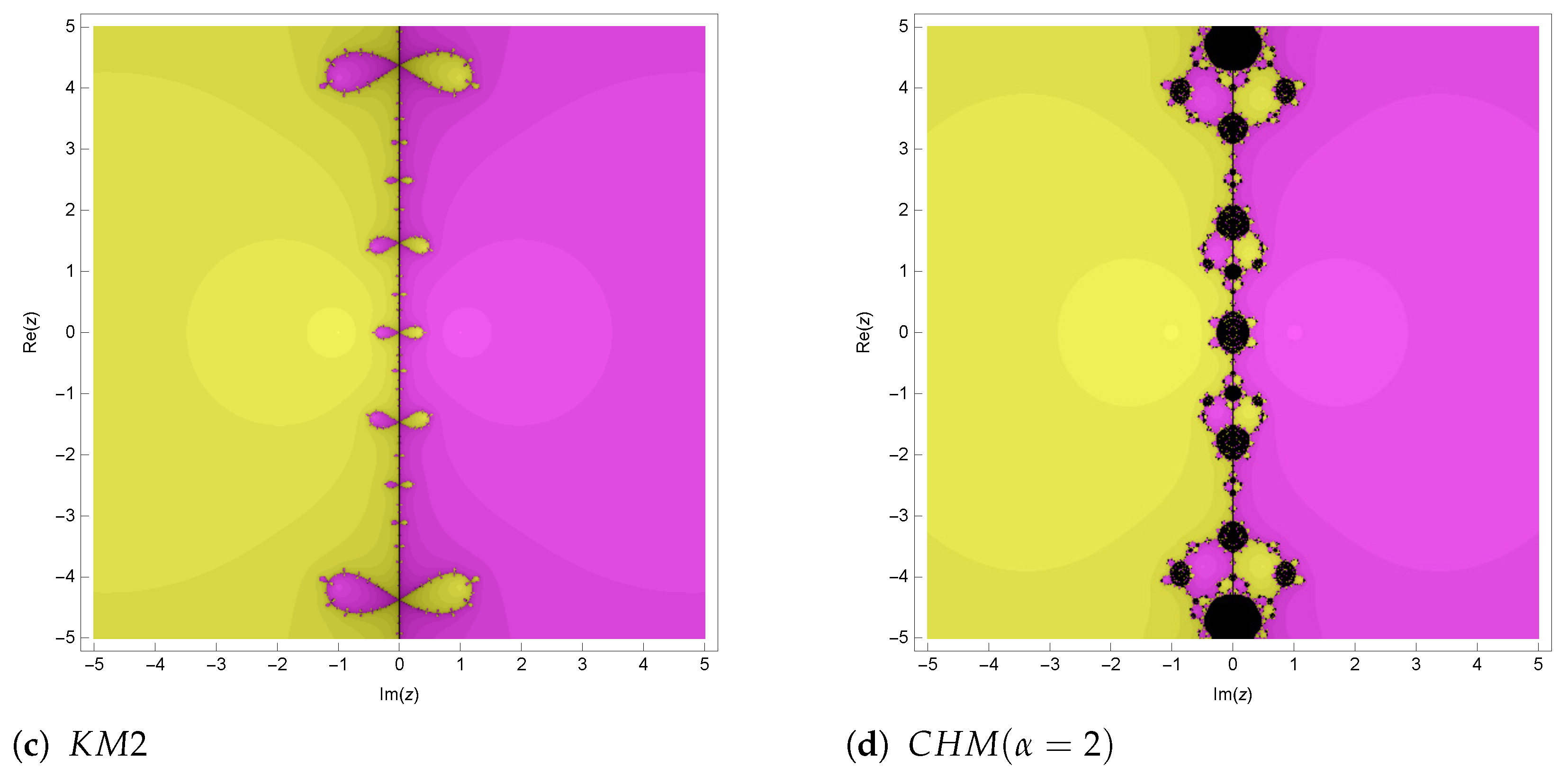
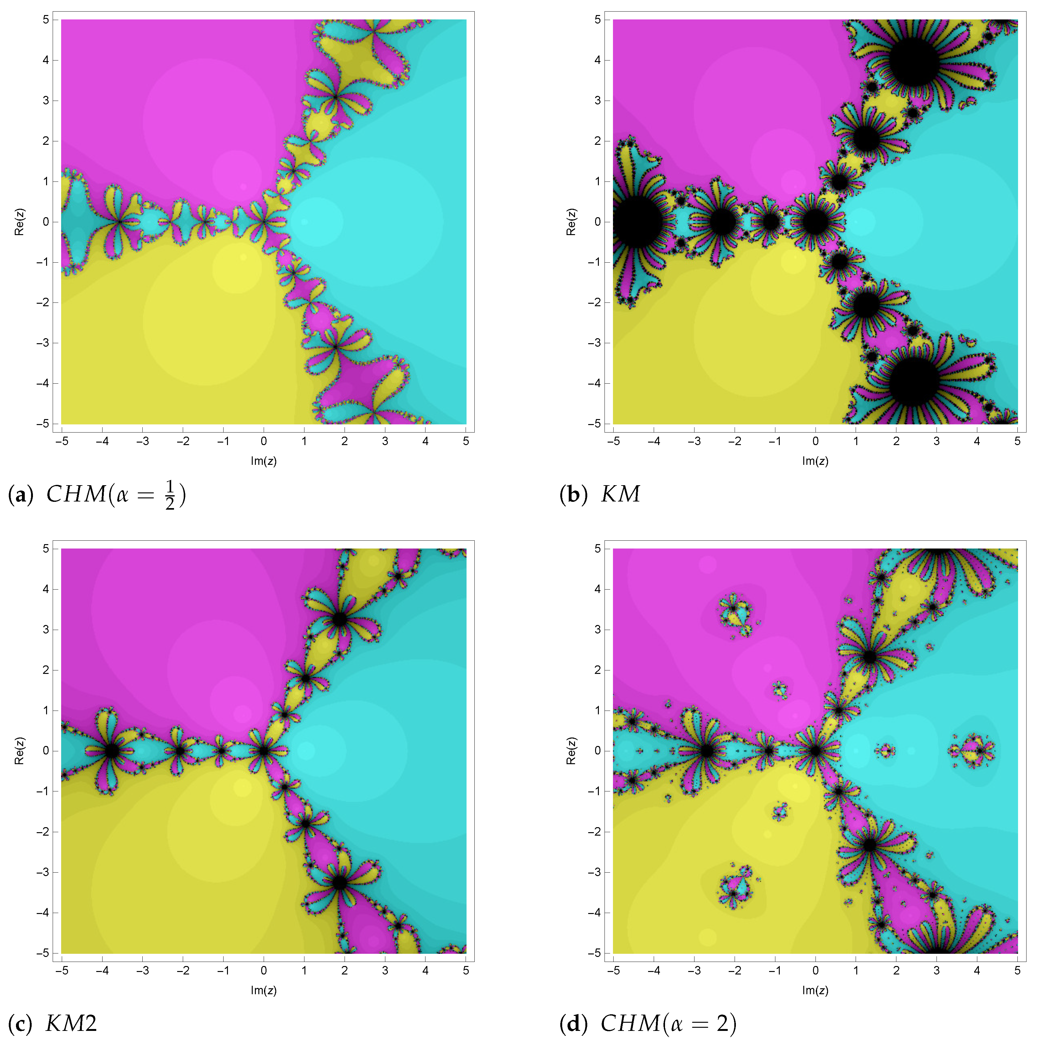
5. Comparison of Fractal Diagram for Different Methods
6. Conclusions
Author Contributions
Funding
Data Availability Statement
Acknowledgments
Conflicts of Interest
References
- Ortega, J.M.; Rheinboldt, W.C. Iterative Solution of Nonlinear Equations in Several Variables; SIAM: Philadelphia, PA, USA, 2000. [Google Scholar]
- Steffensen, J.F. Remarks on iteration. Scand. Actuar. J. 1933, 1933, 64–72. [Google Scholar] [CrossRef]
- Jarratt, P. Some fourth order multipoint iterative methods for solving equations. Math. Comput. 1966, 20, 434–437. [Google Scholar] [CrossRef]
- Ostrowski, A.M. Solution of Equations in Euclidean and Banach Spaces; Academic Press: Cambridge, MA, USA, 1973. [Google Scholar]
- Werner, W. Some improvements of classical iterative methods for the solution of nonlinear equations. In Numerical Solution of Nonlinear Equations: Proceedings Bremen; Springer: Berlin/Heidelberg, Germany, 1980; pp. 426–440. [Google Scholar]
- Singh, H.; Akhavan Ghassabzadeh, F.; Tohidi, E.; Cattani, C. Legendre spectral method for the fractional Bratu problem. Math. Methods. Appl. Sci. 2020, 43, 5941–5952. [Google Scholar] [CrossRef]
- Nachaoui, A. An iterative method for cauchy problems subject to the convection-diffusion equation. Adv. Math. Models Appl. 2023, 8, 327–338. [Google Scholar]
- Sihwail, R.; Solaiman, O.S.; Ariffin, K.A.Z. New robust hybrid Jarratt-Butterfly optimization algorithm for nonlinear models. J. King Saud. Univ.-Comput. Inf. Sci. 2022, 34, 8207–8220. [Google Scholar] [CrossRef]
- Said Solaiman, O.; Sihwail, R.; Shehadeh, H.; Hashim, I.; Alieyan, K. Hybrid Newton–Sperm Swarm Optimization Algorithm for Nonlinear Systems. Mathematics 2023, 11, 1473. [Google Scholar] [CrossRef]
- Kou, J.; Li, Y. The improvements of Chebyshev–Halley methods with fifth-order convergence. Appl. Math. Comput. 2007, 188, 143–147. [Google Scholar] [CrossRef]
- Li, D.; Liu, P.; Kou, J. An improvement of Chebyshev–Halley methods free from second derivative. Appl. Math. Comput. 2014, 235, 221–225. [Google Scholar] [CrossRef]
- Chun, C. Some second-derivative-free variants of Chebyshev–Halley methods. Appl. Math. Comput. 2007, 191, 410–414. [Google Scholar] [CrossRef]
- Kou, J. On Chebyshev–Halley methods with sixth-order convergence for solving non-linear equations. Appl. Math. Comput. 2007, 190, 126–131. [Google Scholar] [CrossRef]
- Kim, Y.I.; Behl, R.; Motsa, S.S. Higher-order efficient class of Chebyshev–Halley-type methods. Appl. Math. Comput. 2016, 273, 1148–1159. [Google Scholar] [CrossRef]
- Cordero, A.; Torregrosa, J.R.; Vindel, P. Dynamics of a family of Chebyshev–Halley-type methods. Appl. Math. Comput. 2013, 219, 8568–8583. [Google Scholar] [CrossRef]
- Chicharro, F.I.; Cordero, A.; Torregrosa, J.R. Drawing dynamical and parameters planes of iterative families and methods. Sci. World. J. 2013, 2013, 780153. [Google Scholar] [CrossRef] [PubMed]
- Cordero, A.; Jaiswal, J.P.; Torregrosa, J.R. Stability analysis of fourth-order iterative method for finding multiple roots of non-linear equations. Appl. Math. Nonlinear Sci. 2019, 4, 43–56. [Google Scholar] [CrossRef]
- Behl, R.; Cordero, A.; Motsa, S.S.; Torregrosa, J.R. On optimal fourth-order optimal families of methods for multiple roots and their dynamics. Appl. Math. Comput. 2015, 265, 520–532. [Google Scholar] [CrossRef]
- Cordero, A.; Moscoso-Martínez, M.; Torregrosa, J.R. Chaos and stability in a new iterative family for solving nonlinear equations. Algorithms 2021, 14, 101. [Google Scholar] [CrossRef]
- Lee, M.Y.; Kim, Y.I. The dynamical analysis of a uniparametric family of three-point optimal eighth-order multiple-root finders under the Möbius conjugacy map on the Riemann sphere. Numer. Algorithms 2020, 83, 1063–1090. [Google Scholar] [CrossRef]
- Wang, X.; Chen, X. The dynamical analysis of a biparametric family of six-order Ostrowski-type method under the Möbius conjugacy map. Fractal Fract. 2022, 6, 174. [Google Scholar] [CrossRef]
- Wang, X.; Chen, X.; Li, W. Dynamical behavior analysis of an eighth-order Sharma’s method. Int. J. Biomath. 2023, 2350068. [Google Scholar] [CrossRef]
- Wang, X.; Xu, J. Conformable vector Traub’s method for solving nonlinear systems. Numer. Algorithms 2024. [Google Scholar] [CrossRef]
- Falconer, K. Fractal Geometry: Mathematical Foundations and Applications; John Wiley & Sons: Hoboken, NJ, USA, 1990. [Google Scholar]
- Mandelbrot, B.B. Fractal geometry: What is it, and what does it do? Proc. Math. Phys. Eng. Sci. 1989, 423, 3–16. [Google Scholar]
- Cordero, A.; Torregrosa, J.R. Variants of Newton’s method using fifth-order quadrature formulas. Appl. Math. Comput. 2007, 190, 686–698. [Google Scholar] [CrossRef]
- Kou, J.; Li, Y. Modified Chebyshev’s method free from second derivative for non-linear equations. Appl. Math. Comput. 2007, 187, 1027–1032. [Google Scholar] [CrossRef]


| Method | ACOC | Time | ||||||
|---|---|---|---|---|---|---|---|---|
| CHM | 0.2 | 0.05753 | 2.8768 | 1.1312 | 1.0635 | 5.0 | 0.368283 | |
| KM | 0.2 | 0.05753 | 4.9599 | 2.6574 | 1.1731 | 5.0 | 0.504487 | |
| LIM | 0.2 | 0.05753 | 4.2069 | 7.8807 | 1.8179 | 5.0 | 0.685724 | |
| CHM | 0.3 | 0.04247 | 9.2906 | 3.9736 | 5.687 | 5.0 | 0.465012 | |
| KM | 0.3 | 0.04247 | 1.3287 | 3.6658 | 5.8604 | 5.0 | 0.700821 | |
| LIM | 0.3 | 0.04247 | 7.5548 | 1.4718 | 4.1309 | 5.0 | 0.617231 | |
| CHM | 1.3 | 0.06523 | 3.2362 | 8.0437 | 7.6303 | 5.0 | 0.495794 | |
| KM | 1.3 | 0.065231 | 9.2698 | 4.6694 | 1.5142 | 5.0 | 0.553354 | |
| LIM | 1.3 | 0.06523 | 1.6599 | 2.2011 | 9.0229 | 5.0 | 0.550163 | |
| CHM | 1.4 | 0.03477 | 1.0435 | 2.8031 | 3.9216 | 5.0 | 0.360747 | |
| KM | 1.4 | 0.03477 | 3.2389 | 2.4315 | 5.7982 | 5.0 | 0.417446 | |
| LIM | 1.4 | 0.03477 | 1.0054 | 1.7939 | 3.245 | 5.0 | 0.498558 | |
| CHM | 1.5 | 0.025994 | 4.5845 | 6.9123 | 5.3858 | 5.0 | 0.480012 | |
| KM | 1.5 | 0.025994 | 1.7726 | 2.4137 | 1.13 | 5.0 | 0.481797 | |
| LIM | 1.5 | 0.025994 | 5.9101 | 4.1989 | 7.6005 | 5.0 | 0.796286 | |
| CHM | 1.6 | 0.074001 | 5.3941 | 1.5586 | 3.139 | 4.9999995 | 0.524147 | |
| KM | 1.6 | 0.074032 | 0.000025903 | 1.6086 | 1.4855 | 5.0000019 | 0.484185 | |
| LIM | 1.6 | 0.073982 | 0.000023806 | 4.4536 | 1.0203 | 5.0000038 | 1.117498 | |
| CHM | 1.4 | 0.0044916 | 3.356 | 7.6642 | 4.761 | 5.0 | 0.384553 | |
| KM | 1.4 | 0.0044916 | 8.3785 | 1.8583 | 9.9733 | 5.0 | 0.363025 | |
| LIM | 1.4 | 0.0044916 | 1.1576 | 1.3428 | 2.8203 | 5.0 | 0.514793 | |
| CHM | 1.5 | 0.095499 | 9.5656 | 1.4419 | 1.1219 | 4.9999991 | 0.676156 | |
| KM | 1.5 | 0.095533 | 0.000024869 | 4.2817 | 6.4769 | 5.0000024 | 0.744585 | |
| LIM | 1.5 | 0.0955 | 8.5631 | 2.9745 | 1.5044 | 5.0000008 | 1.075170 | |
| CHM | −0.4 | 0.042854 | 5.0183 | 1.1955 | 9.174 | 5.0 | 0.544822 | |
| KM | −0.4 | 0.042855 | 3.6043 | 1.5472 | 2.2556 | 5.0 | 0.572932 | |
| LIM | −0.4 | 0.042854 | 3.1056 | 4.9815 | 5.2894 | 5.0 | 0.730796 | |
| CHM | −0.5 | 0.057145 | 2.5432 | 3.9964 | 3.8292 | 5.0 | 0.763921 | |
| KM | −0.5 | 0.057147 | 1.6222 | 2.8576 | 4.847 | 5.0 | 0.585273 | |
| LIM | −0.5 | 0.057145 | 8.2965 | 6.7774 | 2.4655 | 4.9999999 | 0.753026 | |
| CHM | 0.1 | 0.055438 | 0.011285 | 2.2307 | 4.8967 | 5.0293972 | 0.793084 | |
| KM | 0.1 | 0.091476 | 0.024762 | 0.000010038 | 1.8075 | 4.9362619 | 0.837225 | |
| LIM | 0.1 | 0.067567 | 0.00084373 | 3.1209 | 9.2141 | 5.1198554 | 0.933355 | |
| CHM | 0.2 | 0.033261 | 0.000015741 | 8.5645 | 4.0847 | 4.9999885 | 0.861654 | |
| KM | 0.2 | 0.033315 | 0.000038138 | 1.4321 | 1.0684 | 5.000026 | 1.014709 | |
| LIM | 0.2 | 0.03326 | 0.000016127 | 4.8457 | 8.3149 | 5.007914 | 1.187511 |
| ACOC | Time | |||||||
|---|---|---|---|---|---|---|---|---|
| −1 | 0.3 | 0.04247 | 5.1534 | 9.5535 | 2.0917 | 5.0 | 0.533905 | |
| 0.3 | 0.04247 | 6.542 | 4.3928 | 5.9965 | 5.0 | 0.353646 | ||
| 0.3 | 0.04247 | 9.2906 | 3.9736 | 5.687 | 5.0 | 0.457915 | ||
| −1 | 1 | 0.73694 | 0.0055298 | 1.4278 | 1.5599 | 5.0018483 | 1.203424 | |
| 1 | 0.73644 | 0.00603 | 3.0361 | 9.4566 | 5.0014638 | 0.654055 | ||
| 1 | 0.7352 | 0.0072671 | 1.1962 | 1.4062 | 5.0011154 | 0.574249 | ||
| -1 | 1.4 | 0.03477 | 4.8832 | 3.1527 | 3.5361 | 5.0 | 0.455763 | |
| 1.4 | 0.03477 | 3.6526 | 5.4119 | 3.8648 | 5.0 | 0.420997 | ||
| 1.4 | 0.03477 | 1.0435 | 2.8031 | 3.9216 | 5.0 | 0.736641 | ||
| −1 | 2 | 0.62288 | 0.011886 | 2.5419 | 1.2049 | 4.9967226 | 0.476672 | |
| 2 | 0.62437 | 0.010403 | 9.7005 | 7.1504 | 4.9975948 | 0.429954 | ||
| 2 | 0.62983 | 0.0049369 | 6.5529 | 2.738 | 4.9993795 | 0.482312 | ||
| −1 | 1.5 | 0.025994 | 3.1251 | 6.1457 | 1.8076 | 5.0000001 | 0.505113 | |
| 1.5 | 0.025994 | 2.1731 | 7.2122 | 2.9043 | 5.0 | 0.600533 | ||
| 1.5 | 0.025994 | 4.5845 | 6.9123 | 5.3858 | 5.0 | 0.412318 | ||
| −1 | 2 | 0.44736 | 0.026644 | 2.1889 | 1.036 | 4.9799307 | 0.540150 | |
| 2 | 0.44988 | 0.024127 | 1.0121 | 1.5806 | 4.9851187 | 0.472520 | ||
| 2 | 0.46174 | 0.01227 | 8.9598 | 1.9708 | 4.9964929 | 0.584135 | ||
| −1 | 1.4 | 0.0044916 | 1.5364 | 6.9365 | 1.301 | 5.0 | 0.763457 | |
| 1.4 | 0.0044916 | 1.1328 | 1.1194 | 1.0548 | 5.0 | 0.778445 | ||
| 1.4 | 0.0044916 | 3.356 | 7.6642 | 4.761 | 5.0 | 0.457384 | ||
| −1 | 1 | nc | nc | nc | nc | nc | nc | |
| 1 | nc | nc | nc | nc | nc | nc | ||
| 1 | 0.27406 | 0.13031 | 0.00012133 | 4.7358 | 5.083647 | 0.822961 | ||
| −1 | -0.4 | 0.042854 | 3.8978 | 2.9643 | 7.541 | 5.0 | 0.550584 | |
| -0.4 | 0.042854 | 2.8444 | 4.3227 | 3.5043 | 5.0 | 0.573988 | ||
| -0.4 | 0.042854 | 5.0183 | 1.1955 | 9.174 | 5.0 | 0.352655 | ||
| −1 | 0 | 0.43258 | 0.010278 | 3.5974 | 1.9851 | 4.9971435 | 0.502055 | |
| 0 | 0.43396 | 0.0088947 | 1.2485 | 7.0433 | 4.9980779 | 0.498097 | ||
| 0 | 0.43998 | 0.0028767 | 7.3611 | 8.1186 | 4.9997831 | 0.479472 | ||
| −1 | 0.1 | nc | nc | nc | nc | nc | nc | |
| 0.1 | nc | nc | nc | nc | nc | nc | ||
| 0.1 | 0.055438 | 0.011285 | 2.2307 | 4.8967 | 5.0293972 | 0.793084 | ||
| −1 | 0.2 | 0.033233 | 0.000043824 | 5.7218 | 2.1749 | 4.9999423 | 0.974917 | |
| 0.2 | 0.03324 | 0.000036187 | 1.6483 | 3.2357 | 4.9999586 | 1.016791 | ||
| 0.2 | 0.033261 | 0.000015741 | 8.5645 | 4.0847 | 4.9999885 | 0.861654 |
| ACOC | Time | |||||||
|---|---|---|---|---|---|---|---|---|
| 1.5 | 0.3 | 0.04247 | 1.2001 | 1.9459 | 2.1807 | 5.0 | 0.636435 | |
| 2 | 0.3 | 0.04247 | 1.3343 | 3.7441 | 6.5139 | 5.0 | 0.622020 | |
| 2.17 | 0.3 | 0.04247 | 1.3797 | 4.6023 | 1.9009 | 5.0 | 0.516650 | |
| 1.5 | 1 | 0.7335 | 0.0089677 | 4.6371 | 1.6756 | 5.0009595 | 0.632580 | |
| 2 | 1 | 0.73239 | 0.010082 | 9.4161 | 6.5534 | 5.0009115 | 0.541331 | |
| 2.17 | 1 | 0.73196 | 0.010515 | 1.2077 | 2.3649 | 5.0008979 | 0.526807 | |
| 1.5 | 1.4 | 0.03477 | 1.7826 | 6.8271 | 5.6248 | 5.0 | 0.383288 | |
| 2 | 1.4 | 0.03477 | 3.2854 | 2.6113 | 8.2829 | 5.0 | 0.387603 | |
| 2.17 | 1.4 | 0.03477 | 3.8109 | 6.3115 | 7.8636 | 5.0 | 0.388549 | |
| 1.5 | 2 | 0.64754 | 0.012775 | 1.3287 | 1.5705 | 5.0015962 | 0.371706 | |
| 2 | 2 | 0.68237 | 0.047599 | 1.8055 | 1.3087 | 5.0064011 | 0.401961 | |
| 2.17 | 2 | 0.71315 | 0.078385 | 2.6199 | 9.6917 | 5.0116522 | 0.390029 | |
| 1.5 | 1.5 | 0.025994 | 1.0419 | 9.8946 | 7.6415 | 5.0 | 0.509447 | |
| 2 | 1.5 | 0.025994 | 1.7237 | 2.0986 | 5.6139 | 5.0 | 0.545617 | |
| 2.17 | 1.5 | 0.025994 | 1.9461 | 4.3943 | 2.5795 | 5.0 | 0.473363 | |
| 1.5 | 2 | 0.56001 | 0.086052 | 0.000051492 | 2.9164 | 5.0408977 | 0.488337 | |
| 2 | 2 | nc | nc | nc | nc | nc | nc | |
| 2.17 | 2 | nc | nc | nc | nc | nc | nc | |
| 1.5 | 1.4 | 0.0044916 | 4.4841 | 4.3515 | 3.7449 | 5.0 | 0.709110 | |
| 2 | 1.4 | 0.0044916 | 8.3557 | 1.8331 | 9.3145 | 5.0 | 0.705258 | |
| 2.17 | 1.4 | 0.0044916 | 9.6647 | 4.3973 | 8.5733 | 5.0 | 0.699666 | |
| 1.5 | 1 | 0.64393 | 0.23998 | 0.00054848 | 1.1945 | 4.7943402 | 0.688360 | |
| 2 | 1 | 0.72825 | 0.32888 | 0.0051229 | 1.6162 | 4.7031415 | 0.879573 | |
| 2.17 | 1 | 0.75033 | 0.35501 | 0.0091719 | 3.4807 | 4.6736711 | 0.745030 | |
| 1.5 | -0.4 | 0.042855 | 2.2154 | 8.3805 | 6.4923 | 5.0 | 0.490509 | |
| 2 | -0.4 | 0.042855 | 3.7423 | 1.867 | 5.7706 | 5.0 | 0.499436 | |
| 2.17 | -0.4 | 0.042855 | 4.2904 | 4.179 | 3.6639 | 5.0 | 0.737970 | |
| 1.5 | 0 | 0.4731 | 0.03025 | 4.0617 | 1.7361 | 5.0015384 | 0.459926 | |
| 2 | 0 | 0.69565 | 0.25573 | 0.0029359 | 5.553 | 5.0118838 | 0.470911 | |
| 2.17 | 0 | nc | nc | nc | nc | nc | nc | |
| 1.5 | 0.1 | 0.042855 | 0.012147 | 1.727 | 1.3621 | 4.9725788 | 1.238945 | |
| 2 | 0.1 | 0.084431 | 0.01771 | 2.215 | 9.4549 | 4.9629725 | 1.001502 | |
| 2.17 | 0.1 | 0.085903 | 0.019183 | 3.8987 | 1.869 | 4.9618955 | 1.055451 | |
| 1.5 | 0.2 | 0.033293 | 0.000016401 | 1.0528 | 1.1468 | 5.0000115 | 1.223707 | |
| 2 | 0.2 | 0.033317 | 0.000040334 | 1.8947 | 4.3301 | 5.0000249 | 1.158187 | |
| 2.17 | 0.2 | 0.033327 | 0.000050322 | 6.7019 | 2.8053 | 5.0000295 | 1.150161 |
Disclaimer/Publisher’s Note: The statements, opinions and data contained in all publications are solely those of the individual author(s) and contributor(s) and not of MDPI and/or the editor(s). MDPI and/or the editor(s) disclaim responsibility for any injury to people or property resulting from any ideas, methods, instructions or products referred to in the content. |
© 2024 by the authors. Licensee MDPI, Basel, Switzerland. This article is an open access article distributed under the terms and conditions of the Creative Commons Attribution (CC BY) license (https://creativecommons.org/licenses/by/4.0/).
Share and Cite
Wang, X.; Guo, S. A Class of Fifth-Order Chebyshev–Halley-Type Iterative Methods and Its Stability Analysis. Fractal Fract. 2024, 8, 150. https://doi.org/10.3390/fractalfract8030150
Wang X, Guo S. A Class of Fifth-Order Chebyshev–Halley-Type Iterative Methods and Its Stability Analysis. Fractal and Fractional. 2024; 8(3):150. https://doi.org/10.3390/fractalfract8030150
Chicago/Turabian StyleWang, Xiaofeng, and Shaonan Guo. 2024. "A Class of Fifth-Order Chebyshev–Halley-Type Iterative Methods and Its Stability Analysis" Fractal and Fractional 8, no. 3: 150. https://doi.org/10.3390/fractalfract8030150