Article

A Matrix Transform Technique for Distributed-Order Time-Fractional Advection–Dispersion Problems

by
Mohammadhossein Derakhshan
1,2,
Ahmed S. Hendy
3,4,
António M. Lopes
5,
Alexandra Galhano
6,* and
Mahmoud A. Zaky
7
1
Department of Industrial Engineering, Apadana Institute of Higher Education, Shiraz 7187985443, Iran
2
Faculty of Technology and Engineering, Zand Institute of Higher Education, Shiraz 8415683111, Iran
3
Computational Mathematics and Computer Science, Institute of Natural Sciences and Mathematics, Ural Federal University, 19 Mira St., Yekaterinburg 620002, Russia
4
Department of Mathematics, Faculty of Science, Benha University, Benha 13511, Egypt
5
LAETA/INEGI, Faculty of Engineering, University of Porto, Rua Dr. Roberto Frias, 4200-465 Porto, Portugal
6
Faculdade de Ciências Naturais, Engenharias e Tecnologias, Universidade Lusófona do Porto, Rua de Augusto Rosa 24, 4000-098 Porto, Portugal
7
Department of Mathematics and Statistics, College of Science, Imam Mohammad Ibn Saud Islamic University (IMSIU), Riyadh 13318, Saudi Arabia
*
Author to whom correspondence should be addressed.
Fractal Fract. 2023, 7(9), 649; https://doi.org/10.3390/fractalfract7090649
Submission received: 19 June 2023 / Revised: 19 August 2023 / Accepted: 22 August 2023 / Published: 25 August 2023
(This article belongs to the Section Mathematical Physics)

Abstract

:
Invoking the matrix transfer technique, we propose a novel numerical scheme to solve the time-fractional advection–dispersion equation (ADE) with distributed-order Riesz-space fractional derivatives (FDs). The method adopts the midpoint rule to reformulate the distributed-order Riesz-space FDs by means of a second-order linear combination of Riesz-space FDs. Then, a central difference approximation is used side by side with the matrix transform technique for approximating the Riesz-space FDs. Based on this, the distributed-order time-fractional ADE is transformed into a time-fractional ordinary differential equation in the Caputo sense, which has an equivalent Volterra integral form. The Simpson method is used to discretize the weakly singular kernel of the resulting Volterra integral equation. Stability, convergence, and error analysis are presented. Finally, simulations are performed to substantiate the theoretical findings.

1. Introduction

In recent years, the theory and applications of derivatives and integrals of fractional order have played an important role in many fields [1,2,3,4,5,6,7]. Anomalous relaxation is well explained in many complex systems using multi-term fractional order models. As a result, multi-term partial differential equations (PDEs) of fractional order have found widespread application in describing real-world physical phenomena, as is the case of anomalous diffusive effects, damping, magnetic resonance imaging, and the mechanical and physical behavior of oxygen transport through capillaries [8,9,10]. In [11], the concept of distributed-order fractional operators and, recently, distributed-order fractional PDEs, have been generalized. However, the distributed order FDs constitute a topic that is not new. Indeed, Caputo addressed such kind of operators in 1969, in the context of properties of inelastic media. The problem was solved in 1995 and, later, in [12], a viscoelastic model involving a multi-term FD was expanded to distributed order. FDs of distributed-order are operators that are integrated, within a specified range, over the order of differentiation. Fractional PDEs of distributed-order are an extension of single- and multi-term fractional PDEs [13,14,15]. Several authors have investigated various numerical approaches for solving fractional models of distributed order. Diethelm et al. [16] suggested an algorithm for approximating the solution of distributed-order differential equations. Ford et al. [17] used the implicit finite difference technique to provide an efficient numerical method to address the time distributed-order diffusion problem. For the time distributed-order Riesz-space FD model, Ye et al. [18] investigated an efficient numerical technique over bounded domains. Yang et al. [19] addressed a numerical strategy based on the WSGD-OSC technique for simulating the distributed order time fractional reaction-diffusion two-dimensional equation. Hu et al. [20] reported results of an implicit numerical approach for two-sided space- and distributed-order time-fractional ADEs. Zaky and Machado [21] proposed spectral tau approaches to solve the fractional diffusion problem with distributed-order with time and Dirichlet boundary conditions. Shi et al. [22] addressed an approach for the Riesz-space multi-term and distributed-order time-fractional wave equation based on the unstructured mesh finite element technique on an irregular convex domain. Aboelenen [23] developed a scheme based on the local discontinuous Galerkin finite element technique for solving distributed-order time- and Riesz-space-fractional PDEs. Chen et al. [24] proposed a finite difference/Laguerre spectral approximation for distributed-order time-fractional reaction-diffusion equations. Morgado et al. [25] introduced a Chebyshev collocation approach for providing approximate solutions to the distributed-order time-fractional diffusion equation. Zaky et al. [26] introduced a spectral Legendre collocation scheme for the initial fractional differential equation of distributed order. Fei and Huang [27] derived a Galerkin Legendre spectral technique for approximating the solution of time-fractional fourth-order distributed-order PDEs in two dimensions. The composite Simpson approach was used with the distributed-order integral term, whereas the L 2 1 method was adopted to approximate the multi-term order Caputo FDs. Zhang et al. analyzed a numerical approach for solving the two-dimensional distributed-order Riesz-space ADE using the Galerkin–Legendre spectral with the Crank–Nicolson alternating direction implicit method.
In this paper, the following time-fractional ADE with distributed-order Riesz-space FDs is considered:
C D t α z ( x , t ) = 1 2 κ ( p ) p z ( x , t ) x p d p + 1 2 κ ( q ) q z ( x , t ) x q d q + f ( x , t , z ) ,
with initial and boundary conditions (IBCs):
z ( 0 , t ) = h 1 ( t ) , z ( L , t ) = h 2 ( t ) , z ( x , 0 ) = f ( x ) ,
in which C D t α z ( x , t ) is the order α ( 0 , 1 ] Caputo derivative, and κ ( p ) and κ ( q ) are continuous weight functions satisfying
1 2 κ ( p ) d p = k 1 > 0 , 1 2 κ ( q ) d q = k 2 > 0 .
Also, ζ z ( x , t ) x ζ stands for the order ζ ( 1 , 2 ] Riesz fractional operator, and h 1 ( t ) , h 2 ( t ) and f ( x ) are assumed continuous.
To obtain an approximation to (1), we employ stable numerical techniques based on the Simpson and finite difference methods. For this purpose, we use the finite difference scheme based on the matrix transform approach [28] to discretize the space-fractional ADE and the Simpson approach to discretize the time-fractional differential equations. To the best of our knowledge, this technique has not been used so far to approximate the solution of (1). We estimate the Riesz derivatives using the matrix transform approach, which converts (1) into a system of time-fractional differential equations. Finally, the Simpson scheme is employed for time-stepping, which avoids the need for solving nonlinear systems at each step. The theoretical convergence and the stability of the approximate solution are assessed. The advantage of using this new approach for the introduced problem is related to the fact that the numerical method includes simple calculations. Thus, the method is easy to simulate, and it is a powerful mathematical tool to compute the approximate solution of various types of models with little additional work. The proposed method can be used reliably and effectively to obtain approximate solutions for many types of models.
The organization of this paper is as mentioned in the following. In Section 2, some preliminary notions of fractional calculus are introduced. In Section 3, the numerical schemes for approximating the solution of (1) are proposed. Moreover, the error bound and stability are discussed. In Section 4, examples are given to report the accuracy and effectiveness of the new technique. Finally, some conclusions are provided in Section 5.

2. Preliminary Notions and Used Notation

We introduce definitions of fractional differentiation and integration of order θ ( n 1 , n ] , with n N , which are important in subsequent sections.
Definition 1
([2]). Let θ ( 0 , 1 ] . The Riemann-Liouville integral of order θ of a function u ( x , t ) is:
I t θ u ( x , t ) = 1 Γ ( θ ) 0 t ( t σ ) θ 1 u ( x , σ ) d σ .
Also, the Riemann–Liouville and Caputo FDs of order θ of u ( x , t ) are:
D t θ u ( x , t ) = d n d t n I t n θ u ( x , t ) , θ ( n 1 , n ] , n N { 0 } , C D t θ u ( x , t ) = I t n θ d n d t n u ( x , t ) .
Definition 2
([29]). The Riesz fractional differential operator of order θ ( n 1 , n ] over the finite interval [ 0 , L ] is:
θ u ( x , t ) | x | θ = K θ 0 D x θ + x D L θ u ( x , t ) ,
where
0 D x θ u ( x , t ) = 1 Γ ( n θ ) n x n 0 x ( x σ ) n θ 1 u ( σ , t ) d σ , x D L θ u ( x , t ) = 1 Γ ( n θ ) x L ( σ x ) n θ 1 u ( σ , t ) d σ ,
and K θ = 1 2 cos ( θ π 2 ) .
Definition 3
([30]). Let { ψ n } be the complete set of orthonormal eigenfunctions and λ n 2 be the corresponding eigenvalues for the Laplacian Δ over a bounded domain Ω, that is,
Δ ψ n = λ n 2 ψ n , o n Ω , B ( ψ ) = 0 , o n Ω ,
where B ( ψ ) is the given homogeneous boundary condition. Suppose that
F ρ = f = n = 1 f n ψ n , f n = f , ψ n : n = 1 | f n | 2 | λ | n ρ < , ρ = max ( α , 0 ) .
Then, for any given function f F ρ , Δ α 2 : F ρ L 2 ( Ω ) is described by:
Δ α 2 f = n = 1 f n λ n 2 α 2 ψ n .
Definition 4
([28]). Let { ψ n } be the complete set of orthonormal eigenfunctions and λ n 2 be the corresponding eigenvalues for the Laplacian Δ over a bounded domain Ω subject to the homogeneous boundary conditions. Then,
Δ α 2 f = Δ m f , i f α = 2 m , m = 0 , 1 , 2 , , Δ α 2 m Δ m f , i f m 1 < α 2 < m , m = 1 , 2 , , n = 1 λ n α f , ψ n ψ n , i f α < 0 .
Proposition 1
([2]). For a function f ( t ) and α ( n 1 , n ] , with n N , some practical and useful properties of the Caputo FD and Riemann–Liouville fractional integral are:
1. 
I t α ( C D t α f ( t ) ) = f ( t ) i = 0 n 1 f ( i ) ( 0 ) t i i ! , t > 0 ,
2. 
C D t α ( I t α f ( t ) ) = f ( t ) ,
3. 
C D t α t l = 0 , l < α , Γ ( l + 1 ) Γ ( l α + 1 ) t l α , l α ,
4. 
I t α I t α f ( t ) = I t α + α f ( t ) ,
5. 
I t α t l = Γ ( l + 1 ) Γ ( l + α + 1 ) t l + α .
Lemma 1
([31]). For the Riesz FD of order θ ( n 1 , n ] , with n N , and a given function u ( x , t ) over the infinite domain x , the next condition holds:
θ u ( x , t ) | x | θ = Δ θ 2 u ( x , t ) = K θ D x θ + x D θ u ( x , t ) .

3. Numerical Method

This section provides a numerical approach to solve (1) by applying the finite difference method via the matrix transform.
We use the midpoint approach to estimate the supplied integrals on the right-hand side of Equation (1), yielding
C D t α z ( x , t ) = 1 2 κ ( p ) 2 x 2 p 2 z ( x , t ) d p 1 2 κ ( q ) 2 x 2 q 2 z ( x , t ) d q + f ( x , t , z ) = 1 T i = 1 T κ ( p i ) 2 x 2 p i 2 z ( x , t ) 1 T j = 1 T κ ( q j ) 2 x 2 q j 2 z ( x , t ) + f ( x , t , z ) + O ( Δ σ ) 2 + O ( Δ σ ) 2 ,
where
1 = σ 0 < σ 1 < < σ T = 2 , Δ σ = 1 T , p i = σ i + σ i 1 2 , i = 1 , 2 , , T , 1 = σ 0 < σ 1 < < σ T = 2 , Δ σ = 1 T , q j = σ j + σ j 1 2 , j = 1 , 2 , , T .

3.1. Matrix Transform Method for Approximating the Riesz-Space Fractional Derivative

We use the matrix transform scheme introduced by Ilić [28] for approximating the Riesz-space FD, in order to spatially discretize the problem (1). First, we address the time-fractional ADE under the IBCs given in Equation (2):
C D t α z ( x , t ) = κ ( p ) 2 x 2 p 2 z ( x , t ) κ ( q ) 2 x 2 q 2 z ( x , t ) + f ( x , t , z ) .
Let x l = l Δ x , l = 0 , 1 , , n , Δ x = L n and z ( x l , t ) = z l ( t ) . Then, we apply the central difference method of second-order with respect to the space variable on the right side of Equation (12), to obtain
C D t α z l ( t ) = κ ( p ) δ x 2 ( Δ x ) 2 1 + δ x 2 12 + κ ( q ) δ x 2 ( Δ x ) 2 1 + δ x 2 12 z l ( t ) + f l ( t , z ) .
Thus, the matrix form of relation (13) can be obtained as:
C D t α Z ( t ) = κ ( p ) + κ ( q ) A 1 B ( Δ x ) 2 Z ( t ) + F ( t , Z ( t ) ) , Z ( 0 ) = Z 0 ,
where
Z ( t ) = [ z 1 ( t ) , z 2 ( t ) , , z n 1 ( t ) ] T , Z ( 0 ) = [ z 1 ( 0 ) , z 2 ( 0 ) , , z n 1 ( 0 ) ] T ,
and A and B are diagonally dominant matrices of size ( n 1 ) × ( n 1 ) given by
A = 5 6 1 12 0 0 0 1 12 5 6 1 12 0 0 0 1 12 5 6 1 12 0 0 1 12 5 6 1 12 0 0 0 1 12 5 6 1 12 0 0 0 1 12 5 6 ( n 1 ) × ( n 1 ) , B = 2 1 0 0 0 1 2 1 0 0 0 1 2 1 0 0 1 2 1 0 0 0 1 2 1 0 0 0 1 2 ( n 1 ) × ( n 1 ) .
As A and B are tridiagonal Toeplitz, then by using the definition of general tridiagonal Toeplitz matrix in [32], we have
A = Q Θ Q 1 , B = Q ˜ Θ ˜ Q ˜ 1 ,
and
Θ = diag λ 1 , λ 2 , , λ n 1 , Q = ς 1 , ς 2 , , ς n 1 , Θ ˜ = diag λ ˜ 1 , λ ˜ 2 , , λ ˜ n 1 , Q ˜ = ς ˜ 1 , ς ˜ 2 , , ς ˜ n 1 ,
in which λ v , λ ˜ v and ς v , ς ˜ v are the eigenvalues and eigenvectors of the matrices A and B given by
λ v = 1 1 3 sin 2 v π 2 n , λ ˜ v = 4 sin 2 v π 2 n , ς v = ς ˜ v = sin π 2 n , sin 2 π 2 n , , sin ( n 1 ) π 2 n T , v = 1 , 2 , , n 1 .
Therefore,
A 1 B = Q Θ Q 1 1 Q ˜ Θ ˜ Q ˜ 1 = Q Θ 1 Θ ˜ Q 1 = Q diag λ ˜ 1 λ 1 , λ ˜ 2 λ 2 , , λ ˜ n 1 λ n 1 Q 1 .
Secondly, by means of Equation (9), we can write Equation (11) as
C D t α z ( x , t ) = 1 T i = 1 T κ ( p i ) 2 x 2 p i 2 1 2 x 2 z ( x , t ) 1 T j = 1 T κ ( q j ) 2 x 2 q j 2 1 2 x 2 z ( x , t ) + f ( x , t , z ) .
The matrix form of the Laplacian operator under the given boundary conditions in Equation (2) is m 2 x 2 z ( x , t ) = A 1 B ( Δ x ) 2 . For any p i , i = 1 , 2 , , T , and q j , j = 1 , 2 , , T , we assume that the fractional Laplacian with homogeneous boundary conditions and initial value satisfies
m 2 x 2 p i 2 1 = A 1 B ( Δ x ) 2 p i 2 1 , m 2 x 2 q j 2 1 = A 1 B ( Δ x ) 2 q j 2 1 .
Thus, the matrix form of the relation (19) with the initial condition can be obtained by
C D t α Z ( t ) = 1 T i = 1 T κ ( p i ) A 1 B ( Δ x ) 2 p i 2 1 A 1 B ( Δ x ) 2 Z ( t ) 1 T j = 1 T κ ( q j ) A 1 B ( Δ x ) 2 q j 2 1 A 1 B ( Δ x ) 2 Z ( t ) + F ( t , Z ( t ) ) = [ 1 T i = 1 T κ ( p i ) ( Δ x ) p i Q diag λ ˜ 1 λ 1 , λ ˜ 2 λ 2 , , λ ˜ n 1 λ n 1 Q 1 p i 2 + 1 T j = 1 T κ ( q j ) ( Δ x ) q j Q diag λ ˜ 1 λ 1 , λ ˜ 2 λ 2 , , λ ˜ n 1 λ n 1 Q 1 q j 2 ] Z ( t ) + F ( t , Z ( t ) ) , Z ( 0 ) = Z 0 .
Considering
Ψ p = 1 T i = 1 T κ ( p i ) ( Δ x ) p i Q diag λ ˜ 1 λ 1 , λ ˜ 2 λ 2 , , λ ˜ n 1 λ n 1 Q 1 p i 2 , Φ q = 1 T j = 1 T κ ( q j ) ( Δ x ) q j Q diag λ ˜ 1 λ 1 , λ ˜ 2 λ 2 , , λ ˜ n 1 λ n 1 Q 1 q j 2 ,
we can rewrite the system (21) as:
C D t α Z ( t ) = Ψ p + Φ q Z ( t ) + F ( t , Z ( t ) ) , Z ( 0 ) = Z 0 .

3.2. Numerical Scheme Based on the Simpson Formula for Equation (22)

This subsection studies a scheme for obtaining the approximate solution of the following system:
C D t α w ( t ) = f ( t , w ( t ) ) , w ( n ) ( 0 ) = w 0 ( n ) , n = 0 , , [ α ] .
To solve (23), we apply I t α to both sides of (23), to obtain
w ( t ) = r = 0 [ α ] w 0 ( r ) t r r ! + 1 Γ ( α ) 0 t ( t τ ) α 1 f ( τ , w ( τ ) ) d τ .
To calculate the given integral on the right-hand side of Equation (24), we utilize the estimation
0 t n + 1 ( t n + 1 τ ) α 1 f ( τ , w ( τ ) ) d τ = 0 t n + 1 ( t n + 1 τ ) α 1 f ˜ n + 1 ( τ , w ( τ ) ) d τ ,
in which f ˜ n + 1 is the piecewise quadratic interpolation of f at t j , t j + 1 2 , j = 0 , 1 , 2 , , n + 1 . Applying the standard methods of Simpson theory, we obtain the integral term on the right-hand side of Equation (25) as:
0 t n + 1 ( t n + 1 τ ) α 1 f ˜ n + 1 ( τ , w ( τ ) ) d τ = j = 0 n + 1 ϑ j , n + 1 f ( t j , w ( t j ) ) + j = 0 n ϑ j , n + 1 f ( t j + 1 2 , w ( t j + 1 2 ) ) ,
in which
ϑ j , n + 1 = 4 ( Δ t ) α n + 2 α + 2 n + 1 α + 2 α ( α + 1 ) ( α + 2 ) ( Δ t ) α n + 1 α + 1 3 n + 2 α + 1 α ( α + 1 ) + ( Δ t ) α n + 2 α α , j = 0 , 4 ( Δ t ) α n + 2 j α + 2 n j α + 2 α ( α + 1 ) ( α + 2 ) ( Δ t ) α n + 2 j α + 1 + 6 n + 1 j α + 1 + n j α + 1 α ( α + 1 ) , 1 j n , 2 ( Δ t ) α α ( α + 1 ) ( α + 2 ) 2 α 2 , j = n + 1 ,
and
ϑ j , n + 1 = 8 ( Δ t ) α n + 2 j α + 2 n + 1 j α + 2 α ( α + 1 ) ( α + 2 ) 4 ( Δ t ) α n + 2 j α + 1 + n + 1 j α + 1 α ( α + 1 ) , 0 j n .
To make the explicit method for Equation (23) to avoid iterations, we substitute the given integral on the right-hand side of (24) by the product rectangle formula, to compute the predictor of w n + 1 . Thus, we have
w n + 1 = r = 0 [ α ] w 0 ( r ) t n + 1 r r ! + 1 Γ ( α ) ( j = 0 n ϑ j , n + 1 f ( t j , w j ) + ϑ n + 1 , n + 1 f ( t n + 1 , w n + 1 R ) + j = 0 n ϑ j , n + 1 f ( t j + 1 2 , w j + 1 2 ) ) , w n + 1 R = r = 0 [ α ] w 0 ( r ) t n + 1 r r ! + 1 Γ ( α ) j = 0 n ϑ j , n + 1 f ( t j , w j ) ,
where the symbols ϑ j , n + 1 and ϑ j , n + 1 are shown in (27) and (28), respectively, and
ϑ j , n + 1 = ( Δ t ) α n + 1 j α n j α α .
Now, to compute the values w j + 1 2 in Equation (29). We apply the product rectangle formula to obtain the values w j + 1 2 . Then, we have
w n + 1 2 = r = 0 [ α ] w 0 ( r ) t n + 1 2 r r ! + 1 Γ ( α ) j = 0 n ϑ j , n + 1 f ( t j , w j ) ,
in which
ϑ j , n + 1 = ( Δ t ) α n + 1 2 j α n 1 2 j α α , 0 j n .
Therefore, a numerical method to solve Equation (23) is shown in Equations (29) and (31), with the weights ϑ j , n + 1 , ϑ j , n + 1 , ϑ j , n + 1 and ϑ j , n + 1 , respectively. Let t j = j Δ t , Δ t = T n , j = 0 , 1 , , n . For obtaining the approximate solutions of (22) based on the Simpson formula, we consider
C D t α Z ( t ) = F ( t , Z ( t ) ) , Z ( 0 ) = Z 0 .
in which
F ( t , Z ( t ) ) = Ψ p + Φ q Z ( t ) + F ( t , Z ( t ) ) .
Thus, using the Simpson formula in (33), we obtain:
Z n + 1 = r = 0 [ α ] Z 0 ( r ) t n + 1 r r ! + 1 Γ ( α ) ( j = 0 n ϑ j , n + 1 F ( t j , Z j ) + ϑ n + 1 , n + 1 F ( t n + 1 , Z n + 1 R ) + j = 0 n ϑ j , n + 1 F ( t j + 1 2 , Z j + 1 2 ) ) , Z n + 1 R = r = 0 [ α ] Z 0 ( r ) t n + 1 r r ! + 1 Γ ( α ) j = 0 n ϑ j , n + 1 F ( t j , Z j ) , Z n + 1 2 = r = 0 [ α ] Z 0 ( r ) t n + 1 2 r r ! + 1 Γ ( α ) j = 0 n ϑ j , n + 1 F ( t j , Z j ) ,
Therefore, the numerical method to solve Equation (33) is shown in Equation (34), with the weights ϑ j , n + 1 , ϑ j , n + 1 , ϑ j , n + 1 and ϑ j , n + 1 , respectively.
Theorem 1
(Error analysis). Let F ( t , Z ( t ) ) be Lipschitz continuous. Also, suppose that the approximate solution Z of (33) with the initial condition satisfies
| 0 t n + 1 ( t n + 1 τ ) α 1 C D t α Z ( τ ) d τ j = 0 n ϑ j , n + 1 C D t α Z ( t j ) | C t n + 1 ϱ ( Δ t ) δ , ϱ 0 , δ > 0 .
Then, we obtain
| Z ( t n + 1 ) Z n + 1 R | C 1 ( Δ t ) δ + C 2 max 0 j n | Z ( t j ) Z j | , C 1 > 0 , C 2 > 0 .
Proof. 
According to the function structure Z n + 1 R in Equation (34), we obtain
| Z ( t n + 1 ) Z n + 1 R | = 1 Γ ( α ) | 0 t n + 1 ( t n + 1 τ ) α 1 F ( τ , Z ( τ ) ) d τ j = 0 n ϑ j , n + 1 F ( t j , Z j ) | 1 Γ ( α ) | 0 t n + 1 ( t n + 1 τ ) α 1 C D t α Z ( τ ) d τ j = 0 n ϑ j , n + 1 C D t α Z ( t j ) | + 1 Γ ( α ) j = 0 n ϑ j , n + 1 | F ( t j , Z ( t j ) ) F ( t j , Z j ) | C t n + 1 ϱ ( Δ t ) δ Γ ( α ) + 1 Γ ( α ) j = 0 n ϑ j , n + 1 | Z ( t j ) Z j | C 1 ( Δ t ) δ + C 2 max 0 j n | Z ( t j ) Z j | j = 0 n ϑ j , n + 1 C 1 ( Δ t ) δ + C 2 max 0 j n | Z ( t j ) Z j | .
 □
Theorem 2
(Convergence analysis). Suppose that the approximate solution Z of Equation (33) with the initial condition satisfies
| 0 t n + 1 ( t n + 1 τ ) α 1 C D t α Z ( τ ) d τ j = 0 n ϑ j , n + 1 C D t α Z ( t j ) | C 1 t n + 1 ϱ 1 ( Δ t ) δ 1 , ϱ 1 0 , δ 1 > 0 | 0 t n + 1 2 ( t n + 1 τ ) α 1 C D t α Z ( τ ) d τ j = 0 n ϑ j , n + 1 C D t α Z ( t j ) | C 2 t n + 1 ϱ 2 ( Δ t ) δ 2 , ϱ 2 0 , δ 2 > 0 | 0 t n + 1 2 ( t n + 1 τ ) α 1 C D t α Z ( τ ) d τ j = 0 n ϑ j , n + 1 C D t α Z ( t j ) ϑ n + 1 , n + 1 C D t α Z ( t j ) j = 0 n ϑ j , n + 1 C D t α Z ( t j + 1 2 ) | C 3 t n + 1 ϱ 3 ( Δ t ) δ 3 , ϱ 3 0 , δ 3 > 0 .
Then, we obtain
max 0 j M | Z ( t j ) Z j | = O ( ( Δ t ) ϑ 1 ) ,
in which ϑ 1 = min { δ 1 + α , δ 2 , δ 3 } and M = [ T Δ t ] .
Proof. 
By means of Theorem 1, we have
| Z ( t n + 1 ) Z n + 1 R | C 1 ( Δ t ) δ + C 2 max 0 j n | Z ( t j ) Z j | .
Also, by the construction of Z n + 1 2 in Equation (34) and Theorem 1, we obtain
| Z ( t n + 1 2 ) Z n + 1 2 | C 3 ( Δ t ) δ 2 + C 4 j = 0 n ϑ j , n + 1 | Z ( t j ) Z j | C 3 ( Δ t ) δ 2 + C 4 max 0 j n | Z ( t j ) Z j | .
Then,
| Z ( t j + 1 ) Z j + 1 | = 1 Γ ( α ) | 0 t n + 1 ( t n + 1 τ ) α 1 F ( τ , Z ( τ ) ) d τ j = 0 n ϑ j , n + 1 F ( t j , Z j ) ϑ n + 1 , n + 1 F ( t n + 1 , Z n + 1 R ) j = 0 n ϑ j , n + 1 F ( t j + 1 2 , Z j + 1 2 ) | = 1 Γ ( α ) | 0 t n + 1 ( t n + 1 τ ) α 1 C D t α Z ( τ ) d τ j = 0 n + 1 ϑ j , n + 1 C D t α Z ( t j ) j = 0 n + 1 ϑ j , n + 1 C D t α Z ( t j + 1 2 ) | + 1 Γ ( α ) j = 0 n ϑ j , n + 1 F ( t j , Z ( t j ) ) F ( t j , Z j ) + 1 Γ ( α ) ϑ n + 1 , n + 1 F ( t n + 1 , Z ( t n + 1 ) ) F ( t n + 1 , Z n + 1 R ) + 1 Γ ( α ) j = 0 n ϑ j , n + 1 | F ( t j + 1 2 , Z ( t j + 1 2 ) ) F ( t j + 1 2 , Z j + 1 2 ) | C 5 ( Δ t ) δ 3 + C 6 j = 0 n ϑ j , n + 1 | Z ( t j ) Z j | + C 7 ϑ n + 1 , n + 1 C 1 ( Δ t ) δ + C 2 max 0 j n | Z ( t j ) Z j | + C 8 j = 0 n ϑ j , n + 1 C 3 ( Δ t ) δ 2 + C 4 max 0 j n | Z ( t j ) Z j | C 5 ( Δ t ) δ 3 + C 7 ( Δ t ) δ 1 + α + C 8 ( Δ t ) δ 2 + C 9 max 0 j n , | Z ( t j ) Z j | C ( Δ t ) δ 1 + α , δ 2 , δ 3 .
Thus, the theorem is proven. □
Theorem 3
(Stability analysis). Suppose that Z n + 1 and Z n + 1 are the approximate solutions of Equation (33) with given initial condition Z 0 ( r ) and Z 0 ( r ) , respectively. Then,
| Z n + 1 Z n + 1 | K Z 0 Z 0 ,
for any K > 0 , and the numerical method described by Equation (34) is numerically stable.
Proof. 
Due to Equation (33), we obtain
| Z n + 1 Z n + 1 | = | r = 0 [ α ] Z 0 ( r ) t n + 1 r r ! + 1 Γ ( α ) ( j = 0 n ϑ j , n + 1 F ( t j , Z j ) + ϑ n + 1 , n + 1 F ( t n + 1 , Z n + 1 R ) + j = 0 n ϑ j , n + 1 F ( t j + 1 2 , Z j + 1 2 ) ) [ r = 0 [ α ] Z 0 ( r ) t n + 1 r r ! + 1 Γ ( α ) ( j = 0 n ϑ j , n + 1 F ( t j , Z j ) + ϑ n + 1 , n + 1 F ( t n + 1 , Z n + 1 R ) + j = 0 n ϑ j , n + 1 F ( t j + 1 2 , Z j + 1 2 ) ) ] | r = 0 [ α ] Z 0 Z 0 t n + 1 r r ! + 1 Γ ( α ) ( j = 0 n ϑ j , n + 1 F ( t j , Z j ) F ( t j , Z j ) + ϑ n + 1 , n + 1 F ( t j , Z n + 1 R ) F ( t j , Z n + 1 R ) + j = 0 n ϑ j , n + 1 | F ( t j + 1 2 , Z j + 1 2 ) F ( t j + 1 2 , Z j + 1 2 ) | ) K Z 0 Z 0 + C 1 max 0 j n | Z j Z j | + C 2 max 0 j n | Z n + 1 R Z n + 1 R | + C 3 max 0 j n | Z n + 1 2 Z n + 1 2 | K 1 Z 0 Z 0 + K 2 max 0 j n | Z j Z j | K Z 0 Z 0 .
Thus, the theorem is proven. □

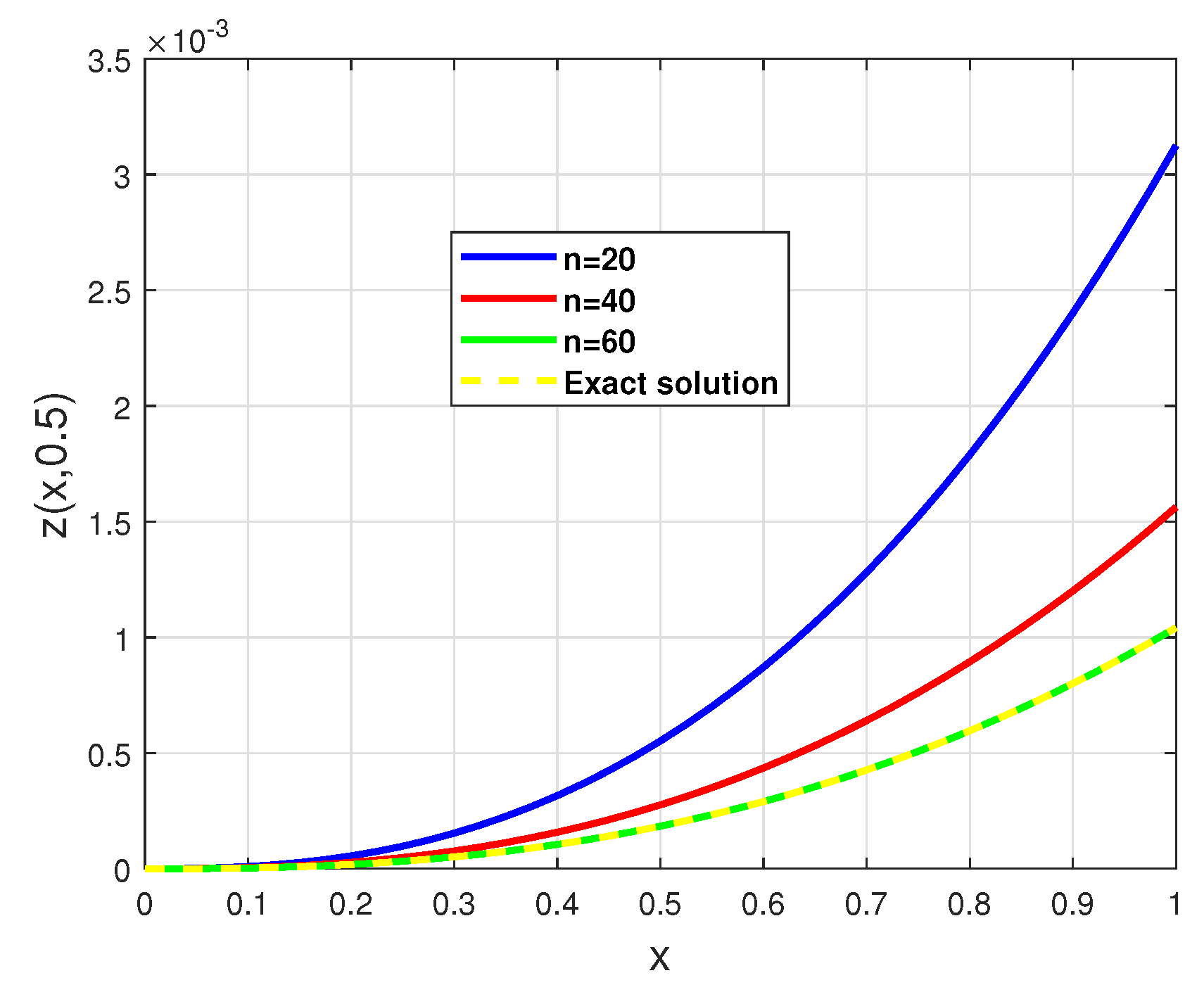
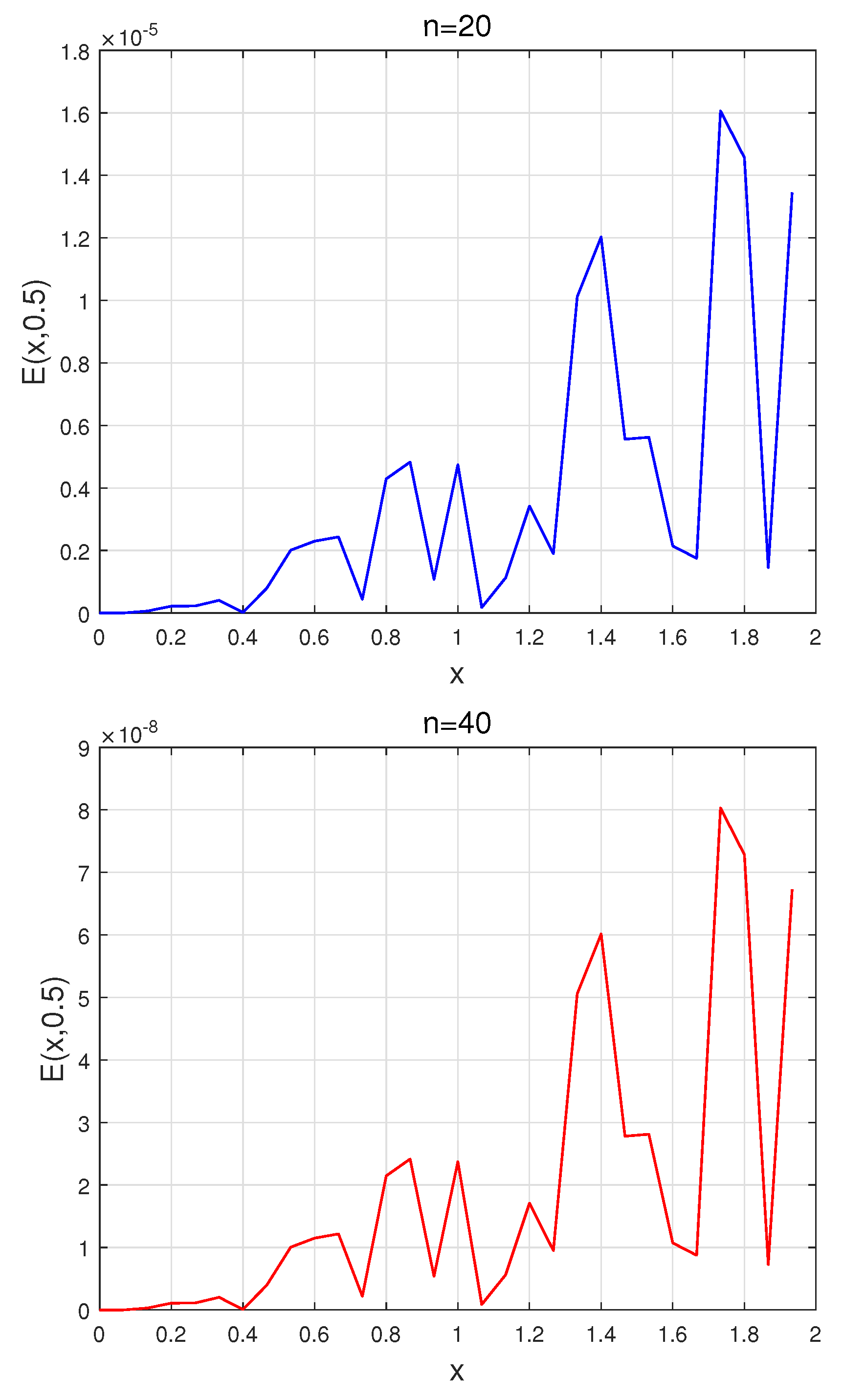
4. Illustrative Examples

This section presents numerical results computed for some examples, by applying the proposed method for a two-dimensional time-fractional ADE with distributed-order Riesz-space FDs. All calculations were carried out with the software package MATLAB 2016b on a PC with 8 GB of RAM. We illustrate the accuracy of the new method by computing the maximum absolute error E ( x , t ) :
E ( x , t ) = max | z ( x l , t j ) z n | ,
where z ( x , t ) and z n denote the exact and approximate solutions, respectively.
Example 1.
We address the time-fractional and distributed-order Riesz-space fractional ADE:
C D t α z ( x , t ) = 1 2 κ ( p ) p z ( x , t ) x p d p + 1 2 κ ( q ) q z ( x , t ) x q d q + + z ( x , t ) + f ( x , t ) ,
under the IBCs
z ( 0 , t ) = 0 , z ( 1 , t ) = t 2 ( 1 t ) 2 , z ( x , 0 ) = 0 ,
in which κ ( p ) = 8 Γ ( 7 2 p ) cos ( p π 2 ) 15 π , κ ( q ) = 8 Γ ( 7 2 q ) cos ( q π 2 ) 15 π and
f ( x , t ) = 2 Γ ( 3 α ) t 2 α + 24 Γ ( 5 α ) t 4 α 12 Γ ( 4 α ) t 3 α x 5 2 + 2 t 2 ( 1 t ) 2 1 x ln ( 1 x ) + x x 1 ln ( x ) x 5 2 t 2 ( 1 t ) 2 .
The exact solution for this Example 1 is z ( x , t ) = x 5 2 t 2 ( 1 t ) 2 . Figure 1 depicts the solution for Example 1 using the proposed method on the interval [ 0 , 1 ] × [ 0 , 1 ] with various choices of n for α = 0.75 and T = T = 10 . Figure 2 compares the exact and numerical solutions at t = 0.5 . Figure 3 illustrates the absolute error for different choices of n for α = 0.75 with T = T = 10 . Figure 4 depicts the absolute error at t = 0.5 . In Table 1, we compare the exact and numerical solutions at t = 0.5 for different values of n for α = 0.75 with T = T = 10 .
Example 2.
We solve the time-fractional ADE with distributed-order Riesz-space FDs:
C D t α z ( x , t ) = 1 2 κ ( p ) p z ( x , t ) x p d p + 1 2 κ ( q ) q z ( x , t ) x q d q + + z 2 ( x , t ) + f ( x , t ) ,
under the IBCs
z ( 0 , t ) = 0 , z ( 2 , t ) = 4 t ( t 2 ) , z ( x , 0 ) = 0 ,
in which κ ( p ) = Γ ( 3 p ) cos ( p π 2 ) , κ ( q ) = Γ ( 3 q ) cos ( q π 2 ) and
f ( x , t ) = 2 Γ ( 3 α ) t 2 α 2 Γ ( 2 α ) t 1 α x 2 + 2 t ( t 2 ) 1 x ln ( 2 x ) + x 1 ln ( x ) x 4 t ( t 2 ) 2 .
The exact solution for this Example 2 is z ( x , t ) = x 2 t ( t 2 ) . Figure 5 shows the approximate solution for different values of n for α = 0.75 with T = T = 10 . Figure 6 compares the exact and numerical solutions at t = 0.5 . Figure 7 illustrates the absolute error for different values of n for α = 0.75 with T = T = 10 . Figure 8 depicts the absolute error at t = 0.5 . In Table 2, we compare the exact and numerical solutions at t = 0.5 for different values of n for α = 0.75 with T = T = 10 .

5. Conclusions

We investigated and validated the numerical solution of the nonlinear time-fractional ADE with distributed-order Riesz-space FDs under IBCs. We employed two numerical approaches to estimate the proposed equation. For approximating the Riesz FD in space, we employed the finite difference approach based on the matrix transform algorithm, and for estimating the time-fractional ADE, we used the compound Simpson method. The stability and convergence of the proposed method were theoretically proven. Finally, some numerical experiments were performed to demonstrate and validate the accuracy of the new technique. In future work, numerical schemes based on alternating direction implicit methods for the two-dimensional nonlinear time-fractional ADE with distributed-order Riesz-space FDs under the IBCs will be investigated, and a high-order method for the two-dimensional nonlinear time-fractional ADE will be presented.

Author Contributions

Investigation, methodology and writing—original draft, M.D., A.S.H. and M.A.Z.; software and conceptualization, M.D.; writing—review and editing, A.S.H., A.M.L., A.G. and M.A.Z.; visualization and supervision, A.S.H., A.M.L., A.G. and M.A.Z. All authors have read and agreed to the published version of the manuscript.

Funding

This work was supported and funded by the Deanship of Scientific Research at Imam Mohammad Ibn Saud Islamic University (IMSIU) (grant number IMSIU-RP23095).

Data Availability Statement

Raw data were generated at Zand Institute of Higher Education, Faculty of Technology and Engineering, Shiraz, Iran. Derived data supporting the findings of this study are available from the author Mohammadhossein Derakhshan on request.

Acknowledgments

The authors gratefully acknowledge the technical and financial support provided by the Deanship of Scientific Research at Imam Mohammad Ibn Saud Islamic University (IMSIU).

Conflicts of Interest

The authors declare no conflict of interest.

References

  1. Podulbny, I. Fractional Differential Equations; Academic Press: New York, NY, USA, 1999. [Google Scholar]
  2. Kilbas, A.A.; Srivastava, H.M.; Trujillo, J.J. Theory and Applications of Fractional Differential Equations; Elsevier: Amsterdam, The Netherlands, 2006; Volume 204. [Google Scholar]
  3. Mainardi, F.; Pagnini, G.; Gorenflo, R. Some aspects of fractional diffusion equations of single and distributed order. Appl. Math. Comput. 2007, 187, 295–305. [Google Scholar] [CrossRef]
  4. Derakhshan, M.; Aminataei, A. New approach for the chaotic dynamical systems involving Caputo-Prabhakar fractional derivative using Adams-Bashforth scheme. J. Differ. Equ. Appl. 2021, 1–17. [Google Scholar] [CrossRef]
  5. Ata, E.; Kıymaz, I.O. New generalized Mellin transform and applications to partial and fractional differential equations. Int. J. Math. Comput. Eng. 2023, 1, 45–66. [Google Scholar] [CrossRef]
  6. Jafari, H.; Goswami, P.; Dubey, R.; Sharma, S.; Chaudhary, A. Fractional SZIR Model of Zombies Infection. Authorea 2022. [Google Scholar] [CrossRef]
  7. Singh, R.; Mishra, J.; Gupta, V.K. The dynamical analysis of a Tumor Growth model under the effect of fractal fractional Caputo-Fabrizio derivative. Int. J. Math. Comput. Eng. 2023, 1, 115–126. [Google Scholar] [CrossRef]
  8. Qin, S.; Liu, F.; Turner, I.; Vegh, V.; Yu, Q.; Yang, Q. Multi-term time-fractional Bloch equations and application in magnetic resonance imaging. J. Comput. Appl. Math. 2017, 319, 308–319. [Google Scholar] [CrossRef]
  9. Srivastava, V.; Rai, K. A multi-term fractional diffusion equation for oxygen delivery through a capillary to tissues. Math. Comput. Model. 2010, 51, 616–624. [Google Scholar] [CrossRef]
  10. Huang, J.; Zhang, J.; Arshad, S.; Tang, Y. A numerical method for two-dimensional multi-term time-space fractional nonlinear diffusion-wave equations. Appl. Numer. Math. 2021, 159, 159–173. [Google Scholar] [CrossRef]
  11. Lorenzo, C.F.; Hartley, T.T. Variable order and distributed order fractional operators. Nonlinear Dyn. 2002, 29, 57–98. [Google Scholar] [CrossRef]
  12. Atanackovic, T. A generalized model for the uniaxial isothermal deformation of a viscoelastic body. Acta Mech. 2002, 159, 77–86. [Google Scholar] [CrossRef]
  13. Zaky, M.A.; Machado, J.T. On the formulation and numerical simulation of distributed-order fractional optimal control problems. Commun. Nonlinear Sci. Numer. Simul. 2017, 52, 177–189. [Google Scholar] [CrossRef]
  14. Yuttanan, B.; Razzaghi, M. Legendre wavelets approach for numerical solutions of distributed order fractional differential equations. Appl. Math. Model. 2019, 70, 350–364. [Google Scholar] [CrossRef]
  15. Fardi, M.; Zaky, M.; Hendy, A. Nonuniform difference schemes for multi-term and distributed-order fractional parabolic equations with fractional Laplacian. Math. Comput. Simul. 2023, 206, 614–635. [Google Scholar] [CrossRef]
  16. Diethelm, K.; Ford, N.J. Numerical analysis for distributed-order differential equations. J. Comput. Appl. Math. 2009, 225, 96–104. [Google Scholar] [CrossRef]
  17. Ford, N.J.; Luisa Morgado, M.; Rebelo, M. An implicit finite difference approximation for the solution of the diffusion equation with distributed order in time. Electron. Trans. Numer. Anal. 2015, 44, 289–305. [Google Scholar]
  18. Ye, H.; Liu, F.; Anh, V.; Turner, I. Numerical analysis for the time distributed-order and Riesz space fractional diffusions on bounded domains. IMA J. Appl. Math. 2015, 80, 825–838. [Google Scholar] [CrossRef]
  19. Yang, X.; Zhang, H.; Xu, D. WSGD-OSC scheme for two-dimensional distributed order fractional reaction–diffusion equation. J. Sci. Comput. 2018, 76, 1502–1520. [Google Scholar] [CrossRef]
  20. Hu, X.; Liu, F.; Turner, I.; Anh, V. An implicit numerical method of a new time distributed-order and two-sided space-fractional advection-dispersion equation. Numer. Algorithms 2016, 72, 393–407. [Google Scholar] [CrossRef]
  21. Zaky, M.A.; Machado, J.T. Multi-dimensional spectral tau methods for distributed-order fractional diffusion equations. Comput. Math. Appl. 2020, 79, 476–488. [Google Scholar] [CrossRef]
  22. Shi, Y.; Liu, F.; Zhao, Y.; Wang, F.; Turner, I. An unstructured mesh finite element method for solving the multi-term time fractional and Riesz space distributed-order wave equation on an irregular convex domain. Appl. Math. Model. 2019, 73, 615–636. [Google Scholar] [CrossRef]
  23. Moghaddam, B.; Machado, J.T.; Morgado, M. Numerical approach for a class of distributed order time fractional partial differential equations. Appl. Numer. Math. 2019, 136, 152–162. [Google Scholar] [CrossRef]
  24. Chen, H.; Lü, S.; Chen, W. Finite difference/spectral approximations for the distributed order time fractional reaction–diffusion equation on an unbounded domain. J. Comput. Phys. 2016, 315, 84–97. [Google Scholar] [CrossRef]
  25. Morgado, M.L.; Rebelo, M.; Ferras, L.L.; Ford, N.J. Numerical solution for diffusion equations with distributed order in time using a Chebyshev collocation method. Appl. Numer. Math. 2017, 114, 108–123. [Google Scholar] [CrossRef]
  26. Zaky, M.; Doha, E.; Tenreiro Machado, J. A spectral numerical method for solving distributed-order fractional initial value problems. J. Comput. Nonlinear Dyn. 2018, 13, 101007. [Google Scholar] [CrossRef]
  27. Fei, M.; Huang, C. Galerkin–Legendre spectral method for the distributed-order time fractional fourth-order partial differential equation. Int. J. Comput. Math. 2020, 97, 1183–1196. [Google Scholar] [CrossRef]
  28. Ilic, M.; Liu, F.; Turner, I.; Anh, V. Numerical approximation of a fractional-in-space diffusion equation (II)–with nonhomogeneous boundary conditions. Fract. Calc. Appl. Anal. 2006, 9, 333–349. [Google Scholar]
  29. Zhang, H.; Liu, F.; Jiang, X.; Zeng, F.; Turner, I. A Crank–Nicolson ADI Galerkin–Legendre spectral method for the two-dimensional Riesz space distributed-order advection–diffusion equation. Comput. Math. Appl. 2018, 76, 2460–2476. [Google Scholar] [CrossRef]
  30. Ansari, A.; Derakhshan, M.H. On spectral polar fractional Laplacian. Math. Comput. Simul. 2023, 206, 636–663. [Google Scholar] [CrossRef]
  31. Li, C.; Zeng, F. Numerical Methods for Fractional Calculus; CRC Press: Boca Raton, FL, USA, 2015; Volume 24. [Google Scholar]
  32. Salkuyeh, D.K. On the finite difference approximation to the convection–diffusion equation. Appl. Math. Comput. 2006, 179, 79–86. [Google Scholar] [CrossRef]
Figure 1. Solution for Example 1 with different values of n for α = 0.75 with T = T = 10 .
Fractalfract 07 00649 g001aFractalfract 07 00649 g001b
Figure 2. Numerical and exact solutions for Example 1 with different values of n for α = 0.75 with T = T = 10 , at t = 0.5 .
Fractalfract 07 00649 g002
Figure 3. Absolute errors with various values of n for α = 0.75 with T = T = 10 for Example 1.
Fractalfract 07 00649 g003
Figure 4. Absolute errors with various values of n for α = 0.75 with T = T = 10 , at t = 0.5 for Example 1.
Fractalfract 07 00649 g004
Figure 5. Approximations for Example 2 with different values of n for α = 0.75 with T = T = 10 .
Fractalfract 07 00649 g005
Figure 6. Approximate and exact solutions for Example 2 with different values of n for α = 0.75 with T = T = 10 , at t = 0.5 .
Fractalfract 07 00649 g006
Figure 7. Absolute errors for Example 2 with different values of n for α = 0.75 with T = T = 10 .
Fractalfract 07 00649 g007aFractalfract 07 00649 g007b
Figure 8. Absolute errors for Example 2 with different values of n for α = 0.75 with T = T = 10 , at t = 0.5 .
Fractalfract 07 00649 g008aFractalfract 07 00649 g008b
Table 1. The absolute errors with various values of n for α = 0.75 with T = T = 10 for Example 1.
E ( x , t )
( x , t ) n = 20 n = 40 n = 60
( 0.1 , 0.1 ) 7.7495 × 10 10 7.9413 × 10 18 8.2919 × 10 30
( 0.2 , 0.2 ) 3.3200 × 10 10 3.3419 × 10 18 3.3898 × 10 30
( 0.3 , 0.3 ) 5.4883 × 10 10 5.3308 × 10 18 5.4776 × 10 30
( 0.4 , 0.4 ) 8.2341 × 10 10 8.3890 × 10 18 8.4384 × 10 30
( 0.5 , 0.5 ) 6.6285 × 10 10 5.7829 × 10 18 5.7829 × 10 30
( 0.6 , 0.6 ) 5.2021 × 10 10 4.9610 × 10 18 5.1242 × 10 30
( 0.7 , 0.7 ) 9.4310 × 10 10 8.9003 × 10 18 7.2027 × 10 30
( 0.8 , 0.8 ) 4.4560 × 10 10 2.2477 × 10 18 6.6203 × 10 31
( 0.9 , 0.9 ) 9.3799 × 10 10 9.0139 × 10 18 7.0545 × 10 30
C O 1.61 1.65 1.11
C P U t i m e ( s ) 57.56 252.75 5458.33
Table 2. The absolute errors for various values of n for α = 0.75 with T = T = 10 for Example 2.
E ( x , t )
( x , t ) n = 20 n = 40 n = 60
( 0.1 , 0.2 ) 1.1668 × 10 11 5.8340 × 10 14 3.8893 × 10 16
( 0.2 , 0.4 ) 2.0264 × 10 11 1.0132 × 10 13 6.7547 × 10 16
( 0.3 , 0.6 ) 2.4493 × 10 10 1.2247 × 10 12 8.1645 × 10 15
( 0.4 , 0.8 ) 8.7688 × 10 11 4.3844 × 10 13 2.9229 × 10 15
( 0.5 , 1 ) 1.0531 × 10 09 5.2657 × 10 12 3.5105 × 10 14
( 0.6 , 1.2 ) 9.8788 × 10 10 4.9394 × 10 12 3.2929 × 10 14
( 0.7 , 1.4 ) 6.0759 × 10 10 3.0380 × 10 12 2.0253 × 10 14
( 0.8 , 1.6 ) 3.9332 × 10 09 1.9666 × 10 11 1.3111 × 10 13
( 0.9 , 1.8 ) 6.7664 × 10 10 3.3832 × 10 12 2.2555 × 10 14
C O 1.044 0.997 0.989
C P U t i m e ( s ) 3878159
Disclaimer/Publisher’s Note: The statements, opinions and data contained in all publications are solely those of the individual author(s) and contributor(s) and not of MDPI and/or the editor(s). MDPI and/or the editor(s) disclaim responsibility for any injury to people or property resulting from any ideas, methods, instructions or products referred to in the content.

