Approximate Analytical Solution of Fuzzy Linear Volterra Integral Equation via Elzaki ADM

Abstract

In this paper, the fuzzy Volterra integral equations’ solutions are calculated using a hybrid methodology. The combination of the Elzaki transform and Adomian decomposition method results in the development of a novel regime. The precise fuzzy solutions are determined using Elzaki ADM after the fuzzy linear Volterra integral equations are first translated into two crisp integral equations utilizing the fuzzy number in parametric form. Three instances of the considered equations are solved to show the established scheme’s dependability, efficacy, and application. The results have a substantial impact on the fuzzy analytical dynamic equation theory. The comparison of the data in a graphical and tabular format demonstrates the robustness of the defined regime. The lower and upper bound solutions’ theoretical convergence and error estimates are highlighted in this paper. A tolerable order of absolute error is also obtained for this inquiry, and the consistency of the outcomes that are approximated and accurate is examined. The regime generated effective and reliable results. The current regime effectively lowers the computational cost, and a faster convergence of the series solution to the exact answer is signaled.

1. Introduction

One of the most often utilized fields of mathematics is fuzzy fractional calculus theory, which has both theoretical and practical applications embracing a wide range of mathematical structures. Traditional derivatives mostly rely on Caputo–Liouville or Riemann–Liouville concerns in this market segment. The nonlocality and singularity of the kernel function, which is visible in the integral operator’s side-by-side with the normalizing function showing alongside the integral ticks, are the most common defects of these two qualifiers. A more accurate and precise characterization must unavoidably follow from the reality of core replicating dynamic fractional systems. The Atangana–Baleanu Caputo is a novel fractional fuzzy derivative construct introduced in this orientation, which is utilized to synthesize and explicate fresh fuzzy real-world mathematical concepts.

The fuzzy set theory is useful for analyzing ambiguous situations. Any element of a fractional equation, including the initial value and boundary conditions, may be impacted by these uncertainties. The recognition of fractional models in practical contexts leads to the usage of interval or fuzzy formulations as an alternative. Numerous fields, including topology, fixed-point theory, integral inequalities, fractional calculus, bifurcation, image processing, consumer electronics, control theory, artificial intelligence, and operations research, have made extensive use of the fuzzy set theory. Over the past few decades, the field of fractional calculus, which encompasses fractional-order integrals and derivatives, has attracted a great lot of attention from academics and scientists. Because it yields precise and accurate conclusions, fractional calculus has a wide range of applications in contemporary physical and biological processes. The integral (differential) operators have more latitude in fractional differential calculus. As a result, academics are quite interested in this subject. Over the past few decades, a large number of research papers, monographs, and books on a variety of themes, including existence theory and analytical conclusions, have been published.

The study of fuzzy integral equations is rapidly spreading and expanding, especially in light of its recently recognized relationship to fuzzy control. Understanding integral equations is important since they serve as the foundation for the bulk of mathematical models applied to problems in a variety of fields, including chemistry, engineering, biology, and physics. Mathematicians regularly use differential, fractional order differential, and integral equations to resolve problems in the fields of chemistry, engineering, biology, physics, and other sciences. Undoubtedly, any model has some parameters that might be transmitted with some ambiguity. These ambiguous research problems, which result in the presentation of fuzzy conceptions, are necessary to solve these models. Richening fuzzy equation answers have received a lot of attention in the literature.

Fuzzy Sumudu transform technology was offered by Khan et al. [1] for the resolution of fuzzy differential equations. Homotopy analysis was provided by Maitama and Zhou [2]. Fuzzy differential equations having derivatives of both fractional and integer orders can be handled using the Shehu transform approach. Results on nth-order fuzzy differential equations with GH-differentiability were reported by Khastan et al. in their paper published in 2008 [3]. Applications of the fuzzy Laplace transform were provided by Salahshour and Allahviranloo [4]. A unique method for solving fuzzy linear differential equations was presented by Allahviranloo et al. [5]. Laplace transform was used by Salgado et al. [6] to find solutions for interactive fuzzy equations. Laplace ADM was used by Ullah et al. [7] to propose a solution to fuzzy Volterra integral equations. Applications of the double Sumudu ADM for 2D fuzzy Volterra integral equations were announced by Alidema [8].

The classical Volterra integral equation is given by

$$\theta \left(y\right)=h\left(y\right)+{\lambda }_1{\int }_{{\beta }_1}^{y}k\left(y,s\right)\theta \left(s\right)ds.$$

(1)

The fuzzy form of the differential equation is given as follows:

$$\theta \left(y,{\alpha }_1\right)=h\left(y,{\alpha }_1\right)+{\lambda }_1{\int }_{{\beta }_1}^{y}k\left(y,s\right)\theta \left(s,{\alpha }_1\right)ds.$$

(2)

where the unknown fuzzy parameter function is as follows:

$$\theta \left(y,{\alpha }_1\right)=\left[\underset{\_}{\theta }\left(y,{\alpha }_1\right),\stackrel{\_}{\theta }\left(y,{\alpha }_1\right)\right].$$

and is to be evaluated.

$$h\left(y,{\alpha }_1\right)=\left[\underset{\_}{h}\left(y,{\alpha }_1\right),\stackrel{\_}{h}\left(y,{\alpha }_1\right)\right].$$

is considered as the fuzzy parametric form function and $k\left(y,s\right)$ is a real valued function which is also considered as the kernel of the integral equation.

2. Preliminaries

Definition 1. [6].

Let $\varphi :R\to E$ is a fuzzy valued function s.t. $r\in \left[\mathrm{0,1}\right]$

$${\left[\varphi \left(x\right)\right]}^r=\left[\underset{\_}{{\varphi }_r\left(x\right)},\stackrel{\_}{{\varphi }_r\left(x\right)}\right].$$

1.

If $\varphi \left(x\right)$ is a differentiable function in first form i.e., (1) differentiable, then

$${\left[{\varphi }^{\prime }\left(x\right)\right]}^r=\left[\underset{\_}{{\varphi }_r\prime \left(x\right)},\stackrel{\_}{{\varphi }_r^{\prime }\left(x\right)}\right].$$

2.

If $\varphi \left(x\right)$ is a differentiable function in second form i.e., (2) differentiable, then

$${\left[{\varphi }^{\prime }\left(x\right)\right]}^r=\left[\stackrel{\_}{{\varphi }_r^{\prime }\left(x\right)},\underset{\_}{{\varphi }_r\prime \left(x\right)}\right].$$

Definition 2.

Let $\varphi :\left(a,b\right)\to E$ is strongly generalized H-differentiable function at $x_0\in \left(a,b\right)$ if there exists ${\varphi }^{\prime }\left(x_0\right)\in E$ s.t. for $h>0$ and closed to zero.

1.

${\varphi }^{\prime }\left(x_0\right)=\underset{h\to 0}{\lim }\frac{\varphi \left(x_0+h\right)\mathsf{\Theta }\varphi \left(x_0\right)}{h}=\underset{h\to 0}{\lim }\frac{\varphi \left(x_0\right)\mathsf{\Theta }\varphi \left(x_0-h\right)}{h}.$

2.

${\varphi }^{\prime }\left(x_0\right)=\underset{h\to 0}{\lim }\frac{\varphi \left(x_0\right)\mathsf{\Theta }\varphi \left(x_0+h\right)}{-h}=\underset{h\to 0}{\lim }\frac{\varphi \left(x_0-h\right)\mathsf{\Theta }\varphi \left(x_0\right)}{-h}.$

3.

${\varphi }^{\prime }\left(x_0\right)=\underset{h\to 0}{\lim }\frac{\varphi \left(x_0+h\right)\mathsf{\Theta }\varphi \left(x_0\right)}{h}=\underset{h\to 0}{\lim }\frac{\varphi \left(x_0-h\right)\mathsf{\Theta }\varphi \left(x_0\right)}{-h}.$

4.

${\varphi }^{\prime }\left(x_0\right)=\underset{h\to 0}{\lim }\frac{\varphi \left(x_0\right)\mathsf{\Theta }\varphi \left(x_0+h\right)}{-h}=\underset{h\to 0}{\lim }\frac{\varphi \left(x_0\right)\mathsf{\Theta }\varphi \left(x_0-h\right)}{h}.$

Definition 3.

Considereing that $\varphi \left(x\right),{\varphi }^{\prime }\left(x\right),\dots ,{\varphi }^{\left(n-1\right)}\left(x\right)$ are differentiable fuzzy valued functions with r-cut form

$${\left[\varphi \left(x\right)\right]}^r=\left[\underset{\_}{{\varphi }_r\left(x\right)},\stackrel{\_}{{\varphi }_r\left(x\right)}\right].$$

1.

If $\varphi \left(x\right),{\varphi }^{\prime }\left(x\right),\dots ,{\varphi }^{\left(n-1\right)}\left(x\right)$ are (1) differentiable

$${\left[{\varphi }^n\left(x\right)\right]}^r=\left[\underset{\_}{{\varphi }_r^{\left(n\right)}\left(x\right)},\stackrel{\_}{{\varphi }_r^{\left(n\right)}\left(x\right)}\right].$$

2.

If $\varphi \left(x\right),{\varphi }^{\prime }\left(x\right),\dots ,{\varphi }^{\left(n-1\right)}\left(x\right)$ are (2) differentiable

$${\left[{\varphi }^n\left(x\right)\right]}^r=\left[\underset{\_}{{\varphi }_r^{\left(n\right)}\left(x\right)},\stackrel{\_}{{\varphi }_r^{\left(n\right)}\left(x\right)}\right].$$

3.

If $\varphi \left(x\right)$ is (1)-differentiable and ${\varphi }^{\prime }\left(x\right),\dots ,{\varphi }^{\left(n-1\right)}\left(x\right)$ are (2) differentiable

$${\left[{\varphi }^n\left(x\right)\right]}^r=\left[\stackrel{\_}{{\varphi }_r^{\left(n\right)}\left(x\right)},\underset{\_}{{\varphi }_r^{\left(n\right)}\left(x\right)}\right].$$

4.

If $\varphi \left(x\right)$ is (2)-differentiable and ${\varphi }^{\prime }\left(x\right),\dots ,{\varphi }^{\left(n-1\right)}\left(x\right)$ are (1) differentiable

$${\left[{\varphi }^n\left(x\right)\right]}^r=\left[\stackrel{\_}{{\varphi }_r^{\left(n\right)}\left(x\right)},\underset{\_}{{\varphi }_r^{\left(n\right)}\left(x\right)}\right].$$

Definition 4.

Elzaki transform is defined as follows:

$$E\left(\nu \right)=\nu {\int }_0^{\infty }f\left(t\right)e^{-\left(\frac{t}{\nu }\right)}dt.$$

(3)

where $f\left(t\right)$ is considered as the time function.

$$E\left[u_t\left(x,t\right)\right]=\frac{1}{\nu }E\left[u\left(x,t\right)\right]-\nu u\left(x,0\right),$$

(4)

$$E\left[u_t\left(x,y,t\right)\right]=\frac{1}{\nu }E\left[u\left(x,y,t\right)\right]-\nu u\left(x,y,0\right),$$

(5)

$$E\left[u_t\left(x,y,z,t\right)\right]=\frac{1}{\nu }E\left[u\left(x,y,z,t\right)\right]-\nu u\left(x,y,z,0\right).$$

(6)

Via

Table 1. Elzaki transform of the given function.

$\mathit{f}\left(\mathit{t}\right)$	$\mathit{E}\left[\mathit{f}\right(\mathit{t}\left)\right]=\mathit{T}\left(\mathit{\nu }\right)$
$1$	${\nu }^2$
$t$	${\nu }^3$
$t^n$	$\angle n{\nu }^{n+2}$
$e^{at}$	$\frac{{\nu }^2}{1-a\nu }$
$\sin \left(at\right)$	$\frac{a{\nu }^3}{1+a^2{\nu }^2}$
$\cos \left(at\right)$	$\frac{a{\nu }^2}{1+a^2{\nu }^2}$
$\sinh \left(at\right)$	$\frac{a{\nu }^3}{1-a^2{\nu }^2}$
$\cosh \left(at\right)$	$\frac{a{\nu }^2}{1-a^2{\nu }^2}$

, the basic properties of the Elzaki transform are mentioned.

ADM’s key benefit is that it does not rely on perturbation, linearization, or any other kind of discretization. The actual result of the model thus stays the same. It is not necessary to discretize the variables, which is a complex and challenging approach. This indicates that the results were produced without any errors, which was made possible by discretization. It is also precise in determining the approximate and exact solutions of nonlinear prototypes. Different types of differential equations, including integro-differential equations, differential algebraic equations, and differential-difference equations, as well as some functional equations, eigenvalue problems, and stochastic system problems, can all be solved using such techniques. Some of the latest references regarding the solution of different differential equations are as follows [9,10,11,12,13,14,15,16].

3. The Main Advantages of the Study

The fuzzy Volterra Integral equation is solved in current research using an iterative regime devised and included under the name Elzaki ADM. Numerical discretization under the current regime does not require any complicated calculations and is simple to implement. To obtain the approximated-analytical solutions, innovative iterative regimes must be created because it is difficult to create numerical programs to handle fractional PDEs. There are many transforms described in the literature, but depending on how they affect calculations, some transforms are simple to use, and others are not. One of the simplest techniques is the Elzaki ADM. It has been observed through a review of the literature that fuzzy Volterra Integral equations are rarely resolved. As a result, the originality of the research lies in its focus on identifying a solution to the problem. This article also elaborates on error analysis and convergence analysis.

4. Basic Notion of Regime

The parametric form of the considered equation is as follows:

$$\left\{\begin{array}{c}\underset{\_}{\theta }\left(y,{\alpha }_1\right)=\underset{\_}{h}\left(y,{\alpha }_1\right)+{\int }_{{\beta }_1}^{y}k\left(y,s\right)\underset{\_}{\theta }\left(s,{\alpha }_1\right)ds,\\ \stackrel{\_}{\theta }\left(y,{\alpha }_1\right)=\stackrel{\_}{h}\left(y,{\alpha }_1\right)+{\int }_{{\beta }_1}^{y}k\left(y,s\right)\stackrel{\_}{\theta }\left(s,{\alpha }_1\right)ds.\end{array}\right.$$

Applying Elzaki transform:

$$\left\{\begin{array}{c}E\left[\underset{\_}{\theta }\left(y,{\alpha }_1\right)\right]=E\left[\underset{\_}{h}\left(y,{\alpha }_1\right)\right]+E\left[{\int }_{{\beta }_1}^{y}k\left(y,s\right)\underset{\_}{\theta }\left(s,{\alpha }_1\right)ds\right],\\ E\left[\stackrel{\_}{\theta }\left(y,{\alpha }_1\right)\right]=E\left[\stackrel{\_}{h}\left(y,{\alpha }_1\right)\right]+E\left[{\int }_{{\beta }_1}^{y}k\left(y,s\right)\stackrel{\_}{\theta }\left(s,{\alpha }_1\right)ds\right].\end{array}\right.$$

By the notion of the Convolution theorem for the Elzaki transform:

$$\left\{\begin{array}{c}E\left[\underset{\_}{\theta }\left(y,{\alpha }_1\right)\right]=E\left[\underset{\_}{h}\left(y,{\alpha }_1\right)\right]+\frac{1}{u}E\left[y\right]E\left[\underset{\_}{\theta }\left(y,{\alpha }_1\right)\right],\\ E\left[\stackrel{\_}{\theta }\left(y,{\alpha }_1\right)\right]=E\left[\stackrel{\_}{h}\left(y,{\alpha }_1\right)\right]+\frac{1}{u}E\left[y\right]E\left[\stackrel{\_}{\theta }\left(y,{\alpha }_1\right)\right].\end{array}\right.$$

$$\left\{\begin{array}{c}E\left[\underset{\_}{\theta }\left(y,{\alpha }_1\right)\right]=E\left[\underset{\_}{h}\left(y,{\alpha }_1\right)\right]+u^{2}E\left[\underset{\_}{\theta }\left(y,{\alpha }_1\right)\right],\\ E\left[\stackrel{\_}{\theta }\left(y,{\alpha }_1\right)\right]=E\left[\stackrel{\_}{h}\left(y,{\alpha }_1\right)\right]+u^{2}E\left[\stackrel{\_}{\theta }\left(y,{\alpha }_1\right)\right].\end{array}\right.$$

$$\left\{\begin{array}{c}\underset{\_}{\theta }\left(y,{\alpha }_1\right)=\underset{\_}{h}\left(y,{\alpha }_1\right)+E^{-1}\left[u^{2}E\left[\underset{\_}{\theta }\left(y,{\alpha }_1\right)\right]\right],\\ \stackrel{\_}{\theta }\left(y,{\alpha }_1\right)=\stackrel{\_}{h}\left(y,{\alpha }_1\right)+E^{-1}\left[u^{2}E\left[\stackrel{\_}{\theta }\left(y,{\alpha }_1\right)\right]\right].\end{array}\right.$$

Applying ADM:

$$\left\{\begin{array}{c}{\displaystyle \sum _{i=0}^{\infty }}\underset{\_}{{\theta }_i}\left(y,{\alpha }_1\right)=\underset{\_}{h}\left(y,{\alpha }_1\right)+E^{-1}\left[u^{2}E\left[{\displaystyle \sum _{i=0}^{\infty }}\underset{\_}{{\theta }_i}\left(y,{\alpha }_1\right)\right]\right],\\ {\displaystyle \sum _{i=0}^{\infty }}\stackrel{\_}{{\theta }_i}\left(y,{\alpha }_1\right)=\stackrel{\_}{h}\left(y,{\alpha }_1\right)+E^{-1}\left[u^{2}E\left[{\displaystyle \sum _{i=0}^{\infty }}\stackrel{\_}{{\theta }_i}\left(y,{\alpha }_1\right)\right]\right].\end{array}\right.$$

$$\left\{\begin{array}{c}\underset{\_}{{\theta }_0}\left(y,{\alpha }_1\right)+\underset{\_}{{\theta }_1}\left(y,{\alpha }_1\right)+\underset{\_}{{\theta }_2}\left(y,{\alpha }_1\right)+\underset{\_}{{\theta }_3}\left(y,{\alpha }_1\right)+\cdots \\ =\underset{\_}{h}\left(y,{\alpha }_1\right)+E^{-1}\left[u^{2}E\left[\underset{\_}{{\theta }_0}\left(y,{\alpha }_1\right)+\underset{\_}{{\theta }_1}\left(y,{\alpha }_1\right)+\underset{\_}{{\theta }_2}\left(y,{\alpha }_1\right)+\underset{\_}{{\theta }_3}\left(y,{\alpha }_1\right)+\cdots \right]\right]\\ \stackrel{\_}{{\theta }_0}\left(y,{\alpha }_1\right)+\stackrel{\_}{{\theta }_1}\left(y,{\alpha }_1\right)+\stackrel{\_}{{\theta }_2}\left(y,{\alpha }_1\right)+\stackrel{\_}{{\theta }_3}\left(y,{\alpha }_1\right)+\cdots \\ =\stackrel{\_}{h}\left(y,{\alpha }_1\right)+E^{-1}\left[u^{2}E\left[\stackrel{\_}{{\theta }_0}\left(y,{\alpha }_1\right)+\stackrel{\_}{{\theta }_1}\left(y,{\alpha }_1\right)+\stackrel{\_}{{\theta }_2}\left(y,{\alpha }_1\right)+\stackrel{\_}{{\theta }_3}\left(y,{\alpha }_1\right)+\cdots \right]\right].\end{array}\right.,$$

$$\left\{\begin{array}{c}\underset{\_}{{\theta }_0}\left(y,{\alpha }_1\right)=\underset{\_}{h}\left(y,{\alpha }_1\right),\\ \underset{\_}{{\theta }_1}\left(y,{\alpha }_1\right)=E^{-1}\left[u^{2}E\left[\underset{\_}{{\theta }_0}\left(y,{\alpha }_1\right)\right]\right],\\ \underset{\_}{{\theta }_2}\left(y,{\alpha }_1\right)=E^{-1}\left[u^{2}E\left[\underset{\_}{{\theta }_1}\left(y,{\alpha }_1\right)\right]\right],\\ \underset{\_}{{\theta }_3}\left(y,{\alpha }_1\right)=E^{-1}\left[u^{2}E\left[\underset{\_}{{\theta }_2}\left(y,{\alpha }_1\right)\right]\right],\\ ⋮\\ \underset{\_}{{\theta }_{n+1}}\left(y,{\alpha }_1\right)=S^{-1}\left[u^{2}E\left[\underset{\_}{{\theta }_n}\left(y,{\alpha }_1\right)\right]\right],n=0,1,2,3,\dots \end{array}\right.$$

$$\begin{array}{c}\stackrel{\_}{{\theta }_0}\left(y,{\alpha }_1\right)=\stackrel{\_}{h}\left(y,{\alpha }_1\right),\\ \stackrel{\_}{{\theta }_1}\left(y,{\alpha }_1\right)=S^{-1}\left[u^{2}E\left[\stackrel{\_}{{\theta }_0}\left(y,{\alpha }_1\right)\right]\right],\\ \stackrel{\_}{{\theta }_2}\left(y,{\alpha }_1\right)=S^{-1}\left[u^{2}E\left[\stackrel{\_}{{\theta }_1}\left(y,{\alpha }_1\right)\right]\right],\\ \stackrel{\_}{{\theta }_3}\left(y,{\alpha }_1\right)=S^{-1}\left[u^{2}E\left[\stackrel{\_}{{\theta }_2}\left(y,{\alpha }_1\right)\right]\right],\\ ⋮\\ \stackrel{\_}{{\theta }_{n+1}}\left(y,{\alpha }_1\right)=E^{-1}\left[u^{2}E\left[\stackrel{\_}{{\theta }_n}\left(y,{\alpha }_1\right)\right]\right],n=0,1,2,3,\dots \end{array}$$

5. Convergence Analysis and Error Estimate

Theorem 1.

(i) 

Let $X$ be a Banach space and let $\underset{\_}{{\theta }_m}(x,{\alpha }_1)$ and $\underset{\_}{{\theta }_n}(x,{\alpha }_1)$ be in $X$. Suppose $\gamma \in (0,1)$, then the series solution ${\left\{\underset{\_}{{\theta }_m}(x,{\alpha }_1)\right\}}_{m=0}^{\infty }$, which is defined, converges to the lower-bound solution whenever $\underset{\_}{{\theta }_m}\left(x,{\alpha }_1\right)\le \gamma \underset{\_}{{\theta }_{m-1}}(x,{\alpha }_1),\forall m>N$, that I,s for any given $\epsilon >0$, there exists a positive number $N$, such that $\left|\right|\underset{\_}{{\theta }_{m+n}}\left(x,{\alpha }_1\right)\left|\right|\le \mathit{ϵ},\forall m,n>N$.

(ii) 

Let ${\sum }_{i=0}^j\underset{\_}{{\theta }_i}\left(x,{\alpha }_1\right)$ be finite and $\underset{\_}{{\theta }_i}\left(x,{\alpha }_1\right)$ be its approximate solution. Suppose  $\gamma >0$, such that  $\left|\right|\underset{\_}{{\theta }_{i+1}}\left(x,{\alpha }_1\right)\left|\right|\le \gamma \left|\right|\underset{\_}{{\theta }_i}\left(x,{\alpha }_1\right)\left|\right|,\gamma \in \left(\mathrm{0,1}\right),\forall i$,  then the max. absolute error for the lower bound solution is: 

$$\left|\right|\underset{\_}{\theta }\left(x,{\alpha }_1\right)-\sum _{i=0}^j\underset{\_}{{\theta }_i}\left(x,{\alpha }_1\right)\left|\right|\le \frac{{\gamma }^{j+1}}{1-\gamma }\left|\right|\underset{\_}{{\theta }_0}\left(x,{\alpha }_1\right)\left|\right|$$

Proof. 

(i)

 

Provided $R_0\left(x,{\alpha }_1\right)=\underset{\_}{{\theta }_0}\left(x,{\alpha }_1\right),$

$$R_1\left(x,{\alpha }_1\right)=\underset{\_}{{\theta }_0}\left(x,{\alpha }_1\right)+\underset{\_}{{\theta }_1}\left(x,{\alpha }_1\right),$$

$$R_2\left(x,{\alpha }_1\right)=\underset{\_}{{\theta }_0}\left(x,{\alpha }_1\right)+\underset{\_}{{\theta }_1}\left(x,{\alpha }_1\right)+\underset{\_}{{\theta }_2}\left(x,{\alpha }_1\right),$$

$$R_3\left(x,{\alpha }_1\right)=\underset{\_}{{\theta }_0}\left(x,{\alpha }_1\right)+\underset{\_}{{\theta }_1}\left(x,{\alpha }_1\right)+\underset{\_}{{\theta }_2}\left(x,{\alpha }_1\right)+\underset{\_}{{\theta }_3}\left(x,{\alpha }_1\right),$$

$$\dots$$

$$R_m\left(x,{\alpha }_1\right)=\underset{\_}{{\theta }_0}\left(x,{\alpha }_1\right)+\underset{\_}{{\theta }_1}\left(x,{\alpha }_1\right)+\underset{\_}{{\theta }_2}\left(x,{\alpha }_1\right)+\underset{\_}{{\theta }_3}\left(x,{\alpha }_1\right)+\dots +\underset{\_}{{\theta }_m}(x,{\alpha }_1)$$

The aim is to prove that $R_m\left(x,{\alpha }_1\right)$ is a Cauchy sequence in the Banach space.

It is provided that for $\gamma \in \left(\mathrm{0,1}\right)$

$$\left|\left|R_{m+1}\left(x,{\alpha }_1\right)-R_m\left(x,{\alpha }_1\right)\right|\right|=\left|\right|\underset{\_}{{\theta }_{m+1}}\left(x,{\alpha }_1\right)\left|\right|$$

$$\le \gamma \left|\right|\underset{\_}{{\theta }_m}\left(x,{\alpha }_1\right)\left|\right|$$

$$\le {\gamma }^2\left|\right|\underset{\_}{{\theta }_{m-1}}\left(x,{\alpha }_1\right)\left|\right|$$

$$\le {\gamma }^3\left|\right|\underset{\_}{{\theta }_{m-2}}\left(x,{\alpha }_1\right)\left|\right|$$

$$\dots$$

$$\le {\gamma }^{m+1}\left|\right|\underset{\_}{{\theta }_0}\left(x,{\alpha }_1\right)\left|\right|.$$

Let find

$$\begin{gathered} \left|\right|R_m(x,{\alpha }_1)-R_n(x,{\alpha }_1)\left|\right| \\ =\left|\right|R_m\left(x,{\alpha }_1\right)-R_{m-1}\left(x,{\alpha }_1\right)+R_{m-1}\left(x,{\alpha }_1\right)-R_{m-2}\left(x,{\alpha }_1\right)+ \end{gathered}$$

$$R_{m-2}\left(x,{\alpha }_1\right)-R_{m-3}\left(x,{\alpha }_1\right)+\dots +R_{n+1}\left(x,{\alpha }_1\right)-R_n\left(x,{\alpha }_1\right)\left|\right|.$$

$$\begin{gathered} \left|\right|R_m(x,{\alpha }_1)-R_n(x,{\alpha }_1)\left|\right| \\ \le \left|\right|R_m\left(x,{\alpha }_1\right)-R_{m-1}\left(x,{\alpha }_1\right)\left|\right|+\left|\right|R_{m-1}\left(x,{\alpha }_1\right)-R_{m-2}\left(x,{\alpha }_1\right)\left|\right| \end{gathered}$$

$$+\left|\right|R_{m-2}\left(x,{\alpha }_1\right)-R_{m-3}\left(x,{\alpha }_1\right)\left|\right|+\dots +\left|\right|R_{n+1}\left(x,{\alpha }_1\right)-R_n\left(x,{\alpha }_1\right)\left|\right|.$$

$$\begin{gathered} \left|\right|R_m(x,{\alpha }_1)-R_n(x,{\alpha }_1)\left|\right| \\ ={\gamma }^m\left|\right|\underset{\_}{{\theta }_0}\left(x,{\alpha }_1\right)\left|\right| \\ +{\gamma }^{m-1}\left|\right|\underset{\_}{{\theta }_0}\left(x,{\alpha }_1\right)\left|\right|+{\gamma }^{m-2}\left|\right|\underset{\_}{{\theta }_0}\left(x,{\alpha }_1\right)\left|\right|+{\gamma }^{m-3}\left|\right|\underset{\_}{{\theta }_0}\left(x,{\alpha }_1\right)\left|\right|+\dots +{\gamma }^{n+1}\left|\right|\underset{\_}{{\theta }_0}\left(x,{\alpha }_1\right)\left|\right|. \end{gathered}$$

$$\left|\right|R_m\left(x,{\alpha }_1\right)-R_n\left(x,{\alpha }_1\right)\left|\right|\le \frac{(1-{\gamma }^{m-n})}{(1-\gamma )}{\gamma }^{n+1}\left|\right|\underset{\_}{{\theta }_0}\left(x,{\alpha }_1\right)\left|\right|.$$

Considering $ϵ=\frac{1-\gamma }{(1-{\gamma }^{m-n}){\gamma }^{n+1}\left|\right|\underset{\_}{{\theta }_0}\left(x,{\alpha }_1\right)\left|\right|}$

$$\left|\left|R_m\left(x,{\alpha }_1\right)-R_n\left(x,{\alpha }_1\right)\right|\right|<ϵ.$$

$$\underset{m,n\to \infty }{\lim }\left|\right|R_m\left(x,{\alpha }_1\right)-R_n\left(x,{\alpha }_1\right)\left|\right|=0.$$

$$\Rightarrow {\left\{R_m\right\}}_{m=0}^{\infty }\mathrm{is\; a\; Cauchy\; sequence}.$$

Let $\sum _{i=0}^j\underset{\_}{{\theta }_i}\left(x,{\alpha }_1\right)<\mathrm{\infty }$

$$\left|\right|\underset{\_}{\theta }\left(x,{\alpha }_1\right)-\sum _{i=0}^j\underset{\_}{{\theta }_i}\left(x,{\alpha }_1\right)\left|\right|=\left|\right|\sum _{i=j+1}^{\infty }\underset{\_}{{\theta }_i}\left(x,{\alpha }_1\right)\left|\right|$$

$$\le \sum _{i=j+1}^{\infty }\left|\right|\underset{\_}{{\theta }_i}\left(x,{\alpha }_1\right)\left|\right|$$

$$\le \sum _{i=j+1}^{\infty }{\gamma }^i\left|\right|\underset{\_}{{\theta }_0}\left(x,{\alpha }_1\right)\left|\right|$$

$$\le \left|\right|\underset{\_}{{\theta }_0}\left(x,{\alpha }_1\right)\left|\right|[{\gamma }^{j+1}+{\gamma }^{j+2}+{\gamma }^{j+3}+\cdots ].$$

$$\le \frac{\left|\right|\underset{\_}{{\theta }_0}\left(x,{\alpha }_1\right)\left|\right|{\gamma }^{j+1}}{1-\gamma }.\square$$

Theorem 2.

(i) 

Let $X$ be a Banach space and let $\stackrel{\_}{{\theta }_m}\left(x,{\alpha }_1\right)$ and $\stackrel{\_}{{\theta }_n}\left(x,{\alpha }_1\right)$ be in $X$. Suppose $\gamma \in (0,1)$, then the series solution ${\left\{\stackrel{\_}{{\theta }_m}\left(x,{\alpha }_1\right)\right\}}_{m=0}^{\infty }$, which is defined ${\sum }_{m=0}^{\infty }\stackrel{\_}{{\theta }_m}\left(x,{\alpha }_1\right)$, converges to the upper bound solution whenever $\stackrel{\_}{{\theta }_m}\left(x,{\alpha }_1\right)\le \gamma \stackrel{\_}{{\theta }_{m-1}}\left(x,{\alpha }_1\right),\forall m>N$, that is, for any given $\epsilon >0$, there exists a positive number $N$, such that $\left|\right|\stackrel{\_}{{\theta }_{m+n}}\left(x,{\alpha }_1\right)\left|\right|\le \mathit{ϵ},\forall m,n>N$.

(ii) 

Let  ${\sum }_{i=0}^j\stackrel{\_}{{\theta }_i}\left(x,{\alpha }_1\right)$  be finite and  $\stackrel{\_}{{\theta }_i}\left(x,{\alpha }_1\right)$  be its approximate solution. Suppose   $\gamma >0$, such that ||  $\stackrel{\_}{{\theta }_{i+1}}\left(x,{\alpha }_1\right)\left|\right|\le \gamma \left|\right|\stackrel{\_}{{\theta }_i}\left(x,{\alpha }_1\right)\left|\right|,\gamma \in \left(\mathrm{0,1}\right),\forall i$, then the max. absolute error for the upper bound solution is:

$$\left|\right|\underset{\_}{\theta }\left(x,{\alpha }_1\right)-\sum _{i=0}^j\stackrel{\_}{{\theta }_i}\left(x,{\alpha }_1\right)\left|\right|\le \frac{{\gamma }^{j+1}}{1-\gamma }\left|\right|\stackrel{\_}{{\theta }_0}\left(x,{\alpha }_1\right)\left|\right|.$$

Proof. 

(i)

 

Provided $S_0\left(x,{\alpha }_1\right)=\stackrel{\_}{{\theta }_0}\left(x,{\alpha }_1\right)$

$$S_1\left(x,{\alpha }_1\right)=\stackrel{\_}{{\theta }_0}\left(x,{\alpha }_1\right)+\stackrel{\_}{{\theta }_1}\left(x,{\alpha }_1\right),$$

$$S_2\left(x,{\alpha }_1\right)=\stackrel{\_}{{\theta }_0}\left(x,{\alpha }_1\right)+\stackrel{\_}{{\theta }_1}\left(x,{\alpha }_1\right)+\stackrel{\_}{{\theta }_2}\left(x,{\alpha }_1\right),$$

$$S_3\left(x,{\alpha }_1\right)=\stackrel{\_}{{\theta }_0}\left(x,{\alpha }_1\right)+\stackrel{\_}{{\theta }_1}\left(x,{\alpha }_1\right)+\stackrel{\_}{{\theta }_2}\left(x,{\alpha }_1\right)+\stackrel{\_}{{\theta }_3}\left(x,{\alpha }_1\right),$$

$$\dots$$

$$S_m\left(x,{\alpha }_1\right)=\stackrel{\_}{{\theta }_0}\left(x,{\alpha }_1\right)+\stackrel{\_}{{\theta }_1}\left(x,{\alpha }_1\right)+\stackrel{\_}{{\theta }_2}\left(x,{\alpha }_1\right)+\stackrel{\_}{{\theta }_3}\left(x,{\alpha }_1\right)$$

$$+\dots +\stackrel{\_}{{\theta }_m}\left(x,{\alpha }_1\right).$$

The aim is to prove that $S_m\left(x,{\alpha }_1\right)$ is a Cauchy sequence in the Banach space.

It is provided that for $\gamma \in \left(\mathrm{0,1}\right)$

$$\left|\left|S_{m+1}\left(x,{\alpha }_1\right)-S_m\left(x,{\alpha }_1\right)\right|\right|=\left|\right|\stackrel{\_}{{\theta }_{m+1}}\left(x,{\alpha }_1\right)\left|\right|$$

$$\le \gamma \left|\right|\stackrel{\_}{{\theta }_m}\left(x,{\alpha }_1\right)\left|\right|$$

$$\le {\gamma }^2\left|\right|\stackrel{\_}{{\theta }_{m-1}}\left(x,{\alpha }_1\right)\left|\right|$$

$$\le {\gamma }^3\left|\right|\stackrel{\_}{{\theta }_{m-2}}\left(x,{\alpha }_1\right)\left|\right|$$

$$\dots$$

$$\le {\gamma }^{m+1}\left|\right|\stackrel{\_}{{\theta }_0}\left(x,{\alpha }_1\right)\left|\right|.$$

Let find

$$\begin{gathered} \left|\right|S_m(x,{\alpha }_1)-S_n(x,{\alpha }_1)\left|\right| \\ =\left|\right|S_m\left(x,{\alpha }_1\right)-S_{m-1}\left(x,{\alpha }_1\right)+S_{m-1}\left(x,{\alpha }_1\right)-S_{m-2}\left(x,{\alpha }_1\right)+ \end{gathered}$$

$$S_{m-2}\left(x,{\alpha }_1\right)-S_{m-3}\left(x,{\alpha }_1\right)+\dots +S_{n+1}\left(x,{\alpha }_1\right)-S_n\left(x,{\alpha }_1\right)\left|\right|$$

$$\begin{gathered} \left|\right|S_m(x,{\alpha }_1)-S_n(x,{\alpha }_1)\left|\right| \\ \le \left|\right|S_m\left(x,{\alpha }_1\right)-S_{m-1}\left(x,{\alpha }_1\right)\left|\right|+\left|\right|S_{m-1}\left(x,{\alpha }_1\right)-S_{m-2}\left(x,{\alpha }_1\right)\left|\right| \end{gathered}$$

$$+\left|\right|S_{m-2}\left(x,{\alpha }_1\right)-S_{m-3}\left(x,{\alpha }_1\right)\left|\right|+\dots +\left|\right|S_{n+1}\left(x,{\alpha }_1\right)-S_n\left(x,{\alpha }_1\right)\left|\right|$$

$$\begin{gathered} \left|\right|S_m(x,{\alpha }_1)-S_n(x,{\alpha }_1)\left|\right| \\ ={\gamma }^m\left|\right|\stackrel{\_}{{\theta }_0}\left(x,{\alpha }_1\right)\left|\right|+{\gamma }^{m-1}\left|\right|\stackrel{\_}{{\theta }_0}\left(x,{\alpha }_1\right)\left|\right|+{\gamma }^{m-2}\left|\right|\stackrel{\_}{{\theta }_0}\left(x,{\alpha }_1\right)\left|\right| \\ +{\gamma }^{m-3}\left|\right|\stackrel{\_}{{\theta }_0}\left(x,{\alpha }_1\right)\left|\right|+\dots +{\gamma }^{n+1}\left|\right|\stackrel{\_}{{\theta }_0}\left(x,{\alpha }_1\right)\left|\right| \end{gathered}$$

$$\left|\right|S_m\left(x,{\alpha }_1\right)-S_n\left(x,{\alpha }_1\right)\left|\right|\le \frac{(1-{\gamma }^{m-n})}{(1-\gamma )}{\gamma }^{n+1}\left|\right|\stackrel{\_}{{\theta }_0}\left(x,{\alpha }_1\right)\left|\right|.$$

Considered $ϵ=\frac{1-\gamma }{(1-{\gamma }^{m-n}){\gamma }^{n+1}\left|\right|\stackrel{\_}{{\theta }_0}\left(x,{\alpha }_1\right)\left|\right|}.$

$$\left|\right|S_m\left(x,{\alpha }_1\right)-S_n\left(x,{\alpha }_1\right)\left|\right|<ϵ$$

$$\underset{m,n\to \infty }{\lim }\left|\right|S_m\left(x,{\alpha }_1\right)-S_n\left(x,{\alpha }_1\right)\left|\right|=0.$$

$$\Rightarrow {\left\{S_m\right\}}_{m=0}^{\infty }\mathrm{is\; a\; Cauchy\; sequence}.$$

(ii)

 

Let $\sum _{i=0}^j\stackrel{\_}{{\theta }_i}\left(x,{\alpha }_1\right)<\mathrm{\infty }$

$$\left|\right|\stackrel{\_}{\theta }\left(x,{\alpha }_1\right)-\sum _{i=0}^j\stackrel{\_}{{\theta }_i}\left(x,{\alpha }_1\right)\left|\right|=\left|\right|\sum _{i=j+1}^{\infty }\stackrel{\_}{{\theta }_i}\left(x,{\alpha }_1\right)\left|\right|$$

$$\le \sum _{i=j+1}^{\infty }\left|\right|\stackrel{\_}{{\theta }_i}\left(x,{\alpha }_1\right)\left|\right|$$

$$\le \sum _{i=j+1}^{\infty }{\gamma }^i\left|\right|\stackrel{\_}{{\theta }_0}\left(x,{\alpha }_1\right)\left|\right|$$

$$\le \left|\right|\stackrel{\_}{{\theta }_0}\left(x,{\alpha }_1\right)\left|\right|[{\gamma }^{j+1}+{\gamma }^{j+2}+{\gamma }^{j+3}+\dots ].$$

$$\le \frac{\left|\right|\stackrel{\_}{{\theta }_0}\left(x,{\alpha }_1\right)\left|\right|{\gamma }^{j+1}}{1-\gamma }.\square$$

6. Numerical Experiments

In the present sections, three numerical examples are tested for the validity and applicability of the proposed regime. The series approximation and exact solutions for lower and upper bounds are fetched for each example.

Example 1.

Considered the fuzzy linear Volterra integral equation of the second kind as follows:

$$\theta \left(y,{\alpha }_1\right)=h\left(y,{\alpha }_1\right)+{\int }_0^{y}k\left(y,s\right)\theta \left(s,{\alpha }_1\right)ds.$$

(7)

where, $h\left(y,{\alpha }_1\right)=\left[3+{\alpha }_1,8-2{\alpha }_1\right],0\le y\le 1.$

Exact solution:  $\theta \left(y,{\alpha }_1\right)=\left[3+{\alpha }_1,8-2{\alpha }_1\right]\cosh y$

$$\left\{\begin{array}{c}\underset{\_}{\theta }\left(y,{\alpha }_1\right)=\underset{\_}{h}\left(y,{\alpha }_1\right)+{\int }_0^y\left(y-s\right)\underset{\_}{\theta }\left(s,{\alpha }_1\right)ds,\\ \stackrel{\_}{\theta }\left(y,{\alpha }_1\right)=\stackrel{\_}{h}\left(y,{\alpha }_1\right)+{\int }_0^y\left(y-s\right)\stackrel{\_}{\theta }\left(s,{\alpha }_1\right)ds.\end{array}\right.$$

Applying the Elzaki transform:

$$\left\{\begin{array}{c}E\left[\underset{\_}{\theta }\left(y,{\alpha }_1\right)\right]=E\left[\underset{\_}{h}\left(y,{\alpha }_1\right)\right]+E\left[{\int }_0^y\left(y-s\right)\underset{\_}{\theta }\left(s,{\alpha }_1\right)ds\right],\\ E\left[\stackrel{\_}{\theta }\left(y,{\alpha }_1\right)\right]=E\left[\stackrel{\_}{h}\left(y,{\alpha }_1\right)\right]+E\left[{\int }_0^y\left(y-s\right)\stackrel{\_}{\theta }\left(s,{\alpha }_1\right)ds\right].\end{array}\right.$$

$$\left\{\begin{array}{c}E\left[\underset{\_}{\theta }\left(y,{\alpha }_1\right)\right]=E\left[3+{\alpha }_1\right]+E\left[{\int }_0^y\left(y-s\right)\underset{\_}{\theta }\left(s,{\alpha }_1\right)ds\right],\\ E\left[\stackrel{\_}{\theta }\left(y,{\alpha }_1\right)\right]=E\left[8-2{\alpha }_1\right]+E\left[{\int }_0^y\left(y-s\right)\stackrel{\_}{\theta }\left(s,{\alpha }_1\right)ds\right].\end{array}\right.$$

$$\left\{\begin{array}{c}E\left[\underset{\_}{\theta }\left(y,{\alpha }_1\right)\right]=\left(3+{\alpha }_1\right)E\left[1\right]+E\left[{\int }_0^y\left(y-s\right)\underset{\_}{\theta }\left(s,{\alpha }_1\right)ds\right],\\ E\left[\stackrel{\_}{\theta }\left(y,{\alpha }_1\right)\right]=\left(8-2{\alpha }_1\right)E\left[1\right]+E\left[{\int }_0^y\left(y-s\right)\stackrel{\_}{\theta }\left(s,{\alpha }_1\right)ds\right].\end{array}\right.$$

Via the Convolution theorem for Elzaki transform:

$$\left\{\begin{array}{c}E\left[\underset{\_}{\theta }\left(y,{\alpha }_1\right)\right]=\left(3+{\alpha }_1\right)E\left[1\right]+\frac{1}{u}E\left[y\right]E\left[\underset{\_}{\theta }\left(y,{\alpha }_1\right)\right],\\ E\left[\stackrel{\_}{\theta }\left(y,{\alpha }_1\right)\right]=\left(8-2{\alpha }_1\right)E\left[1\right]+\frac{1}{u}E\left[y\right]E\left[\stackrel{\_}{\theta }\left(y,{\alpha }_1\right)\right].\end{array}\right.$$

$$\left\{\begin{array}{c}E\left[\underset{\_}{\theta }\left(y,{\alpha }_1\right)\right]=\left(3+{\alpha }_1\right)E\left[1\right]+u^{2}E\left[\underset{\_}{\theta }\left(y,{\alpha }_1\right)\right],\\ E\left[\stackrel{\_}{\theta }\left(y,{\alpha }_1\right)\right]=\left(8-2{\alpha }_1\right)E\left[1\right]+u^{2}E\left[\stackrel{\_}{\theta }\left(y,{\alpha }_1\right)\right].\end{array}\right.$$

$$\left\{\begin{array}{c}\underset{\_}{\theta }\left(y,{\alpha }_1\right)=\left(3+{\alpha }_1\right)+E^{-1}\left[u^{2}E\left[\underset{\_}{\theta }\left(y,{\alpha }_1\right)\right]\right],\\ \stackrel{\_}{\theta }\left(y,{\alpha }_1\right)=\left(8-2{\alpha }_1\right)+E^{-1}\left[u^{2}E\left[\stackrel{\_}{\theta }\left(y,{\alpha }_1\right)\right]\right].\end{array}\right.$$

$$\left\{\begin{array}{c}\underset{\_}{\theta }\left(y,{\alpha }_1\right)=\left(3+{\alpha }_1\right)+E^{-1}\left[u^{2}E\left[\underset{\_}{\theta }\left(y,{\alpha }_1\right)\right]\right],\\ \stackrel{\_}{\theta }\left(y,{\alpha }_1\right)=\left(8-2{\alpha }_1\right)+E^{-1}\left[u^{2}E\left[\stackrel{\_}{\theta }\left(y,{\alpha }_1\right)\right]\right].\end{array}\right.$$

Applying ADM:

$$\left\{\begin{array}{c}{\displaystyle \sum _{i=0}^{\infty }}\underset{\_}{{\theta }_i}\left(y,{\alpha }_1\right)=\left(3+{\alpha }_1\right)+E^{-1}\left[u^{2}E\left[{\displaystyle \sum _{i=0}^{\infty }}\underset{\_}{{\theta }_i}\left(y,{\alpha }_1\right)\right]\right],\\ {\displaystyle \sum _{i=0}^{\infty }}\stackrel{\_}{{\theta }_i}\left(y,{\alpha }_1\right)=\left(8-2{\alpha }_1\right)+E^{-1}\left[u^{2}E\left[{\displaystyle \sum _{i=0}^{\infty }}\stackrel{\_}{{\theta }_i}\left(y,{\alpha }_1\right)\right]\right].\end{array}\right.$$

$$\left\{\begin{array}{c}\underset{\_}{{\theta }_0}\left(y,{\alpha }_1\right)+\underset{\_}{{\theta }_1}\left(y,{\alpha }_1\right)+\underset{\_}{{\theta }_2}\left(y,{\alpha }_1\right)+\underset{\_}{{\theta }_3}\left(y,{\alpha }_1\right)+\dots \\ =\left(3+{\alpha }_1\right)+E^{-1}\left[u^{2}E\left[\underset{\_}{{\theta }_0}\left(y,{\alpha }_1\right)+\underset{\_}{{\theta }_1}\left(y,{\alpha }_1\right)+\underset{\_}{{\theta }_2}\left(y,{\alpha }_1\right)+\underset{\_}{{\theta }_3}\left(y,{\alpha }_1\right)+\dots \right]\right],\\ \stackrel{\_}{{\theta }_0}\left(y,{\alpha }_1\right)+\stackrel{\_}{{\theta }_1}\left(y,{\alpha }_1\right)+\stackrel{\_}{{\theta }_2}\left(y,{\alpha }_1\right)+\stackrel{\_}{{\theta }_3}\left(y,{\alpha }_1\right)+\dots \\ =\left(8-2{\alpha }_1\right)+E^{-1}\left[u^{2}E\left[\stackrel{\_}{{\theta }_0}\left(y,{\alpha }_1\right)+\stackrel{\_}{{\theta }_1}\left(y,{\alpha }_1\right)+\stackrel{\_}{{\theta }_2}\left(y,{\alpha }_1\right)+\stackrel{\_}{{\theta }_3}\left(y,{\alpha }_1\right)+\dots \right]\right].\end{array}\right.$$

$$\left\{\begin{array}{c}\underset{\_}{{\theta }_0}\left(y,{\alpha }_1\right)=\left(3+{\alpha }_1\right),\\ \underset{\_}{{\theta }_1}\left(y,{\alpha }_1\right)=S^{-1}\left[u^{2}E\left[\underset{\_}{{\theta }_0}\left(y,{\alpha }_1\right)\right]\right],\\ \begin{array}{c}\underset{\_}{{\theta }_2}\left(y,{\alpha }_1\right)=S^{-1}\left[u^{2}E\left[\underset{\_}{{\theta }_1}\left(y,{\alpha }_1\right)\right]\right],\\ \underset{\_}{{\theta }_3}\left(y,{\alpha }_1\right)=S^{-1}\left[u^{2}E\left[\underset{\_}{{\theta }_2}\left(y,{\alpha }_1\right)\right]\right],\\ \begin{array}{c}⋮\\ \underset{\_}{{\theta }_{n+1}}\left(y,{\alpha }_1\right)=S^{-1}\left[u^{2}E\left[\underset{\_}{{\theta }_n}\left(y,{\alpha }_1\right)\right]\right],n=0,1,2,3,\dots \end{array}\end{array}\end{array}\right.$$

$$\left\{\begin{array}{c}\stackrel{\_}{{\theta }_0}\left(y,{\alpha }_1\right)=\left(8-2{\alpha }_1\right),\\ \stackrel{\_}{{\theta }_1}\left(y,{\alpha }_1\right)=E^{-1}\left[u^{2}E\left[\stackrel{\_}{{\theta }_0}\left(y,{\alpha }_1\right)\right]\right],\\ \begin{array}{c}\stackrel{\_}{{\theta }_2}\left(y,{\alpha }_1\right)=E^{-1}\left[u^{2}E\left[\stackrel{\_}{{\theta }_1}\left(y,{\alpha }_1\right)\right]\right],\\ \stackrel{\_}{{\theta }_3}\left(y,{\alpha }_1\right)=E^{-1}\left[u^{2}E\left[\stackrel{\_}{{\theta }_2}\left(y,{\alpha }_1\right)\right]\right],\\ \begin{array}{c}⋮\\ \stackrel{\_}{{\theta }_{n+1}}\left(y,{\alpha }_1\right)=E^{-1}\left[u^{2}E\left[\stackrel{\_}{{\theta }_n}\left(y,{\alpha }_1\right)\right]\right],n=0,1,2,3,\dots \end{array}\end{array}\end{array}\right.$$

Calculation part for lower bound terms:

$$\underset{\_}{{\theta }_0}\left(y,{\alpha }_1\right):\underset{\_}{{\theta }_0}\left(y,{\alpha }_1\right)=\left(3+{\alpha }_1\right).$$

$$\underset{\_}{{\theta }_1}\left(y,{\alpha }_1\right):\underset{\_}{{\theta }_1}\left(y,{\alpha }_1\right)=E^{-1}\left[u^{2}E\left[\underset{\_}{{\theta }_0}\left(y,{\alpha }_1\right)\right]\right],$$

$$\Rightarrow \underset{\_}{{\theta }_1}\left(y,{\alpha }_1\right)=E^{-1}\left[u^{2}E\left[\left(3+{\alpha }_1\right)\right]\right],$$

$$\Rightarrow \underset{\_}{{\theta }_1}\left(y,{\alpha }_1\right)=\left(3+{\alpha }_1\right)E^{-1}\left[u^{2}E\left[1\right]\right],$$

$$\Rightarrow \underset{\_}{{\theta }_1}\left(y,{\alpha }_1\right)=\left(3+{\alpha }_1\right)E^{-1}\left[u^4\right],$$

$$\Rightarrow \underset{\_}{{\theta }_1}\left(y,{\alpha }_1\right)=\left(3+{\alpha }_1\right)\left[\frac{y^2}{2!}\right].$$

$$\underset{\_}{{\theta }_2}\left(y,{\alpha }_1\right):\underset{\_}{{\theta }_2}\left(y,{\alpha }_1\right)=E^{-1}\left[u^{2}E\left[\underset{\_}{{\theta }_1}\left(y,{\alpha }_1\right)\right]\right],$$

$$\Rightarrow \underset{\_}{{\theta }_2}\left(y,{\alpha }_1\right)=E^{-1}\left[u^{2}E\left[\left(3+{\alpha }_1\right)\left[\frac{y^2}{2!}\right]\right]\right],$$

$$\Rightarrow \underset{\_}{{\theta }_2}\left(y,{\alpha }_1\right)=\left(3+{\alpha }_1\right)E^{-1}\left[u^{2}E\left[\frac{y^2}{2!}\right]\right],$$

$$\Rightarrow \underset{\_}{{\theta }_2}\left(y,{\alpha }_1\right)=\left(3+{\alpha }_1\right)E^{-1}\left[u^2{u}^4\right],$$

$$\Rightarrow \underset{\_}{{\theta }_2}\left(y,{\alpha }_1\right)=\left(3+{\alpha }_1\right)E^{-1}\left[u^6\right],$$

$$\Rightarrow \underset{\_}{{\theta }_2}\left(y,{\alpha }_1\right)=\left(3+{\alpha }_1\right)\left[\frac{y^4}{4!}\right].$$

$$\underset{\_}{{\theta }_3}\left(y,{\alpha }_1\right):\underset{\_}{{\theta }_3}\left(y,{\alpha }_1\right)=E^{-1}\left[u^{2}E\left[\underset{\_}{{\theta }_2}\left(y,{\alpha }_1\right)\right]\right],$$

$$\Rightarrow \underset{\_}{{\theta }_3}\left(y,{\alpha }_1\right)=E^{-1}\left[u^{2}E\left[\left(3+{\alpha }_1\right)\left[\frac{y^4}{4!}\right]\right]\right],$$

$$\Rightarrow \underset{\_}{{\theta }_3}\left(y,{\alpha }_1\right)=\left(3+{\alpha }_1\right)E^{-1}\left[u^{2}E\left[\frac{y^4}{4!}\right]\right],$$

$$\Rightarrow \underset{\_}{{\theta }_3}\left(y,{\alpha }_1\right)=\left(3+{\alpha }_1\right)E^{-1}\left[u^2{u}^6\right],$$

$$\Rightarrow \underset{\_}{{\theta }_3}\left(y,{\alpha }_1\right)=\left(3+{\alpha }_1\right)E^{-1}\left[u^8\right],$$

$$\Rightarrow \underset{\_}{{\theta }_3}\left(y,{\alpha }_1\right)=\left(3+{\alpha }_1\right)\left[\frac{y^6}{6!}\right].$$

Calculation part for upper-bound terms:

$$\stackrel{\_}{{\theta }_0}\left(y,{\alpha }_1\right):\stackrel{\_}{{\theta }_0}\left(y,{\alpha }_1\right)=\left(8-2{\alpha }_1\right).$$

$$\stackrel{\_}{{\theta }_1}\left(y,{\alpha }_1\right):\stackrel{\_}{{\theta }_1}\left(y,{\alpha }_1\right)=E^{-1}\left[u^{2}S\left[\stackrel{\_}{{\theta }_0}\left(y,{\alpha }_1\right)\right]\right],$$

$$\Rightarrow \stackrel{\_}{{\theta }_1}\left(y,{\alpha }_1\right)=E^{-1}\left[u^{2}E\left[\left(8-2{\alpha }_1\right)\right]\right],$$

$$\Rightarrow \stackrel{\_}{{\theta }_1}\left(y,{\alpha }_1\right)=\left(8-2{\alpha }_1\right)E^{-1}\left[u^{2}E\left[1\right]\right],$$

$$\Rightarrow \stackrel{\_}{{\theta }_1}\left(y,{\alpha }_1\right)=\left(8-2{\alpha }_1\right)E^{-1}\left[u^4\right],$$

$$\stackrel{\_}{{\theta }_1}\left(y,{\alpha }_1\right)=\left(8-2{\alpha }_1\right)\left[\frac{y^2}{2!}\right].$$

$$\stackrel{\_}{{\theta }_2}\left(y,{\alpha }_1\right):\stackrel{\_}{{\theta }_2}\left(y,{\alpha }_1\right)=E^{-1}\left[u^{2}E\left[\stackrel{\_}{{\theta }_1}\left(y,{\alpha }_1\right)\right]\right],$$

$$\Rightarrow \stackrel{\_}{{\theta }_2}\left(y,{\alpha }_1\right)=E^{-1}\left[u^{2}E\left[\left(8-2{\alpha }_1\right)\left[\frac{y^2}{2!}\right]\right]\right],$$

$$\Rightarrow \stackrel{\_}{{\theta }_2}\left(y,{\alpha }_1\right)=\left(8-2{\alpha }_1\right)E^{-1}\left[u^{2}E\left[\frac{y^2}{2!}\right]\right],$$

$$\Rightarrow \stackrel{\_}{{\theta }_2}\left(y,{\alpha }_1\right)=\left(8-2{\alpha }_1\right)E^{-1}\left[u^2{u}^4\right],$$

$$\Rightarrow \stackrel{\_}{{\theta }_2}\left(y,{\alpha }_1\right)=\left(8-2{\alpha }_1\right)E^{-1}\left[u^6\right],$$

$$\Rightarrow \stackrel{\_}{{\theta }_2}\left(y,{\alpha }_1\right)=\left(8-2{\alpha }_1\right)\left[\frac{y^4}{4!}\right].$$

$$\stackrel{\_}{{\theta }_3}\left(y,{\alpha }_1\right):\stackrel{\_}{{\theta }_3}\left(y,{\alpha }_1\right)=S^{-1}\left[u^{2}E\left[\stackrel{\_}{{\theta }_2}\left(y,{\alpha }_1\right)\right]\right],$$

$$\Rightarrow \stackrel{\_}{{\theta }_3}\left(y,{\alpha }_1\right)=S^{-1}\left[u^{2}E\left[\left(8-2{\alpha }_1\right)\left[\frac{y^4}{4!}\right]\right]\right],$$

$$\Rightarrow \stackrel{\_}{{\theta }_3}\left(y,{\alpha }_1\right)=\left(8-2{\alpha }_1\right)E^{-1}\left[u^{2}E\left[\frac{y^4}{4!}\right]\right],$$

$$\Rightarrow \stackrel{\_}{{\theta }_3}\left(y,{\alpha }_1\right)=\left(8-2{\alpha }_1\right)E^{-1}\left[u^2{u}^6\right],$$

$$\Rightarrow \stackrel{\_}{{\theta }_3}\left(y,{\alpha }_1\right)=\left(8-2{\alpha }_1\right)E^{-1}\left[u^8\right],$$

$$\Rightarrow \stackrel{\_}{{\theta }_3}\left(y,{\alpha }_1\right)=\left(8-2{\alpha }_1\right)\left[\frac{y^6}{6!}\right].$$

Finally:

$$\left\{\begin{array}{c}\underset{\_}{\theta }\left(y,{\alpha }_1\right)=\underset{\_}{{\theta }_0}\left(y,{\alpha }_1\right)+\underset{\_}{{\theta }_1}\left(y,{\alpha }_1\right)+\underset{\_}{{\theta }_2}\left(y,{\alpha }_1\right)+\underset{\_}{{\theta }_3}\left(y,{\alpha }_1\right)+\dots \\ \stackrel{\_}{\theta }\left(y,{\alpha }_1\right)=\stackrel{\_}{{\theta }_0}\left(y,{\alpha }_1\right)+\stackrel{\_}{{\theta }_1}\left(y,{\alpha }_1\right)+\stackrel{\_}{{\theta }_2}\left(y,{\alpha }_1\right)+\stackrel{\_}{{\theta }_3}\left(y,{\alpha }_1\right)+\dots \end{array}\right.$$

$$\left\{\begin{array}{c}\underset{\_}{\theta }\left(y,{\alpha }_1\right)=\left(3+{\alpha }_1\right)+\left(3+{\alpha }_1\right)\left[\frac{y^2}{2!}\right]+\left(3+{\alpha }_1\right)\left[\frac{y^4}{4!}\right]+\left(3+{\alpha }_1\right)\left[\frac{y^6}{6!}\right]+\dots \\ \stackrel{\_}{\theta }\left(y,{\alpha }_1\right)=\left(8-2{\alpha }_1\right)+\left(8-2{\alpha }_1\right)\left[\frac{y^2}{2!}\right]+\left(8-2{\alpha }_1\right)\left[\frac{y^4}{4!}\right]+\left(8-2{\alpha }_1\right)\left[\frac{y^6}{6!}\right]+\dots \end{array}\right.$$

$$\left\{\begin{array}{c}\underset{\_}{\theta }\left(y,{\alpha }_1\right)=\left(3+{\alpha }_1\right)\left[1+\left[\frac{y^2}{2!}\right]+\left[\frac{y^4}{4!}\right]+\left[\frac{y^6}{6!}\right]+\dots \right]\\ \underset{\_}{\theta }\left(y,{\alpha }_1\right)=3+a+\left(\frac{3}{2}+\frac{a}{2}\right)y^2\\ +\left(\frac{1}{8}+\frac{a}{24}\right)y^4+\left(\frac{1}{240}+\frac{a}{720}\right)y^6\\ +\left(\frac{1}{13440}+\frac{a}{40320}\right)y^8\\ +\left(\frac{1}{1209600}+\frac{a}{3628800}\right)y^{10}\\ +\left(\frac{1}{159667200}+\frac{a}{479001600}\right)y^{12}\\ +\left(\frac{1}{29059430400}+\frac{a}{87178291200}\right)y^{14},\\ \stackrel{\_}{\theta }\left(y,{\alpha }_1\right)=\left(8-2{\alpha }_1\right)\left[1+\left[\frac{y^2}{2!}\right]+\left[\frac{y^4}{4!}\right]+\left[\frac{y^6}{6!}\right]+\dots \right]\\ \stackrel{\_}{\theta }\left(y,{\alpha }_1\right)=8-2a+\left(4-a\right)y^2\\ +\left(\frac{1}{3}-\frac{a}{12}\right)y^4+\left(\frac{1}{90}-\frac{a}{360}\right)y^6\\ +\left(\frac{1}{5040}-\frac{a}{20160}\right)y^8+\left(\frac{1}{453600}-\frac{a}{1814400}\right)y^{10}\\ +\left(\frac{1}{59875200}-\frac{a}{239500800}\right)y^{12}\\ +\left(\frac{1}{10897286400}-\frac{a}{43589145600}\right)y^{14}.\end{array}\right.$$

$$\left\{\begin{array}{c}\underset{\_}{\theta }\left(y,{\alpha }_1\right)=\left(3+{\alpha }_1\right)\cosh y,\\ \stackrel{\_}{\theta }\left(y,{\alpha }_1\right)=\left(8-2{\alpha }_1\right)\cosh y.\end{array}\right.$$

Observation 1.

Via

Table 2. Comparison of Approx. and Exact Solutions regarding Lower Bound.

	$\mathit{a}$ = 0.1			$\mathit{a}$ = 0.5
$\mathit{y}$	Approx.	Exact	Abs. Err.	Approx.	Exact	Abs. Err.
0.1	3.115512921	3.115512921	0	3.517514588	3.517514588	0
0.2	3.162206943	3.162206944	1.00 × 10−9	3.570233644	3.570233644	0
0.3	3.240549394	3.240549393	1.00 × 10−9	3.517514588	3.658684800	1.41 × 10−1

, the comparison of approx. and exact solutions regarding the lower bound are provided. Via Figure 1, approximated solution of the lower bound is notified. Via Figure 2, the exact solution of the lower bound is provided.

Table 3. Comparison of Approx. and Exact Solutions regarding Upper Bound.

	$\mathit{a}$ = 0.1			$\mathit{a}$ = 0.5
$\mathbf{y}$	Approx.	Exact	Abs. Err.	Approx.	Exact	Abs. Err.
0.1	7.839032511	7.839032511	0	7.035029177	7.035029176	1.00 × 10−9
0.2	7.956520693	7.956520697	4.00 × 10−9	7.140467289	7.140467292	3.00 × 10−9
0.3	8.153640410	8.153640409	1.00 × 10−9	7.317369598	7.317369598	0

notifies the comparison of 15pprox. and exact solutions regarding the upper bound. In Figure 3, the approximated solution of the upper bound is provided. In Figure 4, the exact solution of the upper bound is mentioned. Via Figure 5, the compatibility of approx. and the exact solutions for lower and upper bounds at $a$ = 0.1, 0.3, 0.5, 0.7, and 0.9 are validated. Via Figure 6, the compatibility of approx. and the exact solutions for lower and upper bounds at$a$= 1, 3, 5, 7, and 9 are verified.

Example 2.

Considered the fuzzy linear Volterra integral equation as follows:

$$\theta \left(y,{\alpha }_1\right)=h\left(y,{\alpha }_1\right)+{\int }_0^{y}k\left(y,s\right)\theta \left(s,{\alpha }_1\right)ds.$$

(8)

where, $h\left(y,{\alpha }_1\right)=\left[{\alpha }_1,2-{\alpha }_1\right]\left(1-y-\frac{y^2}{2}\right),0\le y\le 1.$

Exact solution: $\theta \left(y,{\alpha }_1\right)=\left[{\alpha }_1,2-{\alpha }_1\right](1-\sinh y)$

$$\left\{\begin{array}{c}\underset{\_}{\theta }\left(y,{\alpha }_1\right)=\underset{\_}{h}\left(y,{\alpha }_1\right)+{\int }_0^y\left(y-s\right)\underset{\_}{\theta }\left(s,{\alpha }_1\right)ds,\\ \stackrel{\_}{\theta }\left(y,{\alpha }_1\right)=\stackrel{\_}{h}\left(y,{\alpha }_1\right)+{\int }_0^y\left(y-s\right)\stackrel{\_}{\theta }\left(s,{\alpha }_1\right)ds.\end{array}\right.$$

Applying the Elzaki transform:

$$\left\{\begin{array}{c}E\left[\underset{\_}{\theta }\left(y,{\alpha }_1\right)\right]=E\left[\underset{\_}{h}\left(y,{\alpha }_1\right)\right]+E\left[{\int }_0^y\left(y-s\right)\underset{\_}{\theta }\left(s,{\alpha }_1\right)ds\right],\\ E\left[\stackrel{\_}{\theta }\left(y,{\alpha }_1\right)\right]=E\left[\stackrel{\_}{h}\left(y,{\alpha }_1\right)\right]+E\left[{\int }_0^y\left(y-s\right)\stackrel{\_}{\theta }\left(s,{\alpha }_1\right)ds\right].\end{array}\right.$$

$$\left\{\begin{array}{c}E\left[\underset{\_}{\theta }\left(y,{\alpha }_1\right)\right]=E\left[{\alpha }_1\left(1-y-\frac{y^2}{2}\right)\right]+E\left[{\int }_0^y\left(y-s\right)\underset{\_}{\theta }\left(s,{\alpha }_1\right)ds\right],\\ E\left[\stackrel{\_}{\theta }\left(y,{\alpha }_1\right)\right]=E\left[\left({2-\alpha }_1\right)\left(1-y-\frac{y^2}{2}\right)\right]+E\left[{\int }_0^y\left(y-s\right)\stackrel{\_}{\theta }\left(s,{\alpha }_1\right)ds\right].\end{array}\right.$$

$$\left\{\begin{array}{c}E\left[\underset{\_}{\theta }\left(y,{\alpha }_1\right)\right]={\alpha }_{1}E\left[\left(1-y-\frac{y^2}{2}\right)\right]+E\left[{\int }_0^y\left(y-s\right)\underset{\_}{\theta }\left(s,{\alpha }_1\right)ds\right],\\ E\left[\stackrel{\_}{\theta }\left(y,{\alpha }_1\right)\right]=\left({2-\alpha }_1\right)E\left[\left(1-y-\frac{y^2}{2}\right)\right]+E\left[{\int }_0^y\left(y-s\right)\stackrel{\_}{\theta }\left(s,{\alpha }_1\right)ds\right].\end{array}\right.$$

$$\left\{\begin{array}{c}S\left[\underset{\_}{\theta }\left(y,{\alpha }_1\right)\right]={\alpha }_{1}E\left[\left(1-y-\frac{y^2}{2}\right)\right]+S\left[{\int }_0^y\left(y-s\right)\underset{\_}{\theta }\left(s,{\alpha }_1\right)ds\right],\\ S\left[\stackrel{\_}{\theta }\left(y,{\alpha }_1\right)\right]=\left({2-\alpha }_1\right)E\left[\left(1-y-\frac{y^2}{2}\right)\right]+S\left[{\int }_0^y\left(y-s\right)\stackrel{\_}{\theta }\left(s,{\alpha }_1\right)ds\right].\end{array}\right.$$

$$\left\{\begin{array}{c}E\left[\underset{\_}{\theta }\left(y,{\alpha }_1\right)\right]=E\left[\underset{\_}{h}\left(y,{\alpha }_1\right)\right]+E\left[{\int }_0^y\left(y-s\right)\underset{\_}{\theta }\left(s,{\alpha }_1\right)ds\right],\\ E\left[\stackrel{\_}{\theta }\left(y,{\alpha }_1\right)\right]=E\left[\stackrel{\_}{h}\left(y,{\alpha }_1\right)\right]+E\left[{\int }_0^y\left(y-s\right)\stackrel{\_}{\theta }\left(s,{\alpha }_1\right)ds\right].\end{array}\right.$$

Applying the convolution theorem for the Elzaki transform:

$$\left\{\begin{array}{c}E\left[\underset{\_}{\theta }\left(y,{\alpha }_1\right)\right]={\alpha }_{1}E\left[\left(1-y-\frac{y^2}{2}\right)\right]+\frac{1}{u}E\left[y\right]E\left[\underset{\_}{\theta }\left(y,{\alpha }_1\right)\right],\\ E\left[\stackrel{\_}{\theta }\left(y,{\alpha }_1\right)\right]=\left({2-\alpha }_1\right)E\left[\left(1-y-\frac{y^2}{2}\right)\right]+\frac{1}{u}E\left[y\right]E\left[\stackrel{\_}{\theta }\left(y,{\alpha }_1\right)\right].\end{array}\right.$$

$$\left\{\begin{array}{c}E\left[\underset{\_}{\theta }\left(y,{\alpha }_1\right)\right]={\alpha }_{1}E\left[\left(1-y-\frac{y^2}{2}\right)\right]+u^{2}E\left[\underset{\_}{\theta }\left(y,{\alpha }_1\right)\right],\\ E\left[\stackrel{\_}{\theta }\left(y,{\alpha }_1\right)\right]=\left({2-\alpha }_1\right)E\left[\left(1-y-\frac{y^2}{2}\right)\right]+u^{2}E\left[\stackrel{\_}{\theta }\left(y,{\alpha }_1\right)\right].\end{array}\right.$$

$$\left\{\begin{array}{c}\underset{\_}{\theta }\left(y,{\alpha }_1\right)={\alpha }_1\left(1-y-\frac{y^2}{2}\right)+E^{-1}\left[u^{2}E\left[\underset{\_}{\theta }\left(y,{\alpha }_1\right)\right]\right],\\ \stackrel{\_}{\theta }\left(y,{\alpha }_1\right)=\left({2-\alpha }_1\right)\left(1-y-\frac{y^2}{2}\right)+E^{-1}\left[u^{2}E\left[\stackrel{\_}{\theta }\left(y,{\alpha }_1\right)\right]\right].\end{array}\right.$$

$$\left\{\begin{array}{c}\underset{\_}{\theta }\left(y,{\alpha }_1\right)={\alpha }_1\left(1-y-\frac{y^2}{2}\right)+E^{-1}\left[u^{2}E\left[\underset{\_}{\theta }\left(y,{\alpha }_1\right)\right]\right],\\ \stackrel{\_}{\theta }\left(y,{\alpha }_1\right)=\left({2-\alpha }_1\right)\left(1-y-\frac{y^2}{2}\right)+E^{-1}\left[u^{2}E\left[\stackrel{\_}{\theta }\left(y,{\alpha }_1\right)\right]\right].\end{array}\right.$$

Applying ADM:

$$\left\{\begin{array}{c}{\displaystyle \sum _{i=0}^{\infty }}\underset{\_}{{\theta }_i}\left(y,{\alpha }_1\right)={\alpha }_1\left(1-y-\frac{y^2}{2}\right)+E^{-1}\left[u^{2}E\left[{\displaystyle \sum _{i=0}^{\infty }}\underset{\_}{{\theta }_i}\left(y,{\alpha }_1\right)\right]\right],\\ {\displaystyle \sum _{i=0}^{\infty }}\stackrel{\_}{{\theta }_i}\left(y,{\alpha }_1\right)=\left({2-\alpha }_1\right)\left(1-y-\frac{y^2}{2}\right)+E^{-1}\left[u^{2}E\left[{\displaystyle \sum _{i=0}^{\infty }}\stackrel{\_}{{\theta }_i}\left(y,{\alpha }_1\right)\right]\right].\end{array}\right.$$

$$\left\{\begin{array}{c}\underset{\_}{{\theta }_0}\left(y,{\alpha }_1\right)+\underset{\_}{{\theta }_1}\left(y,{\alpha }_1\right)+\underset{\_}{{\theta }_2}\left(y,{\alpha }_1\right)+\underset{\_}{{\theta }_3}\left(y,{\alpha }_1\right)+\dots \\ ={\alpha }_1\left(1-y-\frac{y^2}{2}\right)\\ +S^{-1}\left[u^{2}S\left[\underset{\_}{{\theta }_0}\left(y,{\alpha }_1\right)+\underset{\_}{{\theta }_1}\left(y,{\alpha }_1\right)+\underset{\_}{{\theta }_2}\left(y,{\alpha }_1\right)+\underset{\_}{{\theta }_3}\left(y,{\alpha }_1\right)+\dots \right]\right],\\ \stackrel{\_}{{\theta }_0}\left(y,{\alpha }_1\right)+\stackrel{\_}{{\theta }_1}\left(y,{\alpha }_1\right)+\stackrel{\_}{{\theta }_2}\left(y,{\alpha }_1\right)+\stackrel{\_}{{\theta }_3}\left(y,{\alpha }_1\right)+\dots \\ =\left({2-\alpha }_1\right)\left(1-y-\frac{y^2}{2}\right)\\ +S^{-1}\left[u^{2}S\left[\stackrel{\_}{{\theta }_0}\left(y,{\alpha }_1\right)+\stackrel{\_}{{\theta }_1}\left(y,{\alpha }_1\right)+\stackrel{\_}{{\theta }_2}\left(y,{\alpha }_1\right)+\stackrel{\_}{{\theta }_3}\left(y,{\alpha }_1\right)+\dots \right]\right].\end{array}\right.$$

$$\left\{\begin{array}{c}\underset{\_}{{\theta }_0}\left(y,{\alpha }_1\right)={\alpha }_1\left(1-y-\frac{y^2}{2}\right),\\ \underset{\_}{{\theta }_1}\left(y,{\alpha }_1\right)=E^{-1}\left[u^{2}E\left[\underset{\_}{{\theta }_0}\left(y,{\alpha }_1\right)\right]\right],\\ \begin{array}{c}\underset{\_}{{\theta }_2}\left(y,{\alpha }_1\right)=E^{-1}\left[u^{2}E\left[\underset{\_}{{\theta }_1}\left(y,{\alpha }_1\right)\right]\right],\\ \underset{\_}{{\theta }_3}\left(y,{\alpha }_1\right)=E^{-1}\left[u^{2}E\left[\underset{\_}{{\theta }_2}\left(y,{\alpha }_1\right)\right]\right],\\ \begin{array}{c}⋮\\ \underset{\_}{{\theta }_{n+1}}\left(y,{\alpha }_1\right)=E^{-1}\left[u^{2}E\left[\underset{\_}{{\theta }_n}\left(y,{\alpha }_1\right)\right]\right],n=0,1,2,3,\dots \end{array}\end{array}\end{array}\right.$$

$$\left\{\begin{array}{c}\stackrel{\_}{{\theta }_0}\left(y,{\alpha }_1\right)=\left({2-\alpha }_1\right)\left(1-y-\frac{y^2}{2}\right),\\ \stackrel{\_}{{\theta }_1}\left(y,{\alpha }_1\right)=E^{-1}\left[u^{2}E\left[\stackrel{\_}{{\theta }_0}\left(y,{\alpha }_1\right)\right]\right],\\ \begin{array}{c}\stackrel{\_}{{\theta }_2}\left(y,{\alpha }_1\right)=E^{-1}\left[u^{2}E\left[\stackrel{\_}{{\theta }_1}\left(y,{\alpha }_1\right)\right]\right],\\ \stackrel{\_}{{\theta }_3}\left(y,{\alpha }_1\right)=E^{-1}\left[u^{2}E\left[\stackrel{\_}{{\theta }_2}\left(y,{\alpha }_1\right)\right]\right],\\ \begin{array}{c}⋮\\ \stackrel{\_}{{\theta }_{n+1}}\left(y,{\alpha }_1\right)=E^{-1}\left[u^{2}E\left[\stackrel{\_}{{\theta }_n}\left(y,{\alpha }_1\right)\right]\right],n=0,1,2,3,\dots \end{array}\end{array}\end{array}\right.$$

Calculation regarding the lower bound:

$$\underset{\_}{{\theta }_0}\left(y,{\alpha }_1\right):\underset{\_}{{\theta }_0}\left(y,{\alpha }_1\right)={\alpha }_1\left(1-y-\frac{y^2}{2}\right).$$

$$\underset{\_}{{\theta }_1}\left(y,{\alpha }_1\right):\underset{\_}{{\theta }_1}\left(y,{\alpha }_1\right)=E^{-1}\left[u^{2}E\left[\underset{\_}{{\theta }_0}\left(y,{\alpha }_1\right)\right]\right],$$

$$\Rightarrow \underset{\_}{{\theta }_1}\left(y,{\alpha }_1\right)=E^{-1}\left[u^{2}E\left[{\alpha }_1\left(1-y-\frac{y^2}{2!}\right)\right]\right],$$

$$\Rightarrow \underset{\_}{{\theta }_1}\left(y,{\alpha }_1\right)={\alpha }_1{E}^{-1}\left[u^{2}E\left[1-y-\frac{y^2}{2!}\right]\right],$$

$$\Rightarrow \underset{\_}{{\theta }_1}\left(y,{\alpha }_1\right)={\alpha }_1{E}^{-1}\left[u^2\left[u^2-u^3-u^4\right]\right],$$

$$\Rightarrow \underset{\_}{{\theta }_1}\left(y,{\alpha }_1\right)={\alpha }_1{E}^{-1}\left[u^4-u^5-u^6\right],$$

$$\Rightarrow \underset{\_}{{\theta }_1}\left(y,{\alpha }_1\right)={\alpha }_1\left[\frac{y^2}{2!}-\frac{y^3}{3!}-\frac{y^4}{4!}\right].$$

$$\underset{\_}{{\theta }_2}\left(y,{\alpha }_1\right):\underset{\_}{{\theta }_2}\left(y,{\alpha }_1\right)=E^{-1}\left[u^{2}E\left[\underset{\_}{{\theta }_1}\left(y,{\alpha }_1\right)\right]\right],$$

$$\Rightarrow \underset{\_}{{\theta }_2}\left(y,{\alpha }_1\right)=E^{-1}\left[u^{2}E\left[{\alpha }_1\left[\frac{y^2}{2!}-\frac{y^3}{3!}-\frac{y^4}{4!}\right]\right]\right],$$

$$\Rightarrow \underset{\_}{{\theta }_2}\left(y,{\alpha }_1\right)={\alpha }_1{E}^{-1}\left[u^{2}E\left[\frac{y^2}{2!}-\frac{y^3}{3!}-\frac{y^4}{4!}\right]\right],$$

$$\Rightarrow \underset{\_}{{\theta }_2}\left(y,{\alpha }_1\right)={\alpha }_1{E}^{-1}\left[u^2\left[u^4-u^5-u^6\right]\right],$$

$$\Rightarrow \underset{\_}{{\theta }_2}\left(y,{\alpha }_1\right)={\alpha }_1{E}^{-1}\left[u^6-u^7-u^8\right],$$

$$\Rightarrow \underset{\_}{{\theta }_2}\left(y,{\alpha }_1\right)={\alpha }_1\left[\frac{y^4}{4!}-\frac{y^5}{5!}-\frac{y^6}{6!}\right].$$

$$\underset{\_}{{\theta }_3}\left(y,{\alpha }_1\right):\underset{\_}{{\theta }_3}\left(y,{\alpha }_1\right)=E^{-1}\left[u^{2}E\left[\underset{\_}{{\theta }_2}\left(y,{\alpha }_1\right)\right]\right],$$

$$\Rightarrow \underset{\_}{{\theta }_3}\left(y,{\alpha }_1\right)=E^{-1}\left[u^{2}E\left[{\alpha }_1\left[\frac{y^4}{4!}-\frac{y^5}{5!}-\frac{y^6}{6!}\right]\right]\right],$$

$$\Rightarrow \underset{\_}{{\theta }_3}\left(y,{\alpha }_1\right)={\alpha }_1{E}^{-1}\left[u^{2}E\left[\frac{y^4}{4!}-\frac{y^5}{5!}-\frac{y^6}{6!}\right]\right],$$

$$\Rightarrow \underset{\_}{{\theta }_3}\left(y,{\alpha }_1\right)={\alpha }_1{E}^{-1}\left[u^2\left[u^6-u^7-u^8\right]\right],$$

$$\Rightarrow \underset{\_}{{\theta }_3}\left(y,{\alpha }_1\right)={\alpha }_1{E}^{-1}\left[u^8-u^9-u^{10}\right],$$

$$\Rightarrow \underset{\_}{{\theta }_3}\left(y,{\alpha }_1\right)={\alpha }_1\left[\frac{y^6}{6!}-\frac{y^7}{7!}-\frac{y^8}{8!}\right].$$

Calculation regarding the upper bound:

$$\stackrel{\_}{{\theta }_0}\left(y,{\alpha }_1\right):\stackrel{\_}{{\theta }_0}\left(y,{\alpha }_1\right)=\left({2-\alpha }_1\right)\left(1-y-\frac{y^2}{2}\right).$$

$$\stackrel{\_}{{\theta }_1}\left(y,{\alpha }_1\right):\stackrel{\_}{{\theta }_1}\left(y,{\alpha }_1\right)=E^{-1}\left[u^{2}E\left[\stackrel{\_}{{\theta }_0}\left(y,{\alpha }_1\right)\right]\right],$$

$$\Rightarrow \stackrel{\_}{{\theta }_1}\left(y,{\alpha }_1\right)=E^{-1}\left[u^{2}E\left[\left({2-\alpha }_1\right)\left(1-y-\frac{y^2}{2!}\right)\right]\right],$$

$$\Rightarrow \stackrel{\_}{{\theta }_1}\left(y,{\alpha }_1\right)=\left({2-\alpha }_1\right)E^{-1}\left[u^{2}E\left[1-y-\frac{y^2}{2!}\right]\right],$$

$$\Rightarrow \stackrel{\_}{{\theta }_1}\left(y,{\alpha }_1\right)=\left({2-\alpha }_1\right)E^{-1}\left[u^2\left[u^2-u^3-u^4\right]\right],$$

$$\Rightarrow \stackrel{\_}{{\theta }_1}\left(y,{\alpha }_1\right)=\left({2-\alpha }_1\right)E^{-1}\left[u^4-u^5-u^6\right],$$

$$\Rightarrow \stackrel{\_}{{\theta }_1}\left(y,{\alpha }_1\right)=\left({2-\alpha }_1\right)\left[\frac{y^2}{2!}-\frac{y^3}{3!}-\frac{y^4}{4!}\right].$$

$$\stackrel{\_}{{\theta }_2}\left(y,{\alpha }_1\right):\stackrel{\_}{{\theta }_2}\left(y,{\alpha }_1\right)=E^{-1}\left[u^{2}E\left[\stackrel{\_}{{\theta }_1}\left(y,{\alpha }_1\right)\right]\right],$$

$$\Rightarrow \stackrel{\_}{{\theta }_2}\left(y,{\alpha }_1\right)=E^{-1}\left[u^{2}E\left[\left({2-\alpha }_1\right)\left[\frac{y^2}{2!}-\frac{y^3}{3!}-\frac{y^4}{4!}\right]\right]\right],$$

$$\Rightarrow \stackrel{\_}{{\theta }_2}\left(y,{\alpha }_1\right)=\left({2-\alpha }_1\right)E^{-1}\left[u^{2}E\left[\frac{y^2}{2!}-\frac{y^3}{3!}-\frac{y^4}{4!}\right]\right],$$

$$\Rightarrow \stackrel{\_}{{\theta }_2}\left(y,{\alpha }_1\right)=\left({2-\alpha }_1\right)E^{-1}\left[u^2\left[u^4-u^5-u^6\right]\right],$$

$$\Rightarrow \stackrel{\_}{{\theta }_2}\left(y,{\alpha }_1\right)=\left({2-\alpha }_1\right)E^{-1}\left[u^6-u^7-u^8\right],$$

$$\Rightarrow \stackrel{\_}{{\theta }_2}\left(y,{\alpha }_1\right)=\left({2-\alpha }_1\right)\left[\frac{y^4}{4!}-\frac{y^5}{5!}-\frac{y^6}{6!}\right].$$

$$\stackrel{\_}{{\theta }_3}\left(y,{\alpha }_1\right):\stackrel{\_}{{\theta }_3}\left(y,{\alpha }_1\right)=E^{-1}\left[u^{2}E\left[\stackrel{\_}{{\theta }_2}\left(y,{\alpha }_1\right)\right]\right],$$

$$\Rightarrow \stackrel{\_}{{\theta }_3}\left(y,{\alpha }_1\right)=E^{-1}\left[u^{2}E\left[\left({2-\alpha }_1\right)\left[\frac{y^4}{4!}-\frac{y^5}{5!}-\frac{y^6}{6!}\right]\right]\right],$$

$$\Rightarrow \stackrel{\_}{{\theta }_3}\left(y,{\alpha }_1\right)=\left({2-\alpha }_1\right)E^{-1}\left[u^{2}E\left[\frac{y^4}{4!}-\frac{y^5}{5!}-\frac{y^6}{6!}\right]\right],$$

$$\Rightarrow \stackrel{\_}{{\theta }_3}\left(y,{\alpha }_1\right)=\left({2-\alpha }_1\right)E^{-1}\left[u^2\left[u^6-u^7-u^8\right]\right],$$

$$\Rightarrow \stackrel{\_}{{\theta }_3}\left(y,{\alpha }_1\right)=\left({2-\alpha }_1\right)E^{-1}\left[u^8-u^9-u^{10}\right],$$

$$\stackrel{\_}{{\theta }_3}\left(y,{\alpha }_1\right)=\left({2-\alpha }_1\right)\left[\frac{y^6}{6!}-\frac{y^7}{7!}-\frac{y^8}{8!}\right].$$

Finally:

$$\left\{\begin{array}{c}\underset{\_}{\theta }\left(y,{\alpha }_1\right)=\underset{\_}{{\theta }_0}\left(y,{\alpha }_1\right)+\underset{\_}{{\theta }_1}\left(y,{\alpha }_1\right)+\underset{\_}{{\theta }_2}\left(y,{\alpha }_1\right)+\underset{\_}{{\theta }_3}\left(y,{\alpha }_1\right)+\dots \\ \stackrel{\_}{\theta }\left(y,{\alpha }_1\right)=\stackrel{\_}{{\theta }_0}\left(y,{\alpha }_1\right)+\stackrel{\_}{{\theta }_1}\left(y,{\alpha }_1\right)+\stackrel{\_}{{\theta }_2}\left(y,{\alpha }_1\right)+\stackrel{\_}{{\theta }_3}\left(y,{\alpha }_1\right)+\dots \end{array}\right.$$

$$\left\{\begin{array}{c}\underset{\_}{\theta }\left(y,{\alpha }_1\right)={\alpha }_1\left(1-y-\frac{y^2}{2}\right)+{\alpha }_1\left[\frac{y^2}{2!}-\frac{y^3}{3!}-\frac{y^4}{4!}\right]\\ +{\alpha }_1\left[\frac{y^4}{4!}-\frac{y^5}{5!}-\frac{y^6}{6!}\right]\\ +{\alpha }_1\left[\frac{y^6}{6!}-\frac{y^7}{7!}-\frac{y^8}{8!}\right]+\dots \\ \underset{\_}{\theta }\left(y,{\alpha }_1\right)=a–ay-\frac{1}{6}a{y}^3-\frac{1}{120}a{y}^5\\ -\frac{1}{5040}a{y}^7-\frac{1}{362880}a{y}^9\\ -\frac{1}{39916800}a{y}^{11}\\ -\frac{1}{6227020800}a{y}^{13},\\ \stackrel{\_}{\theta }\left(y,{\alpha }_1\right)=\left({2-\alpha }_1\right)\left(1-y-\frac{y^2}{2}\right)+\left({2-\alpha }_1\right)\left[\frac{y^2}{2!}-\frac{y^3}{3!}-\frac{y^4}{4!}\right]\\ +\left({2-\alpha }_1\right)\left[\frac{y^4}{4!}-\frac{y^5}{5!}-\frac{y^6}{6!}\right]\\ +\left({2-\alpha }_1\right)\left[\frac{y^6}{6!}-\frac{y^7}{7!}-\frac{y^8}{8!}\right]+\dots \\ \stackrel{\_}{\theta }\left(y,{\alpha }_1\right)=2–a+\left(-2+a\right)*y\\ +\left(-\frac{1}{3}+\frac{a}{6}\right)y^3+\left(-\frac{1}{60}+\frac{a}{120}\right)y^5\\ +\left(-\frac{1}{2520}+\frac{a}{5040}\right)y^7+\left(-\frac{1}{181440}+\frac{a}{362880}\right)y^9\\ +\left(-\frac{1}{19958400}+\frac{a}{39916800}\right)y^{11}\\ +\left(-\frac{1}{3113510400}+\frac{a}{6227020800}\right)y^{13}.\end{array}\right.$$

$$\left\{\begin{array}{c}\underset{\_}{\theta }\left(y,{\alpha }_1\right)={\alpha }_1\left[1-\sinh y\right],\\ \stackrel{\_}{\theta }\left(y,{\alpha }_1\right)=\left({2-\alpha }_1\right)\left[1-\sinh y\right].\end{array}\right.$$

Observation 2.

Via

Table 4. Comparison of Approx. and Exact Solutions regarding Lower Bound.

	$\mathit{a}$ = 0.1			$\mathit{a}$ = 0.5
$\mathbf{y}$	Approx.	Exact	Abs. Err.	Approx.	Exact	Abs. Err.
0.1	0.089983	0.089983	0	0.449916	0.449916	0
0.2	0.079866	0.079866	0	0.399331	0.399331	1.00 × 10−10
0.3	0.069547	0.069547	1.00 × 10−11	0.3477398533	0.347739	0

, the comparison of approx. and exact solutions regarding the lower bound are provided.

In Figure 7, the approximated solution for the lower bound is notified. In Figure 8, the exact solution for the lower bound regarding is provided. Via 

Table 5. Comparison of Approx. and Exact Solutions regarding Upper Bound.

	$\mathit{a}$ = 0.1			$\mathit{a}$ = 0.5
$\mathbf{y}$	Approx.	Exact	Abs. Err.	Approx.	Exact	Abs. Err.
0.1	1.709683175	1.709683175	0	1.349749875	1.349749875	0
0.2	1.517461595	1.517461595	0	1.197995996	1.197995996	0
0.3	1.321411443	1.321411443	0	1.043219560	1.043219560	0

, the comparison of approx. and exact solutions regarding the upper bound are provided. In Figure 9, the approximated solution for the upper bound is notified. In Figure 10, the exact solution for the upper bound is notified.

Example 3.

Considered the fuzzy linear Volterra integral equation as follows:

$$\theta \left(y,{\alpha }_1\right)=h\left(y,{\alpha }_1\right)+{\int }_0^y\theta \left(s,{\alpha }_1\right)ds.$$

(9)

where, $h\left(y,{\alpha }_1\right)=\left[{\alpha }_1-1,1-{\alpha }_1\right]y.$

Exact solution: $\theta \left(y,{\alpha }_1\right)=\left[{\alpha }_1-1,1-{\alpha }_1\right]\left(\sinh y+\cosh y-1\right).$

$$\left\{\begin{array}{c}\underset{\_}{\theta }\left(y,{\alpha }_1\right)=\underset{\_}{h}\left(y,{\alpha }_1\right)+{\int }_0^y\underset{\_}{\theta }\left(s,{\alpha }_1\right)ds,\\ \stackrel{\_}{\theta }\left(y,{\alpha }_1\right)=\stackrel{\_}{h}\left(y,{\alpha }_1\right)+{\int }_0^y\stackrel{\_}{\theta }\left(s,{\alpha }_1\right)ds.\end{array}\right.$$

Applying the Elzaki transform:

$$\left\{\begin{array}{c}E\left[\underset{\_}{\theta }\left(y,{\alpha }_1\right)\right]=E\left[\underset{\_}{h}\left(y,{\alpha }_1\right)\right]+E\left[{\int }_0^y\underset{\_}{\theta }\left(s,{\alpha }_1\right)ds\right],\\ E\left[\stackrel{\_}{\theta }\left(y,{\alpha }_1\right)\right]=E\left[\stackrel{\_}{h}\left(y,{\alpha }_1\right)\right]+E\left[{\int }_0^y\stackrel{\_}{\theta }\left(s,{\alpha }_1\right)ds\right].\end{array}\right.$$

$$\left\{\begin{array}{c}E\left[\underset{\_}{\theta }\left(y,{\alpha }_1\right)\right]=E\left[({\alpha }_1-1)y\right]+E\left[{\int }_0^y\underset{\_}{\theta }\left(s,{\alpha }_1\right)ds\right],\\ E\left[\stackrel{\_}{\theta }\left(y,{\alpha }_1\right)\right]=E\left[(1-{\alpha }_1)y\right]+E\left[{\int }_0^y\stackrel{\_}{\theta }\left(s,{\alpha }_1\right)ds\right].\end{array}\right.$$

$$\left\{\begin{array}{c}E\left[\underset{\_}{\theta }\left(y,{\alpha }_1\right)\right]=\left({\alpha }_1-1\right)E\left[y\right]+E\left[{\int }_0^y\underset{\_}{\theta }\left(s,{\alpha }_1\right)ds\right],\\ E\left[\stackrel{\_}{\theta }\left(y,{\alpha }_1\right)\right]=\left(1-{\alpha }_1\right)E\left[y\right]+E\left[{\int }_0^y\stackrel{\_}{\theta }\left(s,{\alpha }_1\right)ds\right].\end{array}\right.$$

Applying the convolution theorem for the Elzaki transform:

$$\left\{\begin{array}{c}E\left[\underset{\_}{\theta }\left(y,{\alpha }_1\right)\right]=\left({\alpha }_1-1\right)E\left[y\right]+\frac{1}{u}E\left[1\right]E\left[\underset{\_}{\theta }\left(y,{\alpha }_1\right)\right],\\ E\left[\stackrel{\_}{\theta }\left(y,{\alpha }_1\right)\right]=\left(1-{\alpha }_1\right)E\left[y\right]+\frac{1}{u}E\left[1\right]E\left[\stackrel{\_}{\theta }\left(y,{\alpha }_1\right)\right].\end{array}\right.$$

$$\left\{\begin{array}{c}E\left[\underset{\_}{\theta }\left(y,{\alpha }_1\right)\right]=\left({\alpha }_1-1\right)E\left[y\right]+uE\left[\underset{\_}{\theta }\left(y,{\alpha }_1\right)\right],\\ E\left[\stackrel{\_}{\theta }\left(y,{\alpha }_1\right)\right]=\left(1-{\alpha }_1\right)E\left[y\right]+uE\left[\stackrel{\_}{\theta }\left(y,{\alpha }_1\right)\right].\end{array}\right.$$

$$\left\{\begin{array}{c}\underset{\_}{\theta }\left(y,{\alpha }_1\right)=\left({\alpha }_1-1\right)y+E^{-1}\left[uE\left[\underset{\_}{\theta }\left(y,{\alpha }_1\right)\right]\right],\\ \stackrel{\_}{\theta }\left(y,{\alpha }_1\right)=\left(1-{\alpha }_1\right)y+E^{-1}\left[uE\left[\stackrel{\_}{\theta }\left(y,{\alpha }_1\right)\right]\right].\end{array}\right.$$

Applying ADM:

$$\left\{\begin{array}{c}{\displaystyle \sum _{i=0}^{\infty }}\underset{\_}{{\theta }_i}\left(y,{\alpha }_1\right)=\left({\alpha }_1-1\right)y+E^{-1}\left[uE\left[{\displaystyle \sum _{i=0}^{\infty }}\underset{\_}{{\theta }_i}\left(y,{\alpha }_1\right)\right]\right],\\ {\displaystyle \sum _{i=0}^{\infty }}\stackrel{\_}{{\theta }_i}\left(y,{\alpha }_1\right)=\left(1-{\alpha }_1\right)y+E^{-1}\left[uE\left[{\displaystyle \sum _{i=0}^{\infty }}\stackrel{\_}{{\theta }_i}\left(y,{\alpha }_1\right)\right]\right].\end{array}\right.$$

$$\left\{\begin{array}{c}\underset{\_}{{\theta }_0}\left(y,{\alpha }_1\right)+\underset{\_}{{\theta }_1}\left(y,{\alpha }_1\right)+\underset{\_}{{\theta }_2}\left(y,{\alpha }_1\right)+\underset{\_}{{\theta }_3}\left(y,{\alpha }_1\right)+\dots =\left({\alpha }_1-1\right)y\\ +E^{-1}\left[uE\left[\underset{\_}{{\theta }_0}\left(y,{\alpha }_1\right)+\underset{\_}{{\theta }_1}\left(y,{\alpha }_1\right)+\underset{\_}{{\theta }_2}\left(y,{\alpha }_1\right)+\underset{\_}{{\theta }_3}\left(y,{\alpha }_1\right)+\dots \right]\right],\\ \stackrel{\_}{{\theta }_0}\left(y,{\alpha }_1\right)+\stackrel{\_}{{\theta }_1}\left(y,{\alpha }_1\right)+\stackrel{\_}{{\theta }_2}\left(y,{\alpha }_1\right)+\stackrel{\_}{{\theta }_3}\left(y,{\alpha }_1\right)+\dots =\left(1-{\alpha }_1\right)y+\\ E^{-1}\left[uE\left[\stackrel{\_}{{\theta }_0}\left(y,{\alpha }_1\right)+\stackrel{\_}{{\theta }_1}\left(y,{\alpha }_1\right)+\stackrel{\_}{{\theta }_2}\left(y,{\alpha }_1\right)+\stackrel{\_}{{\theta }_3}\left(y,{\alpha }_1\right)+\dots \right]\right].\end{array}\right.$$

$$\left\{\begin{array}{c}\underset{\_}{{\theta }_0}\left(y,{\alpha }_1\right)=\left({\alpha }_1-1\right)y,\\ \underset{\_}{{\theta }_1}\left(y,{\alpha }_1\right)=E^{-1}\left[uE\left[\underset{\_}{{\theta }_0}\left(y,{\alpha }_1\right)\right]\right],\\ \begin{array}{c}\underset{\_}{{\theta }_2}\left(y,{\alpha }_1\right)=E^{-1}\left[uE\left[\underset{\_}{{\theta }_1}\left(y,{\alpha }_1\right)\right]\right],\\ \underset{\_}{{\theta }_3}\left(y,{\alpha }_1\right)=E^{-1}\left[uE\left[\underset{\_}{{\theta }_2}\left(y,{\alpha }_1\right)\right]\right],\\ \begin{array}{c}⋮\\ \underset{\_}{{\theta }_{n+1}}\left(y,{\alpha }_1\right)=E^{-1}\left[uE\left[\underset{\_}{{\theta }_n}\left(y,{\alpha }_1\right)\right]\right],n=0,1,2,3,\dots \end{array}\end{array}\end{array}\right.$$

$$\left\{\begin{array}{c}\stackrel{\_}{{\theta }_0}\left(y,{\alpha }_1\right)=\left(1-{\alpha }_1\right)y,\\ \stackrel{\_}{{\theta }_1}\left(y,{\alpha }_1\right)=E^{-1}\left[uE\left[\stackrel{\_}{{\theta }_0}\left(y,{\alpha }_1\right)\right]\right],\\ \begin{array}{c}\stackrel{\_}{{\theta }_2}\left(y,{\alpha }_1\right)=E^{-1}\left[uE\left[\stackrel{\_}{{\theta }_1}\left(y,{\alpha }_1\right)\right]\right],\\ \stackrel{\_}{{\theta }_3}\left(y,{\alpha }_1\right)=E^{-1}\left[uE\left[\stackrel{\_}{{\theta }_2}\left(y,{\alpha }_1\right)\right]\right],\\ \begin{array}{c}⋮\\ \stackrel{\_}{{\theta }_{n+1}}\left(y,{\alpha }_1\right)=E^{-1}\left[uE\left[\stackrel{\_}{{\theta }_n}\left(y,{\alpha }_1\right)\right]\right],n=0,1,2,3,\dots \end{array}\end{array}\end{array}\right.$$

The calculation for the lower bound:

$$\underset{\_}{{\theta }_0}\left(y,{\alpha }_1\right):\underset{\_}{{\theta }_0}\left(y,{\alpha }_1\right)=\left({\alpha }_1-1\right)y.$$

$$\underset{\_}{{\theta }_1}\left(y,{\alpha }_1\right):\underset{\_}{{\theta }_1}\left(y,{\alpha }_1\right)=E^{-1}\left[uE\left[\underset{\_}{{\theta }_0}\left(y,{\alpha }_1\right)\right]\right],$$

$$\Rightarrow \underset{\_}{{\theta }_1}\left(y,{\alpha }_1\right)=E^{-1}\left[uE\left[\left({\alpha }_1-1\right)y\right]\right],$$

$$\Rightarrow \underset{\_}{{\theta }_1}\left(y,{\alpha }_1\right)=\left({\alpha }_1-1\right)E^{-1}\left[uE\left[y\right]\right],$$

$$\Rightarrow \underset{\_}{{\theta }_1}\left(y,{\alpha }_1\right)=\left({\alpha }_1-1\right)E^{-1}\left[u{u}^3\right],$$

$$\Rightarrow \underset{\_}{{\theta }_1}\left(y,{\alpha }_1\right)=\left({\alpha }_1-1\right)E^{-1}\left[u^4\right],$$

$$\Rightarrow \underset{\_}{{\theta }_1}\left(y,{\alpha }_1\right)=\left({\alpha }_1-1\right)\left(\frac{y^2}{2!}\right).$$

$$\underset{\_}{{\theta }_2}\left(y,{\alpha }_1\right):\underset{\_}{{\theta }_2}\left(y,{\alpha }_1\right)=E^{-1}\left[uE\left[\underset{\_}{{\theta }_1}\left(y,{\alpha }_1\right)\right]\right],$$

$$\Rightarrow \underset{\_}{{\theta }_2}\left(y,{\alpha }_1\right)=E^{-1}\left[uE\left[\left({\alpha }_1-1\right)\left(\frac{y^2}{2!}\right)\right]\right],$$

$$\Rightarrow \underset{\_}{{\theta }_2}\left(y,{\alpha }_1\right)=\left({\alpha }_1-1\right)E^{-1}\left[uE\left[\frac{y^2}{2!}\right]\right],$$

$$\Rightarrow \underset{\_}{{\theta }_2}\left(y,{\alpha }_1\right)=\left({\alpha }_1-1\right)E^{-1}\left[u{u}^4\right],$$

$$\Rightarrow \underset{\_}{{\theta }_2}\left(y,{\alpha }_1\right)=\left({\alpha }_1-1\right)E^{-1}\left[u^5\right],$$

$$\Rightarrow \underset{\_}{{\theta }_2}\left(y,{\alpha }_1\right)=\left({\alpha }_1-1\right)\left(\frac{y^3}{3!}\right).$$

$$\underset{\_}{{\theta }_3}\left(y,{\alpha }_1\right):\underset{\_}{{\theta }_3}\left(y,{\alpha }_1\right)=E^{-1}\left[uE\left[\underset{\_}{{\theta }_2}\left(y,{\alpha }_1\right)\right]\right],$$

$$\Rightarrow \underset{\_}{{\theta }_3}\left(y,{\alpha }_1\right)=E^{-1}\left[uE\left[\left({\alpha }_1-1\right)\left(\frac{y^3}{3!}\right)\right]\right],$$

$$\Rightarrow \underset{\_}{{\theta }_3}\left(y,{\alpha }_1\right)=\left({\alpha }_1-1\right)E^{-1}\left[uE\left[\frac{y^3}{3!}\right]\right],$$

$$\Rightarrow \underset{\_}{{\theta }_3}\left(y,{\alpha }_1\right)=\left({\alpha }_1-1\right)E^{-1}\left[u{u}^5\right],$$

$$\Rightarrow \underset{\_}{{\theta }_3}\left(y,{\alpha }_1\right)=\left({\alpha }_1-1\right)E^{-1}\left[u^6\right],$$

$$\Rightarrow \underset{\_}{{\theta }_3}\left(y,{\alpha }_1\right)=\left({\alpha }_1-1\right)\left(\frac{y^4}{4!}\right).$$

The calculation for the upper bound:

$$\stackrel{\_}{{\theta }_0}\left(y,{\alpha }_1\right):\stackrel{\_}{{\theta }_0}\left(y,{\alpha }_1\right)=\left(1-{\alpha }_1\right)y.$$

$$\stackrel{\_}{{\theta }_1}\left(y,{\alpha }_1\right):\stackrel{\_}{{\theta }_1}\left(y,{\alpha }_1\right)=E^{-1}\left[uE\left[\stackrel{\_}{{\theta }_0}\left(y,{\alpha }_1\right)\right]\right],$$

$$\Rightarrow \stackrel{\_}{{\theta }_1}\left(y,{\alpha }_1\right)=E^{-1}\left[uE\left[\left(1-{\alpha }_1\right)y\right]\right],$$

$$\Rightarrow \stackrel{\_}{{\theta }_1}\left(y,{\alpha }_1\right)=\left(1-{\alpha }_1\right)E^{-1}\left[uE\left[y\right]\right],$$

$$\Rightarrow \stackrel{\_}{{\theta }_1}\left(y,{\alpha }_1\right)=\left(1-{\alpha }_1\right)E^{-1}\left[u{u}^3\right],$$

$$\Rightarrow \stackrel{\_}{{\theta }_1}\left(y,{\alpha }_1\right)=\left(1-{\alpha }_1\right)E^{-1}\left[u^4\right],$$

$$\Rightarrow \stackrel{\_}{{\theta }_1}\left(y,{\alpha }_1\right)=\left(1-{\alpha }_1\right)\left(\frac{y^2}{2!}\right).$$

$$\stackrel{\_}{{\theta }_2}\left(y,{\alpha }_1\right):\stackrel{\_}{{\theta }_2}\left(y,{\alpha }_1\right)=E^{-1}\left[uE\left[\stackrel{\_}{{\theta }_1}\left(y,{\alpha }_1\right)\right]\right],$$

$$\Rightarrow \stackrel{\_}{{\theta }_2}\left(y,{\alpha }_1\right)=E^{-1}\left[uE\left[\left(1-{\alpha }_1\right)\left(\frac{y^2}{2!}\right)\right]\right],$$

$$\Rightarrow \stackrel{\_}{{\theta }_2}\left(y,{\alpha }_1\right)=\left(1-{\alpha }_1\right)E^{-1}\left[uE\left[\frac{y^2}{2!}\right]\right],$$

$$\Rightarrow \stackrel{\_}{{\theta }_2}\left(y,{\alpha }_1\right)=\left(1-{\alpha }_1\right)E^{-1}\left[u{u}^4\right],$$

$$\Rightarrow \stackrel{\_}{{\theta }_2}\left(y,{\alpha }_1\right)=\left(1-{\alpha }_1\right)E^{-1}\left[u^5\right],$$

$$\stackrel{\_}{{\theta }_3}\left(y,{\alpha }_1\right):\stackrel{\_}{{\theta }_3}\left(y,{\alpha }_1\right)=E^{-1}\left[uE\left[\stackrel{\_}{{\theta }_2}\left(y,{\alpha }_1\right)\right]\right],$$

$$\Rightarrow \stackrel{\_}{{\theta }_3}\left(y,{\alpha }_1\right)=E^{-1}\left[uE\left[\left(1-{\alpha }_1\right)\left(\frac{y^3}{3!}\right)\right]\right],$$

$$\Rightarrow \stackrel{\_}{{\theta }_3}\left(y,{\alpha }_1\right)=\left(1-{\alpha }_1\right)E^{-1}\left[uE\left[\frac{y^3}{3!}\right]\right],$$

$$\Rightarrow \stackrel{\_}{{\theta }_3}\left(y,{\alpha }_1\right)=\left(1-{\alpha }_1\right)E^{-1}\left[u{u}^5\right],$$

$$\Rightarrow \stackrel{\_}{{\theta }_3}\left(y,{\alpha }_1\right)=\left(1-{\alpha }_1\right)E^{-1}\left[u^6\right],$$

$$\Rightarrow \stackrel{\_}{{\theta }_3}\left(y,{\alpha }_1\right)=\left(1-{\alpha }_1\right)\left(\frac{y^4}{4!}\right).$$

Finally:

$$\left\{\begin{array}{c}\underset{\_}{\theta }\left(y,{\alpha }_1\right)=\underset{\_}{{\theta }_0}\left(y,{\alpha }_1\right)+\underset{\_}{{\theta }_1}\left(y,{\alpha }_1\right)+\underset{\_}{{\theta }_2}\left(y,{\alpha }_1\right)+\underset{\_}{{\theta }_3}\left(y,{\alpha }_1\right)+\dots \\ \stackrel{\_}{\theta }\left(y,{\alpha }_1\right)=\stackrel{\_}{{\theta }_0}\left(y,{\alpha }_1\right)+\stackrel{\_}{{\theta }_1}\left(y,{\alpha }_1\right)+\stackrel{\_}{{\theta }_2}\left(y,{\alpha }_1\right)+\stackrel{\_}{{\theta }_3}\left(y,{\alpha }_1\right)+\dots \end{array}\right.$$

$$\left\{\begin{array}{c}\underset{\_}{\theta }\left(y,{\alpha }_1\right)=\left({\alpha }_1-1\right)y+\left({\alpha }_1-1\right)\left(\frac{y^2}{2!}\right)+\left({\alpha }_1-1\right)\left(\frac{y^3}{3!}\right)+\left({\alpha }_1-1\right)\left(\frac{y^4}{4!}\right)+\dots \\ \underset{\_}{\theta }\left(y,{\alpha }_1\right)=\left(a-1\right)y+\left(\frac{a}{2}-\frac{1}{2}\right)y^2\\ +\left(\frac{a}{6}-\frac{1}{6}\right)y^3+\left(\frac{a}{24}-\frac{1}{24}\right)y^4\\ +\left(\frac{a}{120}-\frac{1}{120}\right)y^5+\left(\frac{a}{720}-\frac{1}{720}\right)y^6\\ +\left(\frac{a}{5040}-\frac{1}{5040}\right)y^7+\left(\frac{a}{40320}-\frac{1}{40320}\right)y^8\\ +\left(\frac{a}{362880}-\frac{1}{362880}\right)y^9\\ +\left(\frac{a}{3628800}-\frac{1}{3628800}\right)y^{10}\\ +\left(\frac{a}{39916800}-\frac{1}{39916800}\right)y^{11}\\ +\left(\frac{a}{479001600}-\frac{1}{479001600}\right)y^{12}\\ +\left(\frac{a}{6227020800}-\frac{1}{6227020800}\right)y^{13}\\ +\left(\frac{a}{87178291200}-\frac{1}{87178291200}\right)y^{14},\\ \stackrel{\_}{\theta }\left(y,{\alpha }_1\right)=\left(1-{\alpha }_1\right)y+\left(1-{\alpha }_1\right)\left(\frac{y^2}{2!}\right)+\left(1-{\alpha }_1\right)\left(\frac{y^3}{3!}\right)+\left(1-{\alpha }_1\right)\left(\frac{y^4}{4!}\right)+\dots \\ \stackrel{\_}{\theta }\left(y,{\alpha }_1\right)=\left(-a+1\right)y+\left(-\frac{a}{2}+\frac{1}{2}\right)y^2\\ +\left(-\frac{a}{6}+\frac{1}{6}\right)y^3+\left(-\frac{a}{24}+\frac{1}{24}\right)y^4\\ +\left(-\frac{a}{120}+\frac{1}{120}\right)y^5+\left(-\frac{a}{720}+\frac{1}{720}\right)y^6\\ +\left(-\frac{a}{5040}+\frac{1}{5040}\right)y^7+\left(-\frac{a}{40320}+\frac{1}{40320}\right)y^8\\ +\left(-\frac{a}{362880}+\frac{1}{362880}\right)y^9\\ +\left(-\frac{a}{3628800}+\frac{1}{3628800}\right)y^{10}\\ +\left(-\frac{a}{39916800}+\frac{1}{39916800}\right)y^{11}\\ +\left(-\frac{a}{479001600}+\frac{1}{479001600}\right)y^{12}\\ +\left(-\frac{a}{6227020800}+\frac{1}{6227020800}\right)y^{13}\\ +\left(-\frac{a}{87178291200}+\frac{1}{87178291200}\right)y^{14}.\end{array}\right.$$

$$\left\{\begin{array}{c}\underset{\_}{\theta }\left(y,{\alpha }_1\right)=\left({\alpha }_1-1\right)\left[\cosh y+\sinh y-1\right],\\ \stackrel{\_}{\theta }\left(y,{\alpha }_1\right)=\left(1-{\alpha }_1\right)\left[\cosh y+\sinh y-1\right].\end{array}\right.$$

Observation 3.

Via

Table 6. Comparison of Approx. and Exact Solutions regarding Lower Bound.

	$\mathit{a}$ = 0.1			$\mathit{a}$ = 0.5
$\mathbf{y}$	Approx.	Exact	Abs. Err.	Approx.	Exact	Abs. Err.
0.1	−0.094653	−0.094653	7.00 × 10−11	−0.052585	−0.052585	3.00 × 10−11
0.2	−0.199262	−0.199262	2.00 × 10−10	−0.110701	−0.110701	0
0.3	−0.314872	−0.314872	5.00 × 10−10	−0.174929	−0.174929	3.00 × 10−10

, the comparison of the approx. and exact solutions regarding the lower bound are mentioned.

In Figure 11, the approximated solution for the lower bound is provided. In Figure 12, the exact solution for the lower bound is notified. Via 

Table 7. Comparison of Approx. and Exact Solutions regarding Upper Bound.

	$\mathit{a}$ = 0.1			$\mathit{a}$ = 0.5
$\mathbf{y}$	Approx.	Exact	Abs. Err.	Approx.	Exact	Abs. Err.
0.1	0.094653	0.094653	7.00 × 10−11	0.052585	0.052585	3.00 × 10−11
0.2	0.199262	0.199262	2.00 × 10−10	0.110701	0.110701	0
0.3	0.314872	0.314872	5.00 × 10−10	0.174929	0.174929	3.00 × 10−10

, the comparison of the approx. and exact solutions regarding the upper bound are mentioned. Via Figure 13, the approximated solution for the upper bound is notified. Via Figure 14, the exact solution for the upper bound is mentioned.

7. Conclusions

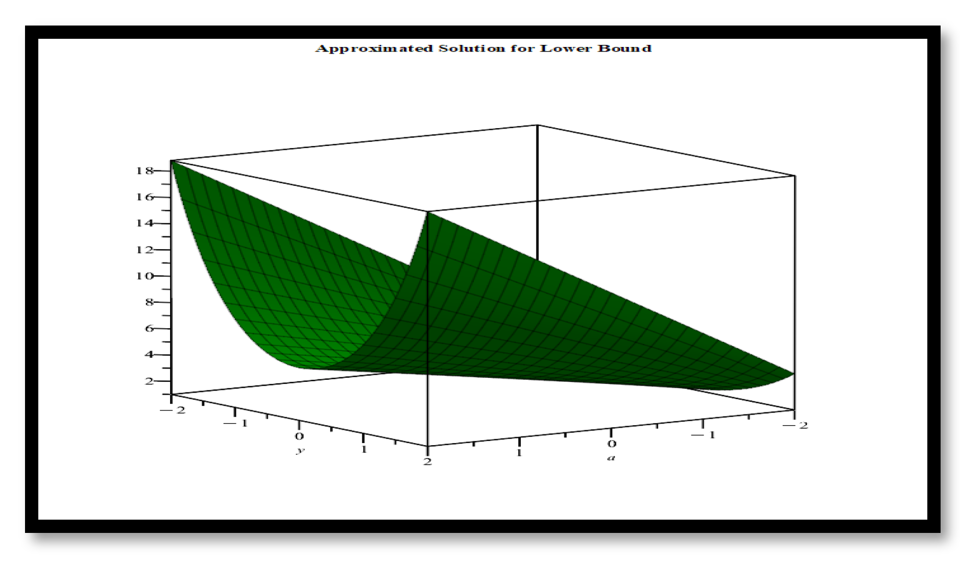
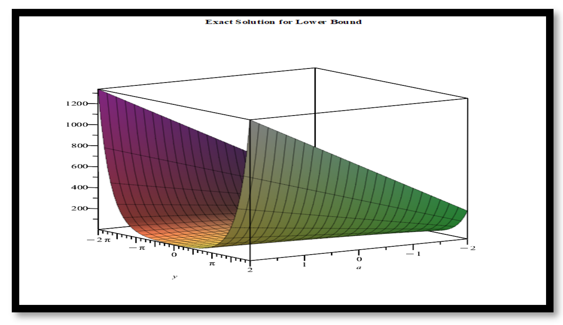
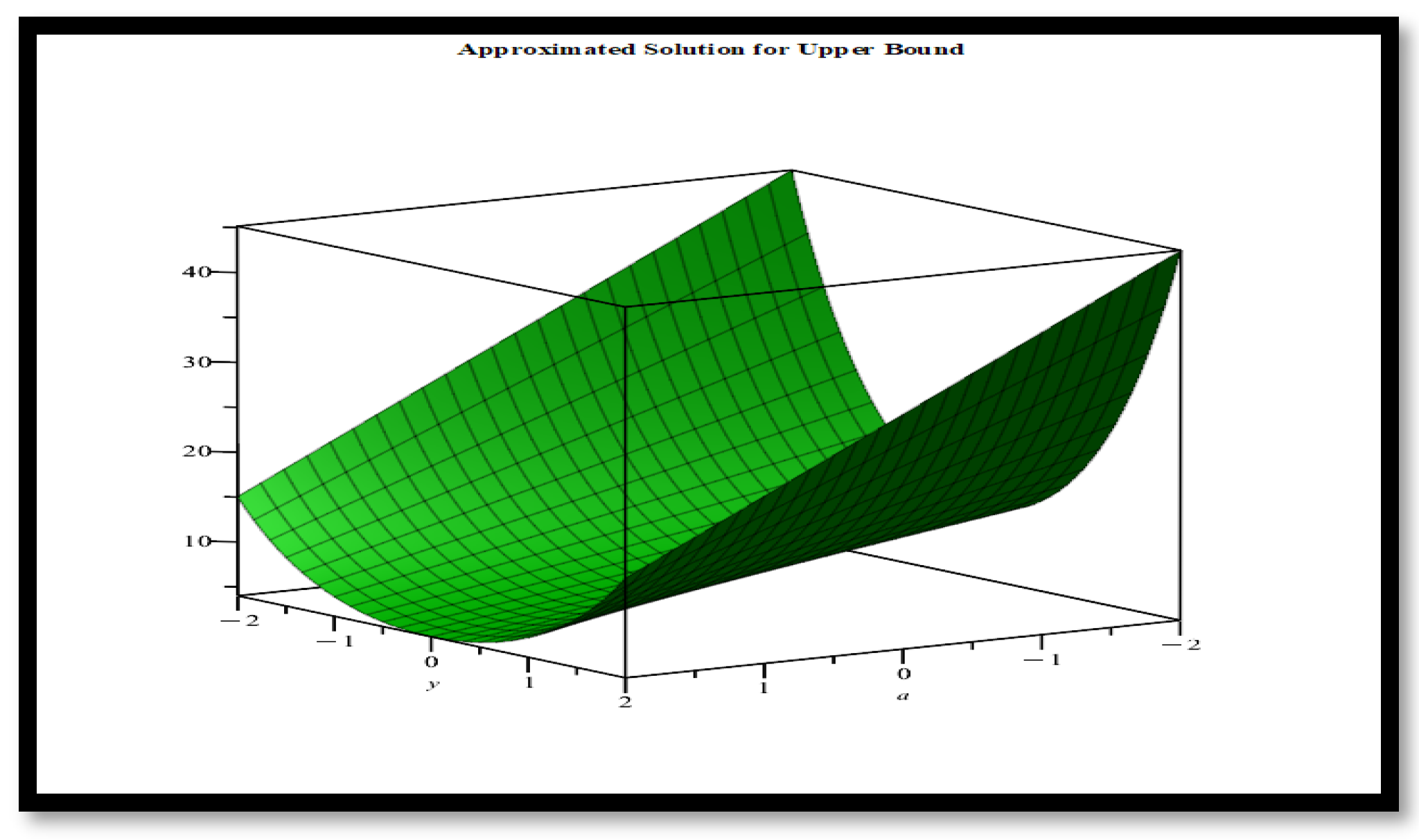
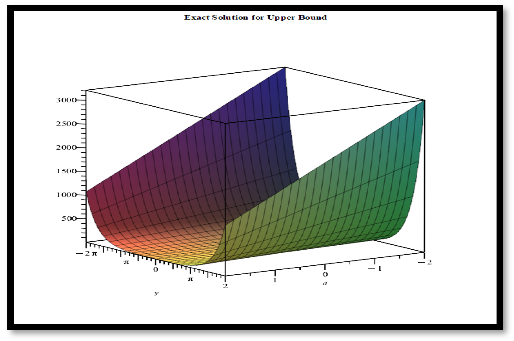
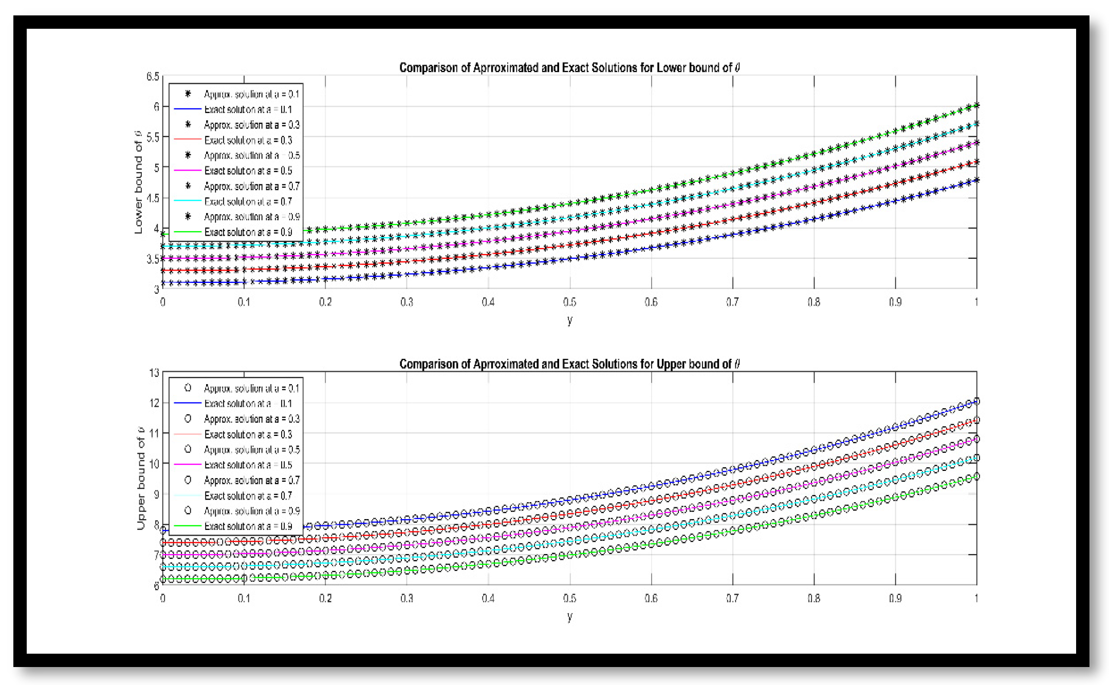
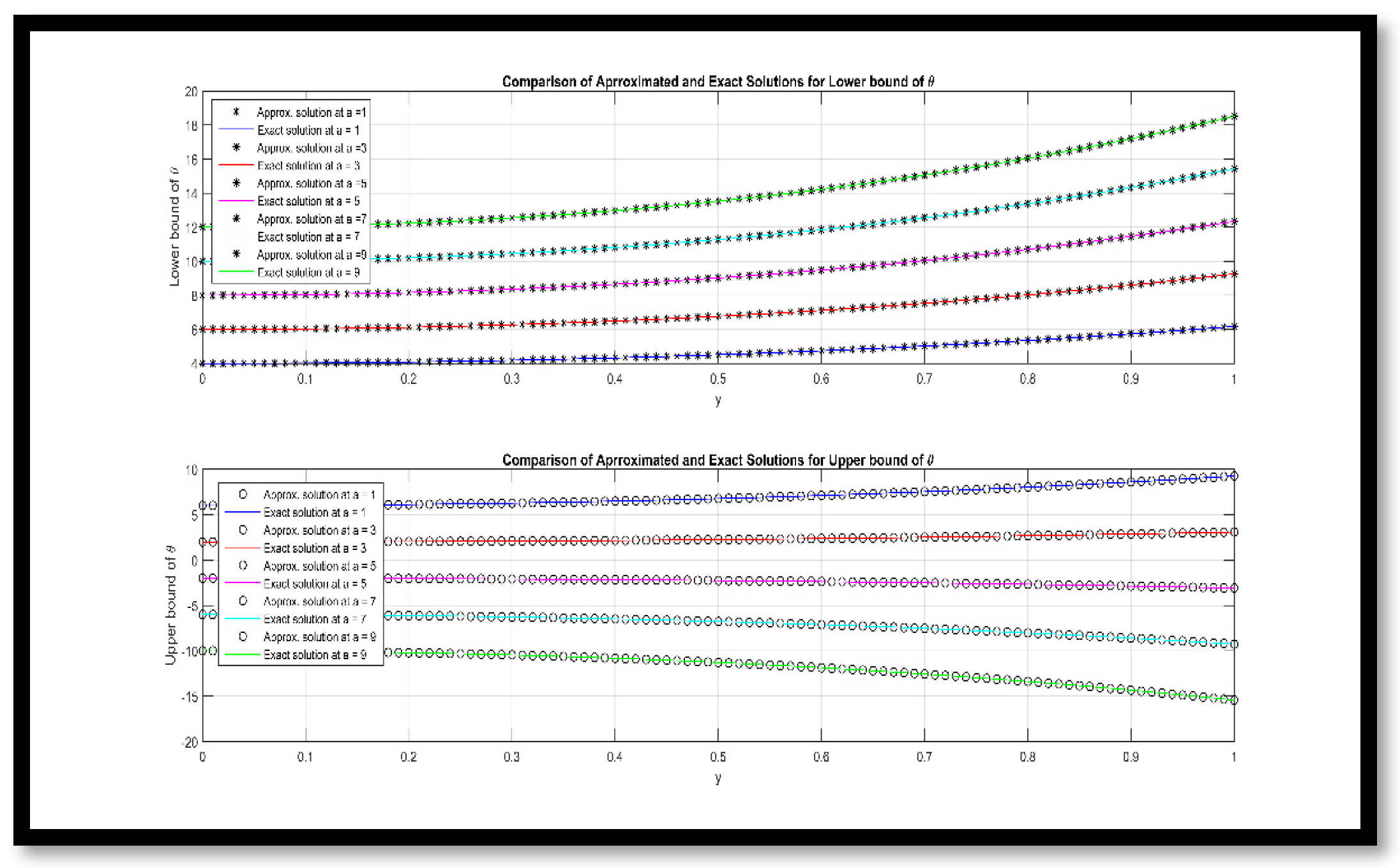
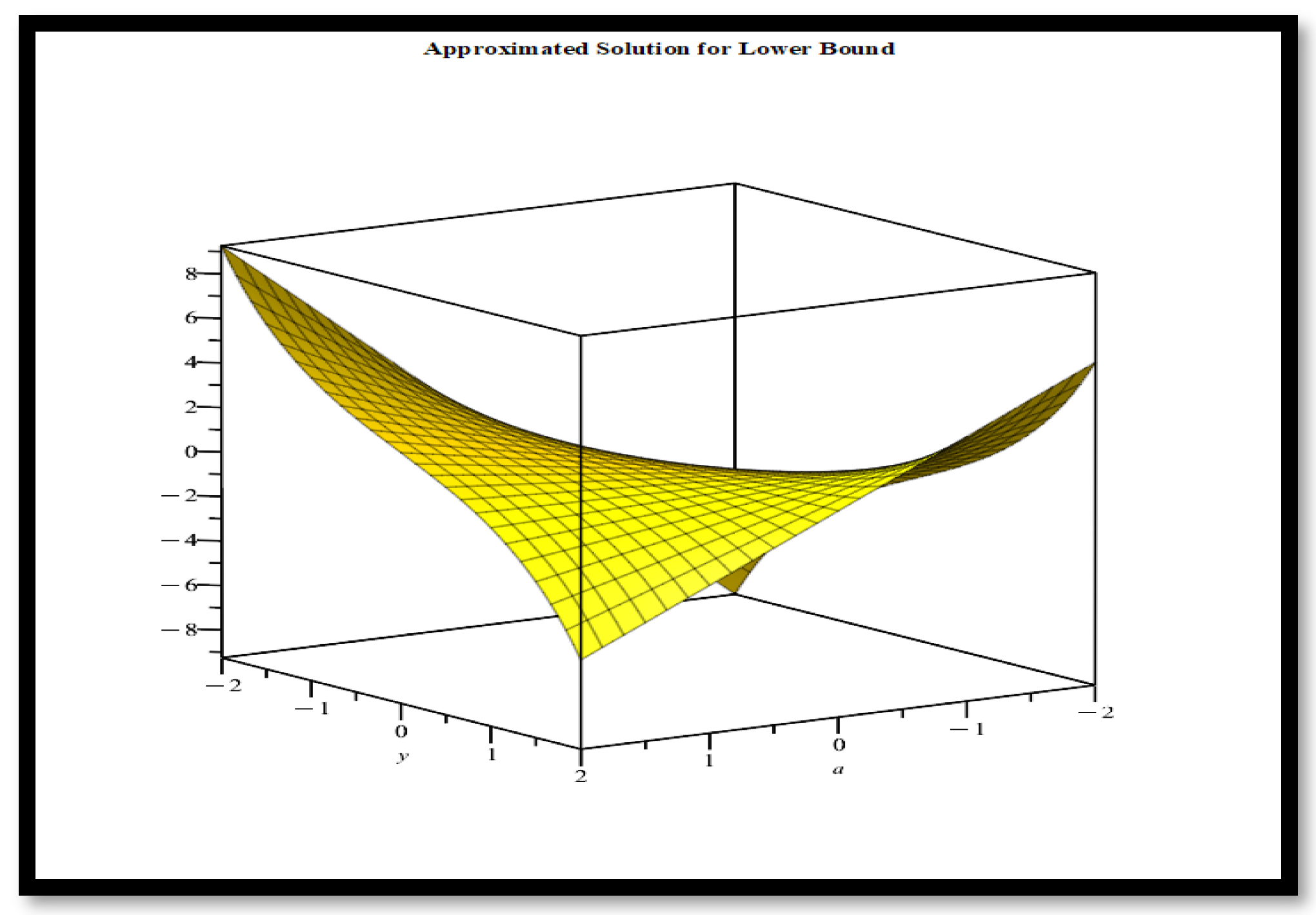
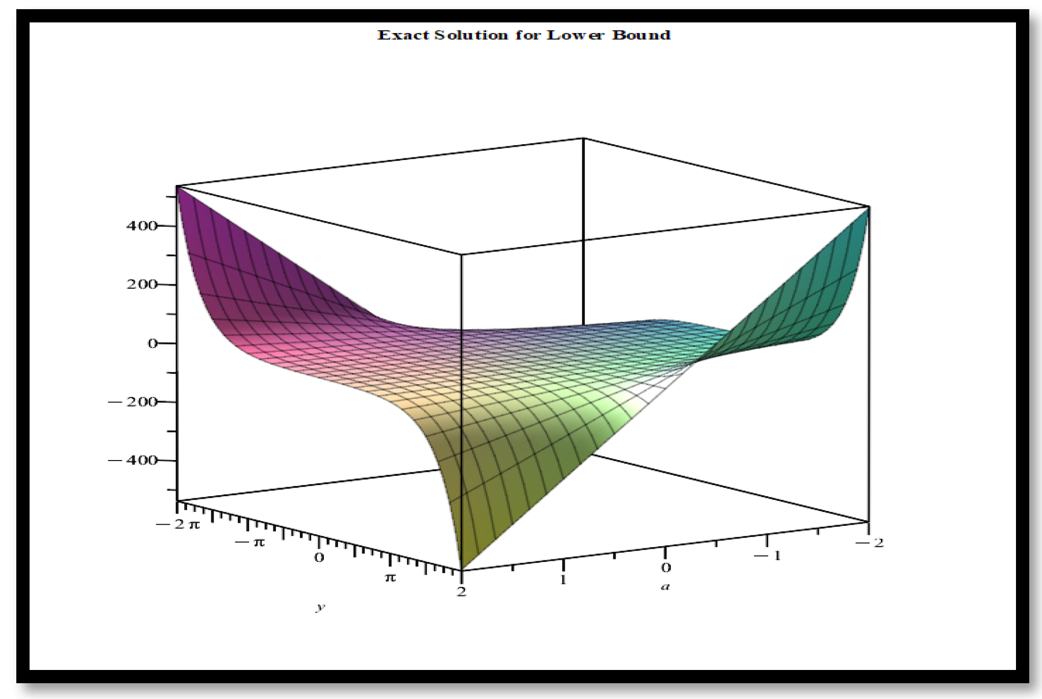
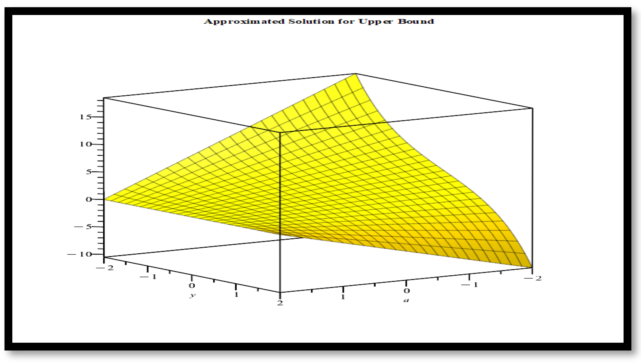
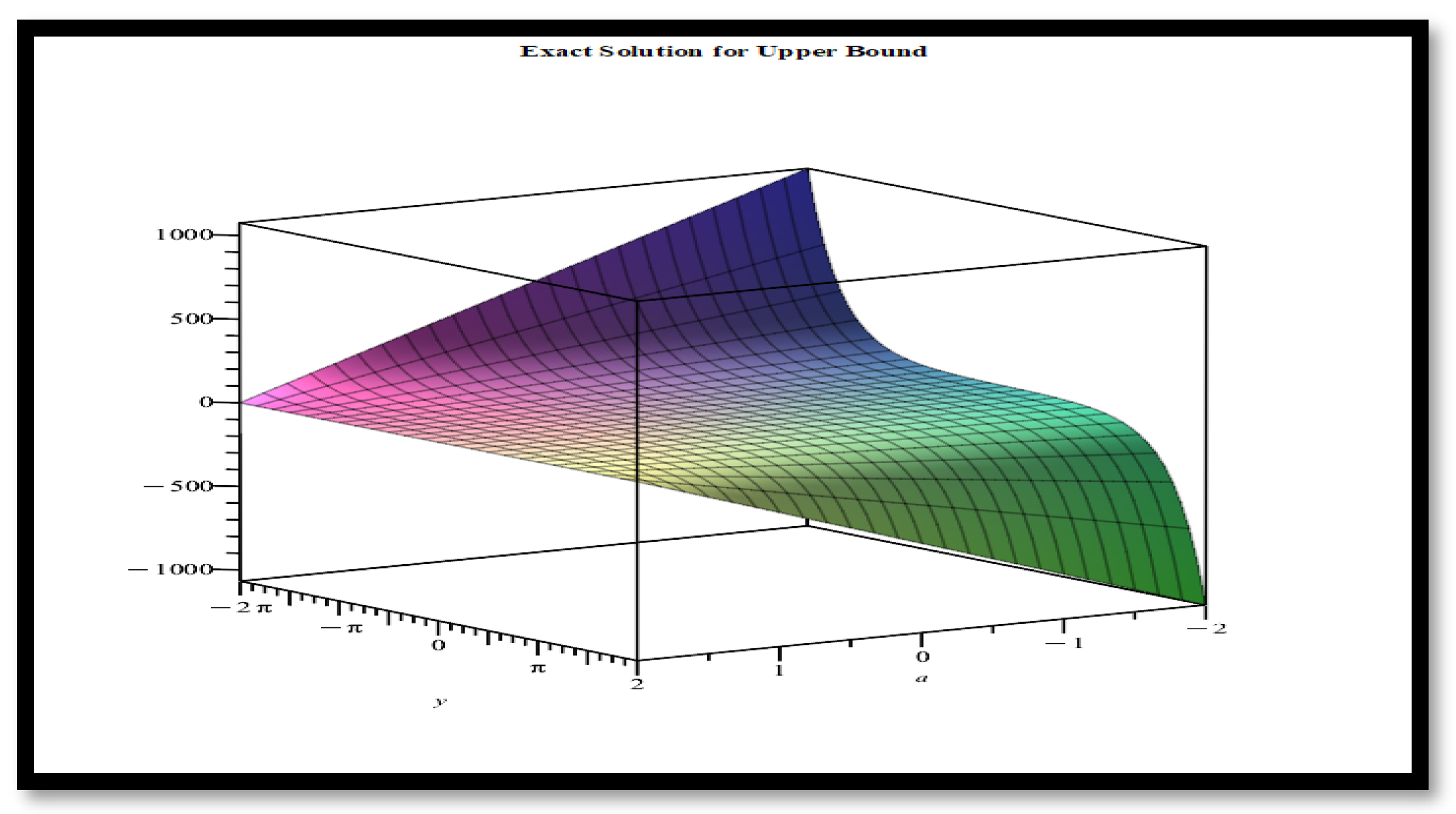
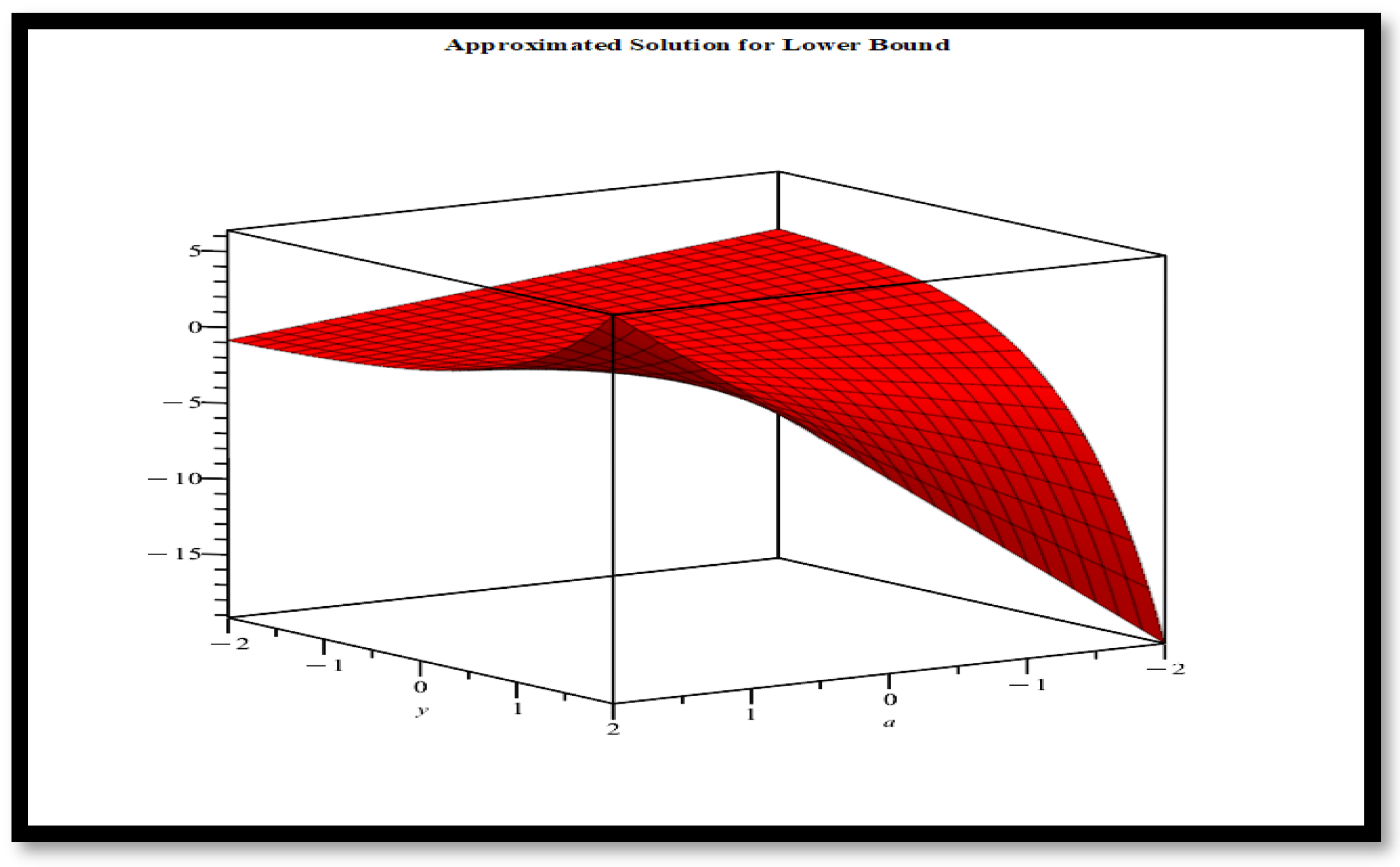
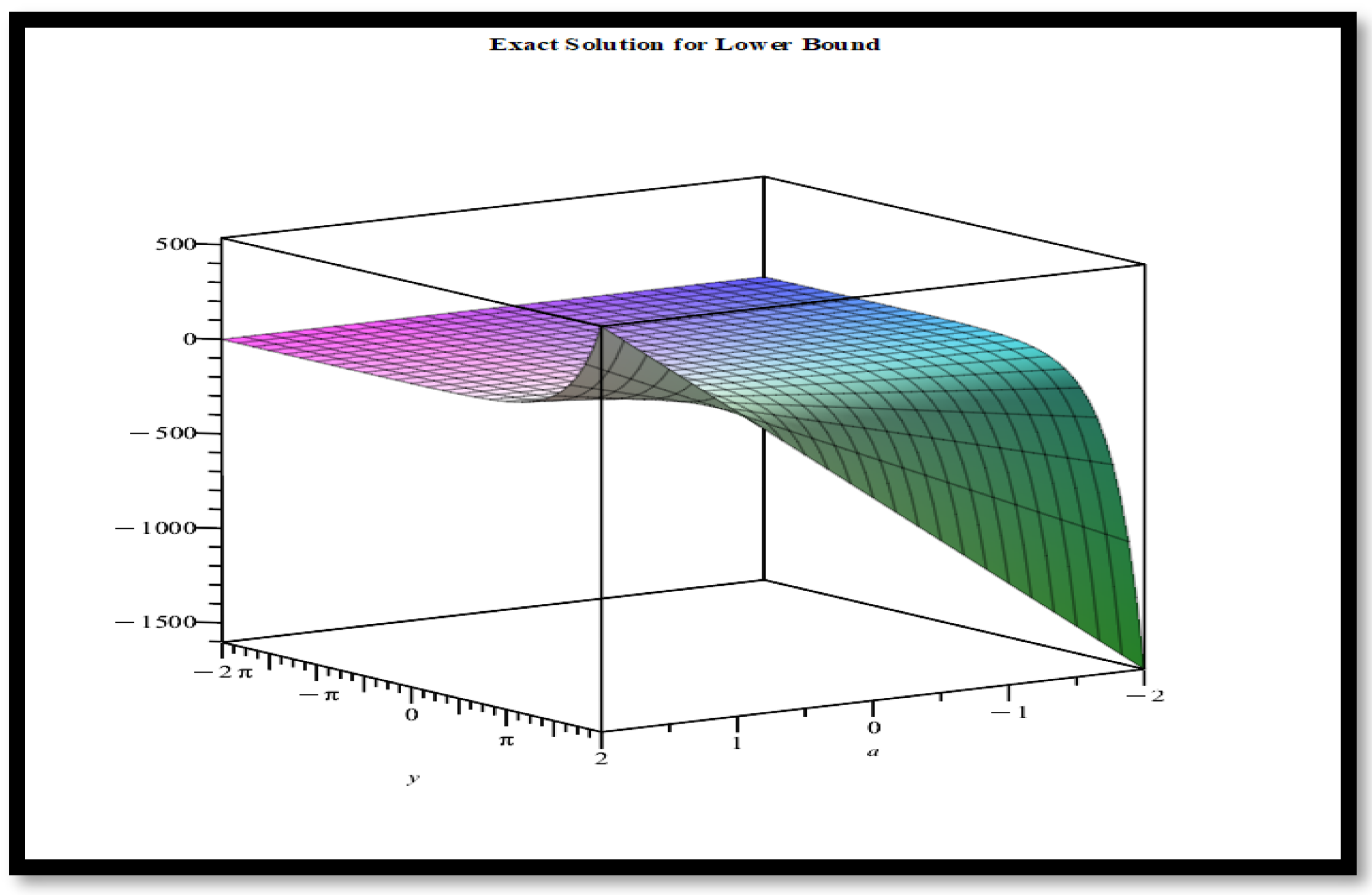
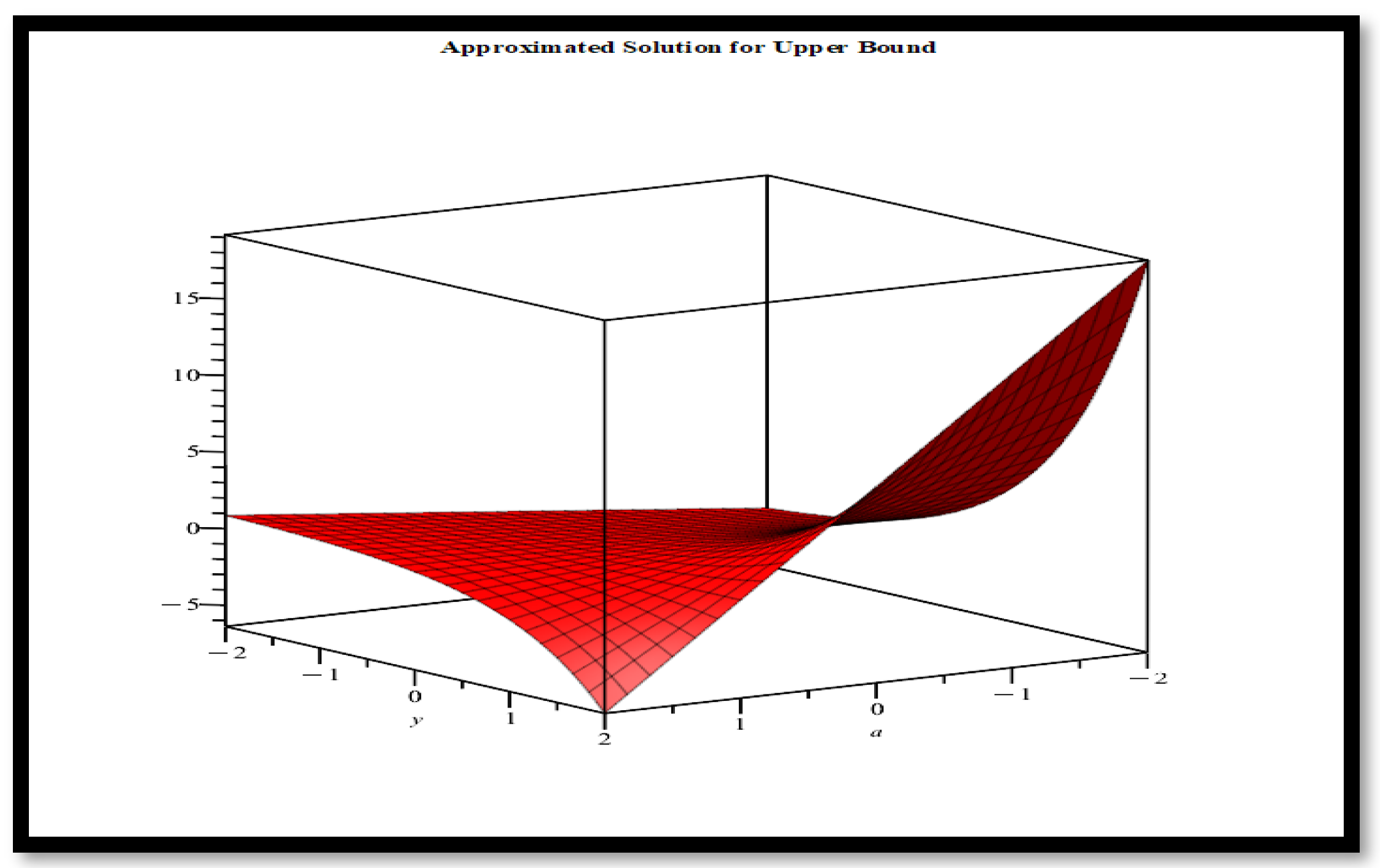
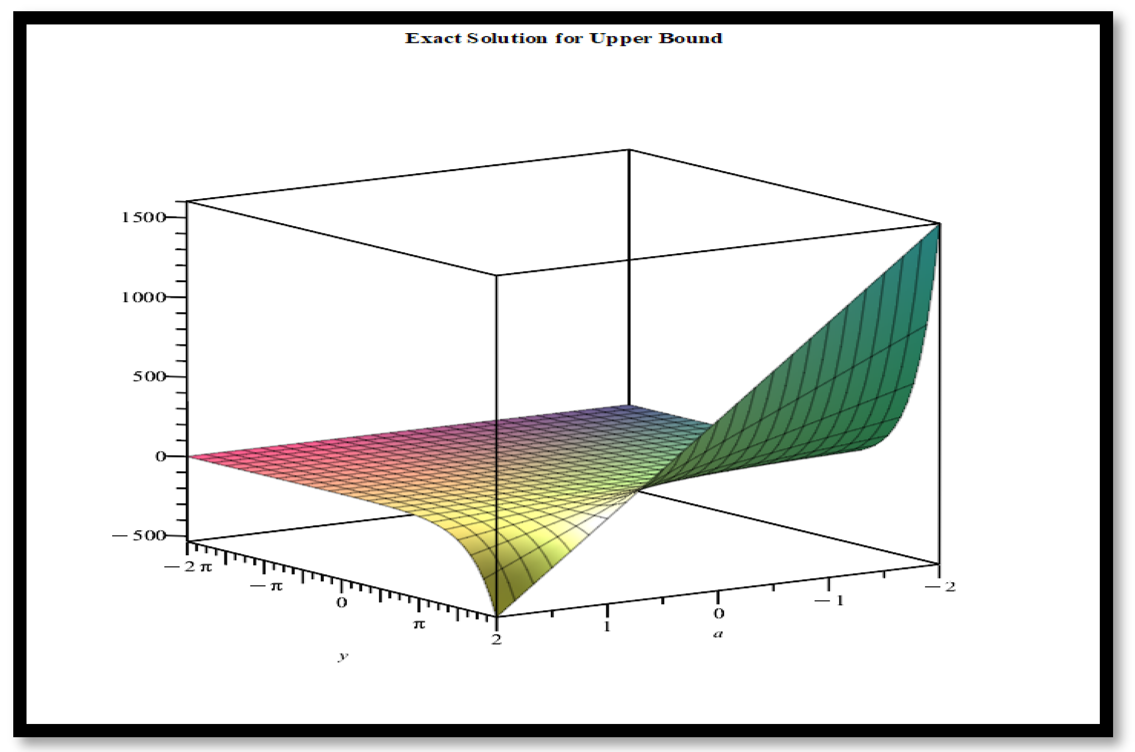
The fuzzy Volterra integral equations were successfully handled in this article using series-type analytical solutions. The Elzaki ADM general approach is utilized for the necessary reasons, and two sequences of upper and lower limit solutions are fetched. Then, we put our proposed technique to the test using three separate cases. It is also emphasized that a simpler method may be used to obtain the same result. The findings show that the Elzaki ADM is an effective tool for solving linear and nonlinear fuzzy integral equation problems. Using this approach, future studies will examine the solutions of the fuzzy Volterra integral equations with various types of crisp and fuzzy kernels. The current regime confirms that semi-analytical regimes are extremely convenient for treating fuzzy differential equations because no discretization error is introduced throughout the process.

It is concluded that the basic idea can easily be extended to similar problems in physical science and engineering. However, numerous fuzzy differential equations may be effectively solved semi-analytically by employing the offered approach. There are still quite a few higher-order fuzzy differential equations that are challenging to handle in the recommended regime, notably the higher-order fuzzy KdV equation and many others. For some discontinuous fuzzy differential equations, the Elzaki ADM cannot be utilized. The Elzaki ADM can only be used for fuzzy differential equations with the initial and boundary conditions since it is an iterative method.

References

1. Alam Khan, N.; Razzaq, O.A.; Ayyaz, M. On the solution of fuzzy differential equations by Fuzzy Sumudu Transform. Nonlinear Eng. 2015, 4, 49–60. [Google Scholar] [CrossRef]
2. Maitama, S.; Zhao, W. Homotopy analysis Shehu transform method for solving fuzzy differential equations of fractional and integer order derivatives. Comput. Appl. Math. 2021, 40, 86. [Google Scholar] [CrossRef]
3. Khastan, A.; Bahrami, F.; Ivaz, K. New results on multiple solutions for th-order fuzzy differential equations under generalized differentiability. Bound. Value Probl. 2009, 2009, 1–13. [Google Scholar] [CrossRef]
4. Salahshour, S.; Allahviranloo, T. Applications of fuzzy Laplace transforms. Soft Comput. 2013, 17, 145–158. [Google Scholar] [CrossRef]
5. Allahviranloo, T.; Abbasbandy, S.; Salahshour, S.; Hakimzadeh, A. A new method for solving fuzzy linear differential equations. Computing 2011, 92, 181–197. [Google Scholar] [CrossRef]
6. Salgado, S.A.B.; Esmi, E.; Sánchez, D.E.; de Barros, L.C. Solving interactive fuzzy initial value problem via fuzzy Laplace transform. Comput. Appl. Math. 2021, 40, 26. [Google Scholar] [CrossRef]
7. Ullah, A.; Ullah, Z.; Abdeljawad, T.; Hammouch, Z.; Shah, K. A hybrid method for solving fuzzy Volterra integral equations of separable type kernels. J. King Saud Univ.-Sci. 2021, 33, 101246. [Google Scholar] [CrossRef]
8. Alidema, A.F. Applications of Double Fuzzy Sumudu Adomain Decompositon Method for Two-dimensional Volterra Fuzzy Integral Equations. Eur. J. Pure Appl. Math. 2022, 15, 1363–1375. [Google Scholar] [CrossRef]
9. Prakash, A.; Veeresha, P.; Prakasha, D.G.; Goyal, M. A homotopy technique for a fractional order multi-dimensional telegraph equation via the Laplace transform. Eur. Phys. J. Plus 2019, 134, 19. [Google Scholar] [CrossRef]
10. Shah, N.A.; Alyousef, H.A.; El-Tantawy, S.A.; Shah, R.; Chung, J.D. Analytical Investigation of Fractional-Order Korteweg–De-Vries-Type Equations under Atangana–Baleanu–Caputo Operator: Modeling Nonlinear Waves in a Plasma and Fluid. Symmetry 2022, 14, 739. [Google Scholar] [CrossRef]
11. Gao, W.; Veeresha, P.; Prakasha, D.G.; Baskonus, H.M.; Yel, G. A powerful approach for fractional Drinfeld–Sokolov–Wilson equation with Mittag-Leffler law. Alex. Eng. J. 2019, 58, 1301–1311. [Google Scholar] [CrossRef]
12. Prakasha, D.G.; Veeresha, P.; Rawashdeh, M.S. Numerical solution for (2 + 1)-dimensional time-fractional coupled Burger equations using fractional natural decomposition method. Math. Methods Appl. Sci. 2019, 42, 3409–3427. [Google Scholar] [CrossRef]
13. Shah, N.A.; Agarwal, P.; Chung, J.D.; El-Zahar, E.R.; Hamed, Y.S. Analysis of Optical Solitons for Nonlinear Schrödinger Equation with Detuning Term by Iterative Transform Method. Symmetry 2020, 12, 1850. [Google Scholar] [CrossRef]
14. Ali, Z.; Rabiei, F.; Hosseini, K. A fractal–fractional-order modified Predator–Prey mathematical model with immigrations. Math. Comput. Simul. 2023, 207, 466–481. [Google Scholar] [CrossRef]
15. Ou, W.; Xu, C.; Cui, Q.; Liu, Z.; Pang, Y.; Farman, M.; Ahmad, S.; Zeb, A. Mathematical study on bifurcation dynamics and control mechanism of tri-neuron bidirectional associative memory neural networks including delay. Math. Methods Appl. Sci. 2023. [Google Scholar] [CrossRef]
16. Li, P.; Gao, R.; Xu, C.; Li, Y.; Akgül, A.; Baleanu, D. Dynamics exploration for a fractional-order delayed zooplankton–phytoplankton system. Chaos Solitons Fractals 2023, 166, 112975. [Google Scholar] [CrossRef]
Figure 1. Approximated solution of the lower bound regarding Example 1.
Fractalfract 07 00650 g001
Figure 2. Exact solution of the lower bound regarding Example 1.
Fractalfract 07 00650 g002
Figure 3. Approximated solution of the upper bound regarding Example 1.
Fractalfract 07 00650 g003
Figure 4. Exact solution of the upper bound regarding Example 1.
Fractalfract 07 00650 g004
Figure 5. Comparison of the approx. and exact solutions for lower and upper bounds at a = 0.1, 0.3, 0.5, 0.7, and 0.9 regarding Example 1.
Fractalfract 07 00650 g005
Figure 6. Comparison of the approx. and exact solutions for lower and upper bounds at a = 1, 3, 5, 7, and 9 regarding Example 1.
Fractalfract 07 00650 g006
Figure 7. Approximated solution for lower bound regarding Example 2.
Fractalfract 07 00650 g007
Figure 8. Exact solution for lower bound regarding Example 2.
Fractalfract 07 00650 g008
Figure 9. Approximated solution for upper bound regarding Example 2.
Fractalfract 07 00650 g009
Figure 10. Exact solution for upper bound regarding Example 2.
Fractalfract 07 00650 g010
Figure 11. Approximated solution for lower bound regarding Example 3.
Fractalfract 07 00650 g011
Figure 12. Exact solution for lower bound regarding Example 3.
Fractalfract 07 00650 g012
Figure 13. Approximated solution for upper bound regarding Example 3.
Fractalfract 07 00650 g013
Figure 14. Exact solution for upper bound regarding Example 3.
Fractalfract 07 00650 g014