An Adaptive Selection Method for Shape Parameters in MQ-RBF Interpolation for Two-Dimensional Scattered Data and Its Application to Integral Equation Solving

Abstract

The paper proposes an adaptive selection method for the shape parameter in the multi-quadratic radial basis function (MQ-RBF) interpolation of two-dimensional (2D) scattered data and achieves good performance in solving integral equations (O-MQRBF). The effectiveness of MQ-RBF interpolation for 2D scattered data largely depends on the choice of the shape parameter. However, currently, the most appropriate parameter is chosen by empirical techniques or trial and error, and there is no widely accepted method. Fourier transform can linearly represent 2D scattering data as a combination of sine and cosine functions. Therefore, the paper employs an improved stochastic walk optimization algorithm to determine the optimal shape parameters for sine functions and their linear combinations, generating a dataset. Based on this dataset, the paper trains a particle swarm optimization backpropagation neural network (PSO-BP) to construct an optimal shape parameter selection model. The adaptive model accurately predicts the ideal shape parameters of the Fourier expansion of 2D scattering data, significantly reducing computational cost and improving interpolation accuracy. The adaptive method forms the basis of the O-MQRBF algorithm for solving one-dimensional integral equations. Compared with traditional methods, this algorithm significantly improves the precision of the solution. Overall, this study greatly facilitates the development of MQ-RBF interpolation technology and its widespread use in solving integral equations.

1. Introduction

The prevalence of scattered data problems is increasing in industries such as engineering design and financial analysis due to the consistent evolution of science and technology. One well-known mesh-free method that is typically utilized to handle this data is radial basis function interpolation. Frank [1] conducted numerous scattered data experiments comparing the accuracy of 29 interpolation methods and concluded that the MQ-RBF interpolation method is the most accurate. It has been pointed out in numerous studies that the accuracy of interpolation is heavily influenced by the shape parameter of the MQ-RBF [2,3].

The MQ-RBF interpolation method was initially proposed by Hardy [4] with the selection of a shape parameter, $c=0.815d$. Here, $d=\frac{1}{N}{\sum }_{i=1}^N{d}_i$ where $d_i$ represents the distance between the ith data point and its closest neighbor. This method provides an adequate fitting effect on terrain problems, leading to numerous researchers exploring the selection of shape parameters in MQ-RBF interpolation. The leave-one-out cross-validation (LOOCV) method, introduced by Rippa [5], has proven to be most influential and effective among these methods. Rippa proposed a cost function to represent the root mean square error (RMSE) between the interpolation function and the original function. The mnbrak and $brent$ in [6] were then used to determine more suitable shape parameters that minimize the cost function. The effectiveness of the method was verified from multiple perspectives, including the condition number of the interpolation matrix and the number and distribution of data points. The method is known to select shape parameters with high accuracy, making it widely used. Since then, many similar MQ-RBF interpolation shape parameter selection methods have appeared. Trahan and Wyatt [7] employed MQ-RBF interpolation in the quantum trajectory method, utilizing leave-one-out cross-validation $\left(LOOCV\right)$ to decide the shape parameter. Wei [8] proposed minimizing the cross-validation root mean squared error $(Cross-RMSE)$ between the interpolation function and the original function to obtain the shape parameter. Their algorithm establishes the initial value $c_{int}=mean\left(d_j\right)$ (where $d_j$ is the minimum distance between sample points) and step size ($l=m/n$, where m is the dimensionality of $x_j$ and n is the number of sample points) beforehand. From there, by searching for the downward trend of error, the direction of error reduction is treated as the direction for parameter iteration until the error ceases to decrease, and the current c value is then regarded as the optimal c. Amirfakhrian [9] introduced an unstructured technique for finding numerical solutions to heat source time-related problems. They combined radial basis functions with the fundamental solution of the heat equation and used them to solve inverse problems at spatial interval boundaries. MQ-RBF compelled them to utilize a generalized cross-validation criterion to locate the shape parameter. There are also some methods [10,11,12,13,14,15,16] that have been developed that significantly advance the selection method research for shape parameters for MQ-RBF interpolation. However, many individuals still encounter challenges. Specifically, selecting the initial shape parameter does not guarantee the best parameters when addressing scattered data problems. This often necessitates time-consuming trial and error or empirical methods to determine the most effective parameters. Unfortunately, these methods can be inefficient and negatively impact the accuracy of interpolation, which can limit the applicability of determined shape parameters. As such, developing a self-adaptive selection method for the shape parameter of MQ-RBF interpolation holds both significant theoretical and practical importance.

This study is intended to develop an optimal shape-parameter-selection model for MQ-RBF interpolation, initially applied to sine functions and their linear combinations. Subsequently, the model is adapted for the Fourier expansion of two-dimensional scattered data, and its efficacy is validated through numerical experiments. It promotes the wide application of the MQ-RBF interpolation method.

Many scientific and engineering problems can be modeled mathematically through integral equations. Compared to differential equations, integral equations are capable of representing both initial and boundary values in the same equation. Moreover, the relative error incurred in numerical integral calculations is much lower compared to the numerical values. Currently, various numerical approaches are being developed to solve integral equations. One such approach [17] is the Galerkin method, or collocation method, which utilizes the Haar wavelet function to solve the first kind of linear Fredholm equation. Meanwhile, the Haar wavelet [18] is used to solve one-dimensional nonlinear equations. Likewise, the Daubechie wavelet and Galerkin method [19] are used to solve the second kind of linear Volterra equation. On the other hand, Maleknejad put forward many methods for different types of one-dimensional integral equations, and the Sinc function collocation method [20,21] is applied for solving one-dimensional linear and nonlinear Fredholm equations of the first kind. The improved block pulse function method [22] is utilized to solve the Volterra integral equation of the first kind and the nonlinear Fredholm equation. The combination of the block pulse function and Taylor series [23] is used to solve the Fredholm-Volterra equation. Polynomial approximation [24] can solve the second kind of Fredholm integral equation of smooth kernel function. These methods mostly use the series form, the Chebyshev polynomial, or the wavelet function, but they have the problem of unstable interpolation or poor accuracy. On the other hand, MQ-RBF shows high interpolation accuracy and good stability in solving one-dimensional integral equations [25]. However, appropriate shape parameters are needed for MQ-RBF to ensure accurate solutions. Choosing the shape parameters based solely on experience and trial and error can be inconvenient. Therefore, this paper proposes an adaptive selection method to identify suitable shape parameters for MQ-RBF and applies it successfully to one-dimensional integral equations. The performance of this method is evaluated through numerical simulation of various one-dimensional integral equations.

2. Algorithm for Selecting Shape Parameters in MQ-RBF Interpolation

2.1. MQ-RBF Interpolation

According to E.M. Stein and G. Weiss [16], a radial basis function ($\phi \left(x\right)$) is a real-valued function whose value is solely determined by the distance from the origin. If $\left|x_1\right|=\left|x_2\right|$, then $\phi \left(x_1\right)$ would be equal to $\phi \left(x_2\right)$.

Table 1. RBF.

Name	$\mathit{\phi }\left(\mathit{r}\right)$
Gaussian	$\phi \left(r\right)=e^{-c^2{r}^2}$
Markov	$\phi \left(r\right)=e^{-c\left|r\right|}$
Multiquadric	$\phi \left(r\right)=\sqrt{c^2+r^2}$
Inverse multiquadric	$\phi \left(r\right)=\frac{1}{\sqrt{c^2+r^2}}$

illustrates the commonly employed radial basis functions.

The function is defined as follows [26]:

$$\tilde{f}\left(x\right)=\sum _{j=1}^N{\lambda }_j{\phi }_j\left(r\right)$$

(1)

Here, ${\lambda }_j$ is the jth weight of the sample point, and N refers to the number of sample points. ${\phi }_j\left(r\right)$ represents the basis function, as given by

$${\phi }_j\left(x\right)=\sqrt{{\left(∥x-x_j∥\right)}^2+c^2}$$

(2)

c is a shape parameter. When employing MQ-RBF interpolation, it determines the efficacy of the interpolation. $x_j$ is the jth sample point. As the basis function $\tilde{f}\left(x\right)$ passes through the sample points, we obtain the equation:

$$\tilde{f}\left(x_j\right)=F\left(x_j\right),j=1,2,\cdots N$$

(3)

The basis function matrix ${\mathrm{\Psi }}_{N\times N}$ can be defined as shown below:

$${\mathrm{\Psi }}_{N\times N}=\left[\begin{array}{ccc}{\phi }_{11}& \cdots & {\phi }_{1N}\\ ⋮& \ddots & ⋮\\ {\phi }_{N1}& \cdots & {\phi }_{NN}\end{array}\right]$$

(4)

where ${\phi }_{ij}$ is the basis function about the sample points and the jth sample point:

$${\phi }_{ij}\left(x\right)=\sqrt{{\left(∥x_i-x_j∥\right)}^2+c^2},i=1,2,\cdots N$$

(5)

Furthermore, let W denote the weight vector ${\lambda }_j$ and F denote the vector of $f\left(x_j\right)$; we end up obtaining

$$F=\left[\mathrm{\Psi }\right]\left[W\right]$$

(6)

2.2. Algorithm Selection

The present study employs optimization algorithms to determine the shape parameters of MQ-RBF interpolation for sine functions. This approach offers several advantages, including cost reductions as well as improved accuracy of interpolation. The optimization problem that represents the selection of shape parameters in MQ-RBF is as follows:

$$E_{max}\left(c\right)=\underset{x\in \left(a,b\right)}{max}|s\left(x,c\right)-f\left(x\right)|$$

(7)

$$\left\{\begin{array}{cc}\hfill & Find{c}_{opt}\hfill \\ \hfill & min{E}_{max}\left(c\right)\hfill \end{array}\right.$$

(8)

The parameters of the interpolation include the interpolation basis function $s\left(x,c\right)$, the interpolation primitive function $f\left(x\right)$, the maximum error $Emax\left(c\right)$, and the required optimal shape parameter $copt$ for the interpolation.

To determine the ideal optimization algorithm for determining MQ-RBF’s interpolation shape parameters in sine functions, we utilized different optimization approaches [27,28,29,30,31], such as Gradient Descent (GD), Newton-Raphson method (NR), Genetic Algorithm (GA), Tabu Search (TS), and Random Walk (RW), for MQ-RBF interpolation of numerous sine functions. The leave-one-out cross-validation method [5] was utilized in our study to select the initial shape parameter of Function (9), which yielded a value of 0.4133. After a series of experiments, we identified the optimal settings for the initial shape parameter optimization using different algorithms. These settings consist of a learning rate of 0.1 for GD, a population size of 10 for GA, a taboo length of 10 for TS, and 10 walks for RW. We compared the performance of these algorithms in terms of interpolation accuracy, computation time, and the number of iterations required to reach the optimal shape parameters, with all algorithms being set to a maximum iteration of 20. The results provided us with important insights regarding the optimization algorithms’ capability to identify the optimal shape parameters.

Table 2. Comparison of algorithm effects.

Algorithm	${\mathit{c}}_{\mathit{opt}}$	MaxError	Run Time (s)	Number of Iterations
GD	0.64027	$5.98\times {10}^{-7}$	0.2855	20
NR	1.07542	$6.52\times {10}^{-7}$	0.2569	20
GA	0.54031	$2.26\times {10}^{-7}$	0.6937	16
TS	0.48296	$4.05\times {10}^{-7}$	0.4016	15
RW	0.54027	$2.28\times {10}^{-7}$	0.2601	16

highlights the results of Function (9).

$$y=sin\left(\pi x\right)$$

(9)

According to our experimental results, GA and TS were found to produce relatively small shape parameter errors and to require fewer iterations to identify the optimal shape parameters compared to other algorithms when initially configured with the same number of iterations and shape parameters. However, these algorithms require more computation time. In contrast, GD and NR exhibit faster training but produce larger shape parameter errors when the maximum iteration is reached. On the other hand, while ensuring high interpolation accuracy, RW requires a relatively short computation time. Therefore, we recommend using the RW to determine the shape parameter of the MQ-RBF interpolation function for the sine function.

The selection of the optimal shape parameter ($c_{opt}$) using the Random Walk (RW) algorithm involves the following steps:

Step 1: Define $i\left(i=1,2\dots ,M\right)$ as the number of walks, $k\left(k=1,2\dots ,N\right)$ as the number of current iterations, the accuracy $\theta$ for step control, and the accuracy $\epsilon$ for error control. Set k equal to 1 and establish the initial parameter $c_0$.

Step 2: The initial step length for the first walk is ${\lambda }_0$. Every iteration generates a random N-dimensional vector

$u_{ik}=\left(u_1,u_2,\cdots ,u_n\right),u_{ik}\in \left(-q,q\right)$, which is then standardized to derive $u_{ik}^{{}^{\prime }}=\frac{u_{ik}}{\sqrt{{\displaystyle \sum _{j=1}^n}{u_j}^2}}$, satisfying $c_1=c_0+{\lambda }_0{u_{1k}}^{\prime },\cdots ,c_i=c_{i-1}+\lambda {u_{ik}}^{{}^{\prime }}\cdots$.

Step 3: Compute the value of $Emax\left(c_i\right)$:

(1) If $Emax\left(c_i\right)<Emax\left(c_{i-1}\right)$, the ith step is completed. Take $c_i$ as the new initial parameter, reset k to 1, and begin the next walk. The walk process is repeated until $Emax\left(c\right)<\epsilon$ or $i=M$, at which point the algorithm ends.

(2) If $Emax\left(c_i\right)>Emax\left(c_{i-1}\right)$, it indicates that no better parameter than the present one has been found. If $k<N$, return to step 2 to regenerate the random vectors $u_{ik+1},\cdots ,$ $u_{iN-1}$ and continue the search. When $k=N$ and no better parameter is found, the optimal parameter $c_{opt}$ is regarded as in the sphere with a center $c_{i-1}$ and a radius $\lambda$. If $\lambda <\theta$, end the algorithm; otherwise, set $\lambda ={\lambda }_0/2$, go back to step 1, and initiate a new round of walking.

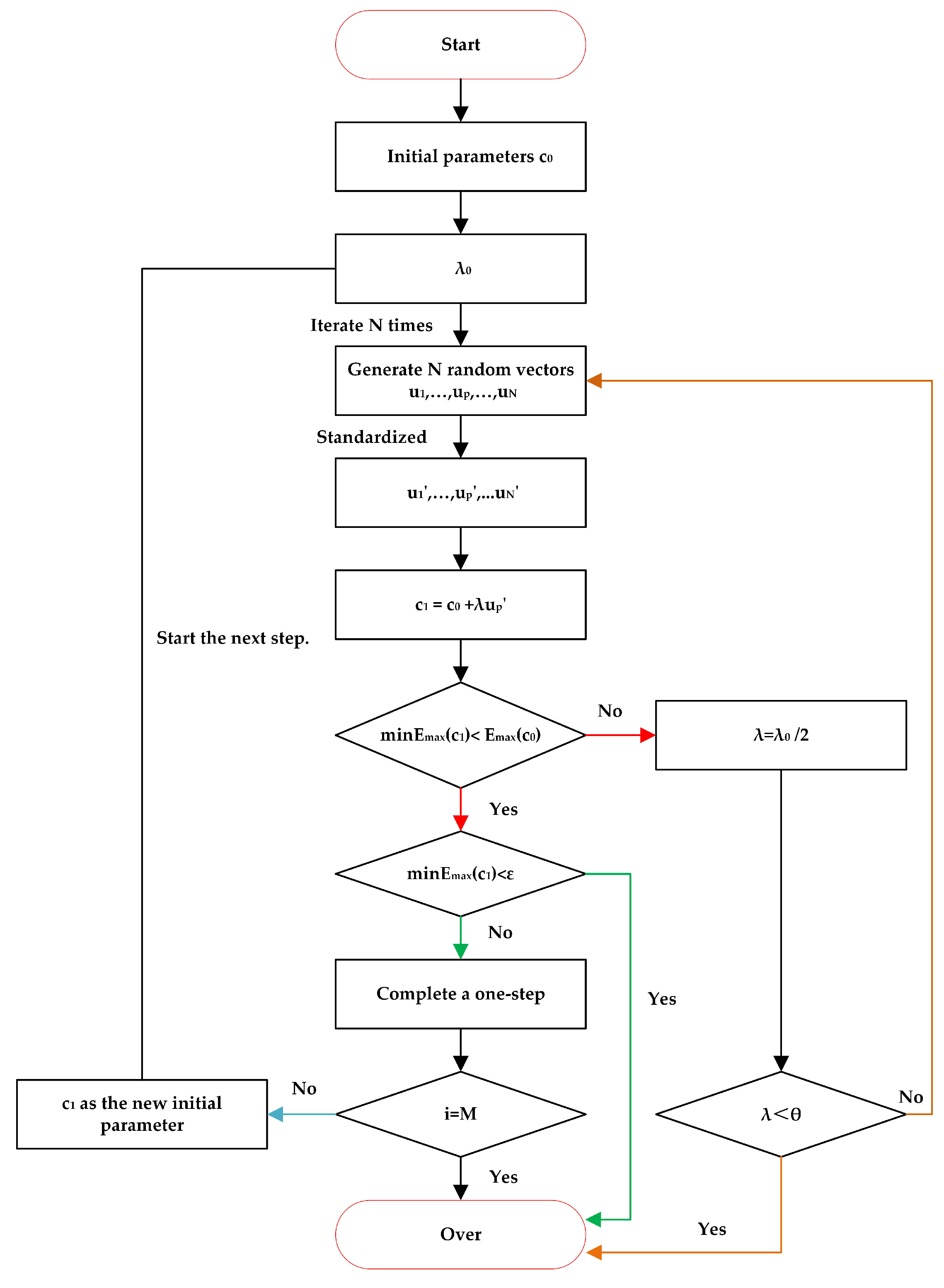
2.3. Improved Random Walk Algorithm

The Random Walk algorithm, however, exhibits some issues in finding parameters. If a superior parameter is discovered in the initial parameter’s neighborhood, the algorithm will advance to the next walk, regardless of whether the iteration meets the specified N times or not. As a result, the outcome may regress into local optimization.

We have made enhancements to the Random Walk algorithm and labeled it the Improved Random Walk Algorithm (IRW). The enhancements are as follows: every walk is iterated for N times, and the parameter registered with the corresponding minimum error in this walk is taken as the starting parameter for the next walk. By incorporating this improvement, the algorithm covers a wider parameter range and offers more directions. Figure 1 displays a flowchart of IRW for determining the best shape parameters.

Table 3. IRW’s result about Equation (9).

Algorithm	${\mathit{c}}_{\mathit{opt}}$	MaxError	Run Time (s)	Number of Iterations
IRW	0.52147	$1.43\times {10}^{-7}$	0.2675	14

presents the interpolation data for the optimal shape parameter selected by the IRW algorithm based on Equation (9) for the purpose of comparison with the results in Table 2. Our validation process has repeatedly shown that the IRW algorithm can identify the optimal shape parameter with minimal iterations, thereby enhancing the interpolation accuracy without significantly increasing the time cost. Furthermore, Figure 2 and Figure 3 demonstrate the impact and absolute error of the MQ-RBF interpolation based on the ideal shape parameters established by the IRW algorithm in Equation (9). These figures indicate that the chosen shape parameters have excellent interpolation effects. The low cost and high precision of the IRW algorithm make it the most suitable choice for our problem as we need to accumulate a large number of data.

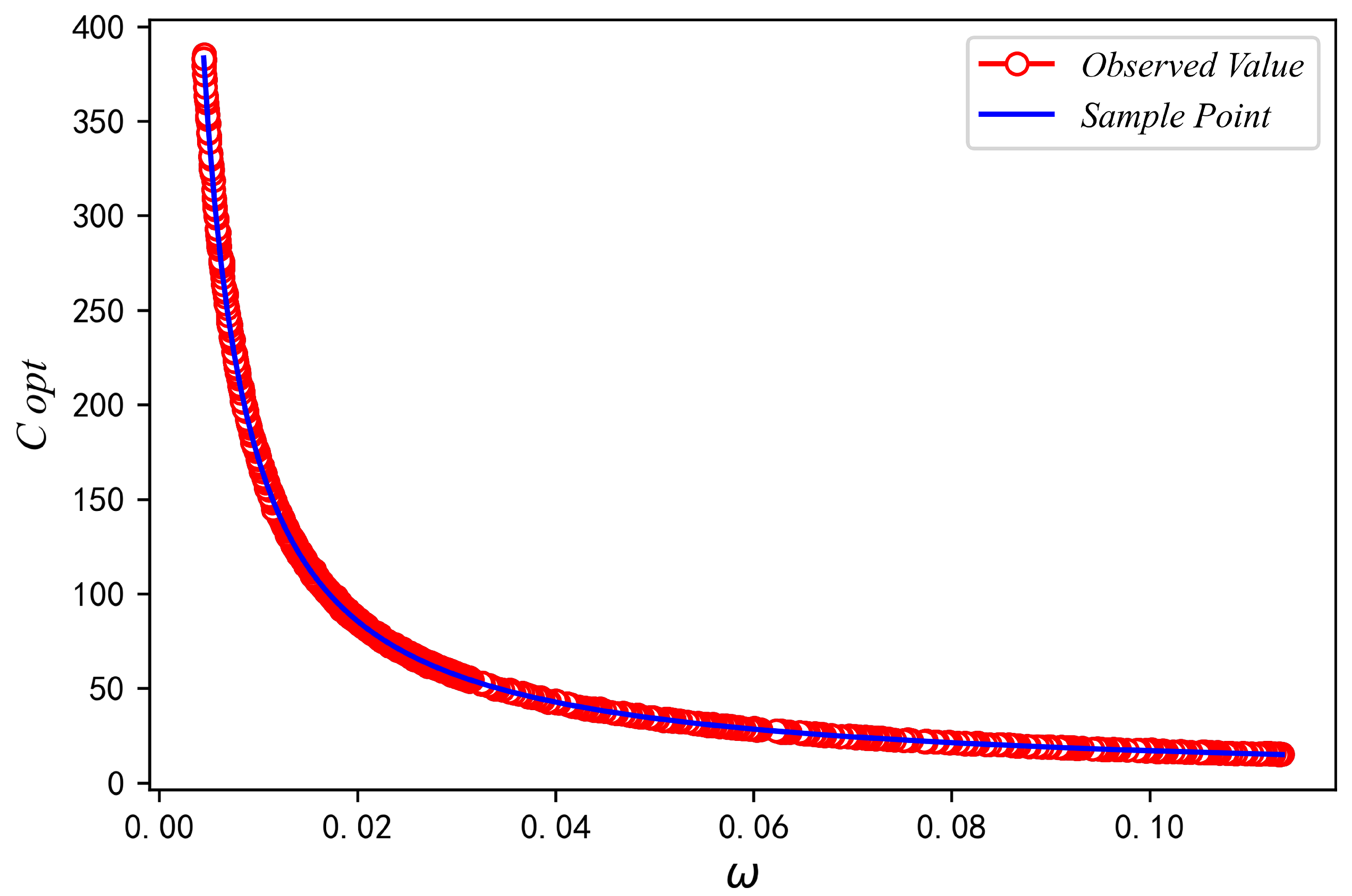
3. Selection Model of the ${\mathit{c}}_{\mathit{opt}}$

3.1. The Relationship between $\omega$ and $c_{opt}$

Sine and cosine functions are collectively referred to as sine functions in practical applications. Their general function expression is as follows:

$$y=Asin(\omega x+\phi )+B$$

(10)

The expression for trigonometric functions includes four parameters, amplitude, offset, initial phase, and angular frequency, denoted as A, B, $\phi$, and $\omega$ respectively. These parameters determine the basic shape of the trigonometric curve. As stated by [7], the basic shape of the MQ-RBF is determined by its parameter c. Our numerous experimental results indicate that A, B, and $\phi$ have negligible influence on the $c_{opt}$, while $\omega$ exerts a profound impact on the $c_{opt}$ [32]. Consequently, the IRW algorithm is employed to explore the relationship between $\omega$ and the $c_{opt}$.

$$f\left(x\right)=sin\left(\omega x\right)$$

(11)

Let $\omega =k\pi (k=2,\cdots ,10)$ in Equation (11); i.e., expand the angular frequency of Equation (9) by a factor of k. Selected experimental results are presented in

Table 4. $\omega =k\pi \left(k=2,\cdots ,10\right)$ experimental results.

$\mathit{\omega }$	${\mathit{c}}_{\mathit{opt}}$	MaxError
$2\pi$	0.26073	$1.43\times {10}^{-7}$
$3\pi$	0.17382	$1.42\times {10}^{-7}$
$4\pi$	0.13036	$1.43\times {10}^{-7}$
$5\pi$	0.10429	$1.45\times {10}^{-7}$
$6\pi$	0.08691	$1.40\times {10}^{-7}$
$7\pi$	0.07449	$1.42\times {10}^{-7}$
$8\pi$	0.06518	$1.41\times {10}^{-7}$
$9\pi$	0.05631	$1.42\times {10}^{-7}$
$10\pi$	0.05142	$1.41\times {10}^{-7}$

.

According to the experimental results, changes in $\omega$ had a minor impact on the interpolation accuracy. When the angular frequency is multiplied by a factor of k, the corresponding $c_{opt}$ decreases by approximately k. Further verification was performed by dividing the $\omega$ by a factor of k$(k=2,\cdots ,10)$, and some of the experimental results are presented in

Table 5. $\omega =\frac{\pi }{k}(k=2,\cdots ,10)$ experimental results.

$\mathit{\omega }$	${\mathit{c}}_{\mathit{opt}}$	MaxError
$\pi /2$	1.04294	$1.43\times {10}^{-7}$
$\pi /3$	1.56441	$1.42\times {10}^{-7}$
$\pi /4$	2.08588	$1.46\times {10}^{-7}$
$\pi /5$	2.60735	$1.42\times {10}^{-7}$
$\pi /6$	3.12882	$1.41\times {10}^{-7}$
$\pi /7$	3.65029	$1.43\times {10}^{-7}$
$\pi /8$	4.17176	$1.40\times {10}^{-7}$
$\pi /9$	4.69343	$1.43\times {10}^{-7}$
$\pi /10$	5.22458	$1.40\times {10}^{-7}$

.

Numerous numerical experiments have demonstrated an approximate inverse proportionality between variables $\omega$ and $c_{opt}$ for trigonometric functions. The IRW algorithm is employed to select parameters for every individual trigonometric function. Subsequently, the MQ-RBF interpolation shape parameter selection formula of a trigonometric function is fitted using the least-square method [33] based on a large number of data points that correspond to a one-to-one relationship with respect to the results. Figure 4 presents the fitting image of some data, and the resulting formula is Equation (12).

$$c_{opt}=1.712916/\omega +0.1668$$

(12)

3.2. The $c_{opt}$ Selection Model for the Linear Combination of Sine Functions

3.2.1. Establishment of the Data Set and Selection of Regression Model

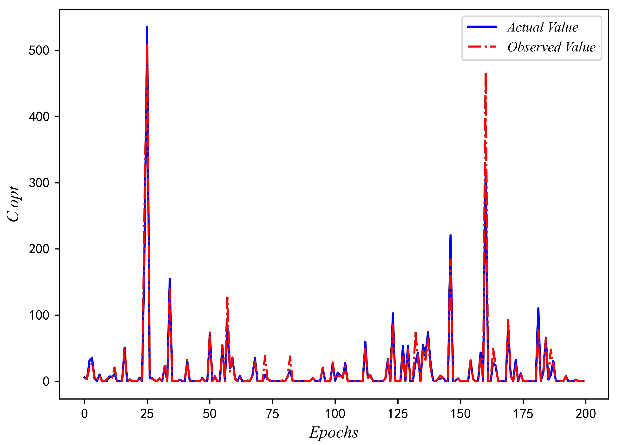
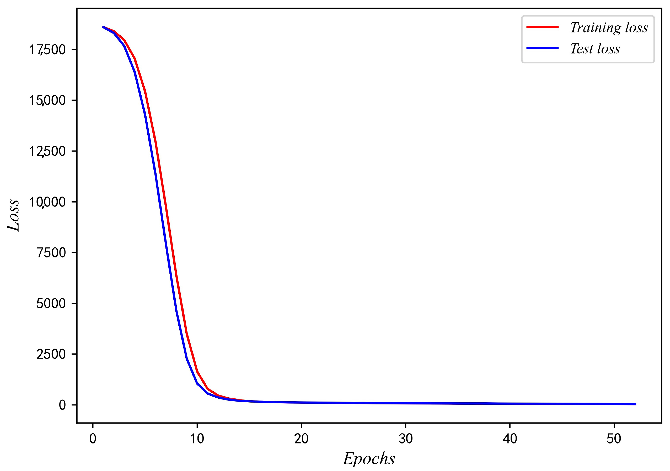
A linear combination of trigonometric functions can be expressed mathematically as follows [34]:

$$y=\sum _{k=1}^N{A}_{k}sin({\omega }_{k}x+{\theta }_k)$$

(13)

The number of terms in the linear combination of trigonometric functions is denoted by N, and the amplitude, angular frequency, and initial phase of the kth term’s trigonometric function are represented by $A_k$, ${\omega }_k$, and ${\theta }_k$, respectively. The $c_{opt}$ in the MQ-RBF interpolation for linear combinations of trigonometric functions is determined by the IRW algorithm. Experimental research has shown that the angular frequency is the primary determinant of the corresponding $c_{opt}$. Specifically, the highest angular frequency term significantly affects $c_{opt}$ for MQ-RBF interpolation in linear combinations of trigonometric functions. Based on these results, a dataset is proposed that includes the angular frequency of the linear combination of trigonometric functions along with their corresponding $c_{opt}$.

Using the Pandas library in Python 3.10, the angular frequencies and corresponding optimal shape parameters for 1 million linear combinations of sine functions were divided into segments. To generate a training and testing dataset, we conducted three train–test splits with ratios of 7:3, 6:4, and 9:1, respectively. A 6:4 ratio is more suitable for smaller datasets since it can help prevent overfitting. A 7:3 ratio ensures model accuracy while avoiding overfitting and underfitting, making it best suited for moderate-sized datasets. A 9:1 ratio allocates more data for model training, improving model accuracy by allowing for a better understanding of the dataset’s characteristics and patterns. Given the large size of our dataset, we validated and compared the different ratios, ultimately selecting the 9:1 ratio as the most appropriate for our needs.

We trained five models [35,36,37,38,39], namely, Back Propagation Neural Network (BP), Multiple Linear Regression (MLR), Gated Recurrent Unit (GRU) networks, Support Vector Machine (SVM), and Long Short-Term Memory (LSTM), using 900,000 data points as the training set. We compared and evaluated the models using 100,000 data points as the test set. We used three evaluation indices, namely training time, mean square error (MSE), and prediction accuracy. Refer to

Table 6. Comparison of model effects.

Model	Time (Min)	MSE	Accuracy
BP	2014	0.248787	91.7344%
LSTM	2083	1.847632	84.9843%
GRU	1971	2.847412	81.5832%
SVR	2646	7.626251	74.2447%
MLR	1722	18.72263	67.9843%

for results.

Our experimental results show that, despite its shorter training time, MLR exhibits the poorest predictive accuracy, suggesting that there is no clear linear relationship between the data. The performance of SVR in handling large-scale samples results in average training and predictive accuracy. Compared to SVR and LSTM, the BP predicts the shape parameters of linear combinations of trigonometric functions with the highest accuracy, with the same amount of training time. After a comprehensive comparison, we selected the BP to perform shape parameter prediction.

3.2.2. Construction of the $c_{opt}$ Selection Model Based on PSO-BP

The BP is composed of three layers: the input layer, the hidden layer, and the output layer. The signal transmission in the BP progresses forward sequentially through the input layer, hidden layer, and output layer, while its error is propagated backward, starting from the output layer, then the hidden layer, and finally the input layer. The learning ability of the neural network is directly impacted by the number of nodes in the hidden layer, and the formula used to calculate it is as follows:

$$h=\sqrt{l+j}+e$$

(14)

where h represents the number of nodes in the hidden layer, l represents the number of nodes in the input layer, and e is a constant in the range of [1,10] and takes an integer value. The architecture of our BP neural network includes two hidden layers, with 80 and 30 neurons in the first and second hidden layers, respectively. We selected Rectified Linear Unit (ReLU) as our activation function while setting the learning rate to 0.05 and the momentum to 0.9.

Particle Swarm Optimization (PSO) [40] is an optimization algorithm that imitates the predation behavior of birds. Unlike the random gradient descent method used in BP training, PSO is a global optimization algorithm that can find the optimal solution to a problem in the entire region. The algorithm generates a set of random solutions and then updates the particle velocity and position in each iteration to find the optimal solution. The rules for updating the particle velocity and position are as follows:

$$V_i^{k+1}=w{V}_i^{k+1}+c_1{r}_1(p_{best}-X_i^k)+c_2{r}_2(g_{best}-X_i^k)$$

(15)

$$X_i^{k+1}=X_i^k+V_i^{k+1}$$

(16)

The variables $V_i^k$ and $X_i^k$ denote the velocity and position of particle i during the kth iteration. The variable $\omega$ corresponds to the inertia factor. The variable $c_1$ corresponds to the individual learning factor. The variable $c_2$ corresponds to the social learning factor. The variables $r_1$ and $r_2$ correspond to random numbers in the range [0,1]. The variables $p_{best}$ and $g_{best}$ indicate the best positions found so far by the current single particle and by all particles, respectively.

The BP can perform the nonlinear mapping from input to output, but it is prone to reaching a local minimum after a specific number of iterations. PSO can fully utilize the nonlinear application of BP and overcome the issue of the slow convergence of weights in the BP training neural network, which can easily cause it to fall into local optima.

Table 7. Effect evaluation of PSO-BP.

Model	Evaluation Index	Result
	Time (min)	2083
PSO-BP	MSE	0.1925473
	Accuracy	97.2154%

presents the evaluation results of the Particle Swarm Optimization Backpropagation model (PSO-BP). Without imposing significant time costs, the model demonstrates significant improvements in MSE and prediction accuracy.

In our study, we propose using Particle Swarm Optimization (PSO) as the optimizer to enhance the effectiveness of our model. The PSO algorithm is configured with the following parameters: swarm size, maximum number of iterations, inertia weight, cognitive learning factor, and social learning factor. We set the swarm size to 64, the maximum number of iterations to 100, the inertia weight to 0.8, the cognitive learning factor to 1.5, and the social learning factor to 2.0; these parameters were selected based on prior research and our own experimentation to ensure optimal model performance. Utilizing the configured PSO optimizer aims to maximize the accuracy and efficiency of the model and achieve improved results. As shown in Figure 5, a comparison between predicted and actual values of the partial data reveals that the model’s predicted values closely align with the actual values, thus demonstrating strong predictive performance. Figure 6 illustrates the loss function of the PSO-BP that reveals the gradual approach of both the training and testing loss functions to zero with an increase in training iterations. This indicates enhanced predictive accuracy of the model as the number of iterations is increased.

3.3. Verification Experiment

This section focuses on determining the optimal shape parameters for the MQ-RBF interpolation applied to various sine functions (given as test functions in

Table 8. Some linear combinations of sine functions.

Function
$y_1=1.15103sin\left(0.1697x\right)$
$y_2=1.6938sin\left(1.8385x\right)+0.7912sin\left(51.6720x\right)$
$y_3=-0.0443sin\left(9.1841x\right)+0.7809cos\left(487.3345x\right)+13.1847sin\left(433.5388x\right)$
$y_4=-17.649sin\left(0.00077x\right)+1.7366sin\left(0.0168x\right)+2.1873cos\left(0.0223x\right)+0.0613sin\left(0.0293x\right)$
$y_5=-4.20007sin\left(0.18784x\right)+16.8309sin\left(10.7043x\right)+2.6438sin\left(13.7112x\right)-0.6115sin\left(3.7212x\right)-8.3216sin\left(15.5185x\right)$
$y_6=9.4471sin\left(0.00182x\right)+0.8724sin\left(0.00427x\right)$
$+3.8422cos\left(0.03226x\right)-0.46931sin\left(0.01423x\right)-0.14899sin\left(0.46373x\right)-0.4148cos\left(0.07807x\right)$
$y_7=-12.9597sin\left(0.00001021x\right)+8.0630sin\left(0.000861x\right)-0.5541cos\left(0.000845x\right)+9.5742sin\left(0.000364x\right)-9.8754sin\left(0.000711x\right)-0.9493cos\left(0.0000892x\right)+18.1644sin\left(0.000227x\right)$
$y_8=5.9347sin\left(0.00795x\right)-14.1697cos\left(0.53272x\right)$
$+14.3175cos\left(0.55298x\right)-0.13851sin\left(0.68622x\right)-0.8271sin\left(0.2158x\right)-0.59147sin\left(0.65339x\right)+0.28976sin\left(0.43564x\right)-16.0692sin\left(0.21341x\right)$
$y_9=5.2782sin\left(0.17288x\right)+3.93769sin\left(11.1523x\right)+4.8339cos\left(5.11929x\right)-16.7083sin\left(1.35714x\right)-2.72809cos\left(3.42713x\right)+0.45973cos\left(2.54397x\right)+0.90788cos\left(8.00044x\right)-9.9520sin\left(7.4522x\right)-16.9129cos\left(10.28865x\right)$
$y_{10}=15.6210sin\left(192.2347x\right)-14.4446cos\left(19326.04x\right)$
$+18.9535cos\left(6669.809x\right)+1.79108sin\left(14311.15x\right)-11.2734sin\left(1129.175x\right)-19.9371cos\left(10811.6x\right)+7.0600cos\left(7317.74x\right)-7.09060sin\left(16783.77x\right)+0.46875cos\left(6660.55x\right)+0.74923sin\left(9829.07x\right)$

). We accomplish this by utilizing the Formula (12) presented in Section 3.1 and the model in Section 3.2.2. We also provide a direct comparison of the obtained results with those obtained through IRW to ensure the accuracy of our method. Detailed comparison results are shown in

Table 9. Comparison of Results.

Function	${\mathit{c}}_{\mathit{opt}}$		MaxError
	Model	Algorithm	Model	Algorithm
$y_1$	34.2114	33.0754	$2.06\times {10}^{-6}$	$2.08\times {10}^{-6}$
$y_2$	0.08674	0.08523	$4.64\times {10}^{-6}$	$4.65\times {10}^{-6}$
$y_3$	0.00808	0.00741	$9.76\times {10}^{-5}$	$9.54\times {10}^{-5}$
$y_4$	183.1259	180.1461	$8.57\times {10}^{-6}$	$8.57\times {10}^{-6}$
$y_5$	0.27288	0.25611	$6.92\times {10}^{-5}$	$7.02\times {10}^{-5}$
$y_6$	14.3633	13.7831	$1.20\times {10}^{-4}$	$1.08\times {10}^{-4}$
$y_7$	4695.355	4679.887	$9.00\times {10}^{-5}$	$8.24\times {10}^{-5}$
$y_8$	8.13223	8.00126	$3.56\times {10}^{-5}$	$3.55\times {10}^{-5}$
$y_9$	0.488803	0.486761	$3.51\times {10}^{-4}$	$3.51\times {10}^{-4}$
$y_{10}$	0.000280	0.000257	$2.38\times {10}^{-4}$	$2.36\times {10}^{-4}$

.

According to the experimental findings, the predicted $c_{opt}$ and the corresponding MaxError are relatively consistent with the algorithm’s direct outcomes. Figure 7 displays the MQ-RBF interpolation effect for functions in Table 8 employing optimal parameters selected by the model. The diagram indicates that the interpolation effect of the predicted optimal shape parameters is satisfactory, no matter what kind of linear combination of sine functions is chosen.

4. Adaptive Selection Method

4.1. Fourier Expansion of 2-D Scattered Data

Assuming $f\left(x\right)$ is a periodic function with a period of $2L$ and satisfies the Dirichlet convergence condition, its Fourier expansion can be expressed as follows:

$$f\left(x\right)=a_0+\sum _{n=1}^{\infty }(a_{q}cos\frac{n\pi x}{L}+b_{q}sin\frac{n\pi x}{L})$$

(17)

In this equation, $a_q$ and $b_q$ represent the Fourier coefficients:

$$a_q=\frac{1}{L}{\int }_{-L}^{L}f\left(x\right)cos\frac{q\pi x}{L}\mathrm{d}x,q=0,1,2,\cdots \infty$$

(18)

$$b_q=\frac{1}{L}{\int }_{-L}^{L}f\left(x\right)sin\frac{q\pi x}{L}\mathrm{d}x,q=1,2,\cdots \infty$$

(19)

Moreover, assuming a non-periodic function $f\left(x\right)$ is defined within the interval $\left[-L,L\right]$ and satisfies the Dirichlet convergence condition [41], it can be expanded into a Fourier series by employing periodic continuation. Based on the aforementioned theory, it can be concluded that, under certain conditions, any given 2D scattered data or continuous function over a specified interval can be represented as a linear combination of sine and cosine functions through the Fourier transform.

4.2. Adaptive Selection Method of the Shape Parameter in the MQ-RBF Interpolation for 2D Scattered Data

We propose an adaptive selection method for shape parameters in MQ-RBF interpolation of 2D scattered data by combining the theory of Fourier series and the optimal parameter selection model for the sine function and its linear combination constructed in Section 3.2.2. The steps are as follows:

Step 1: Utilizing the Fourier series for fitting two-dimensional scattered data points, we acquire the corresponding Fourier expansion.

Step 2: We use the MQ-RBF interpolation shape parameter selection model we provide for the sine function and its linear combination, based on the Fourier expansion, to predict the corresponding optimal shape parameters.

Step 3: We use the MQ-RBF interpolation shape parameters predicted by the model to interpolate the original two-dimensional scattered data.

Our adaptive method eliminates the need for selecting initial shape parameters, resulting in reduced accuracy loss during iteration and greatly reduced operating costs. Instead, we only need to perform Fourier expansion on the sampling point data and use the established model to predict the appropriate shape parameters directly.

In this study, we generate 2D scattered data points from seven theoretical functions selected from [8,10,11,12,16] (

Table 10. Test functions.

f	Interval	Data Point
$f_1=e^{x^3}+cos\left(2x\right)$	$x\in [-1,1]$	18
$f_2=x^4+3x^2-x-2$	$x\in [-1,1]$	24
$f_3=e^{-x}+sin\left(2x\right)$	$x\in [0,1]$	46
$f_4=x^3+x^2+x$	$x\in [0,1]$	51
$f_5=\frac{1}{1+25x^2}$	$x\in [5,10]$	67
$f_6=\frac{1.25+cos\left(5.4x\right)}{6(1+{(3x-1)}^2)}$	$x\in [0,1]$	72
$f_7=\frac{x^2}{8+x^5}$	$x\in [0,7]$	91

). We use the adaptive method mentioned above to calculate these data points and compare the results with those obtained using Rippa’s algorithm (

Table 11. Compared with the effect of Rippa’s algorithm.

f	${\mathit{c}}_{\mathit{opt}}$		RMSE		Operation Time (s)
	Proposed	Rippa’s	Proposed	Rippa’s	Proposed	Rippa’s
$f_1$	2.0675	2.1890	$8.44\times {10}^{-6}$	$9.06\times {10}^{-6}$	0.6375	4.6583
$f_2$	2.3459	1.7876	$1.98\times {10}^{-6}$	$3.44\times {10}^{-6}$	1.0375	5.8722
$f_3$	1.0259	1.0878	$5.51\times {10}^{-5}$	$5.56\times {10}^{-5}$	1.1693	5.9426
$f_4$	0.9934	0.8465	$6.01\times {10}^{-5}$	$6.45\times {10}^{-5}$	1.2716	6.5342
$f_5$	0.2027	0.5783	$1.40\times {10}^{-6}$	$8.51\times {10}^{-5}$	1.2981	6.8953
$f_6$	2.8094	0.7884	$1.08\times {10}^{-3}$	$2.76\times {10}^{-2}$	1.5720	7.6255
$f_7$	1.6119	2.0781	$1.23\times {10}^{-4}$	$5.92\times {10}^{-4}$	2.6154	8.4231

).

Table 11 demonstrates an improvement in interpolation accuracy and a significant reduction in operation costs compared to Rippa’s algorithm. These results provide strong evidence for the effectiveness of the adaptive method proposed in this paper.

The assessment of optimal shape parameters for MQ-RBF interpolation is critical to the accuracy of the approximation results. Given that the optimal shape parameters can vary depending on the nature of the functions, it is essential to propose suitable methods for each function. Thus, we utilize the proposed adaptive method, which can obtain optimal shape parameters regardless of any domain or range considerations of functions.

The formula (12) is effective in determining the optimal shape parameters from a geometric perspective. By analyzing the errors between the original and the interpolation functions, we can acquire information about the ideal shape parameters. The methodology proposed in Section 3.2.2 provides a more robust approach that considers the situations where the optimal parameters may not be evident. The proposed methodology expands on an arbitrary sine function using the Fourier series and determines the optimal parameters while minimizing the mean squared error between the original function and the interpolation function.

In summary, our approach combines the geometry of MQ-RBF, the adaptive strategy, and the Fourier series expansion method to obtain optimal shape parameters for sine functions. These methods ensure higher accuracy in function approximation and enable successful applications of the MQ-RBF to a wide range of fields.

5. Application of the Adaptive Method in Solving One-Dimensional Integral Equations

The procedure for solving an integral equation using the MQ-RBF method is similar to that of solving a differential equation using the same method. Firstly, we approximate the unknown function by a linear combination of MQ-RBF functions, which we then substitute into the integral equation. Next, we determine the weight coefficients using the collocation point method and obtain an approximate solution for the unknown function. Unlike differential equations, the collocation point equation is represented by integral formulas containing MQ-RBFs rather than the differential equation differentiated at collocation points. The solution process for linear and nonlinear integral equations with one variable using MQ-RBFs is presented in detail below.

5.1. MQ-RBF Collocation Approximation for One-Dimensional Linear Integral Equation

The one-dimensional linear integral equation in its general form can be expressed as

$$f\left(x\right)=\mu {\int }_a^{b|x}k(x,t)f\left(t\right)dt+g\left(x\right)$$

(20)

where $x\in [a,b]$. The term $b|x$ denotes the upper limit of the integral and can be either a constant (Fredholm equation) or a variable (Volterra equation). The RBF approximation is used to solve the integral equation by first expressing the function $f\left(x\right)$ as a combination of RBFs. Utilizing the linearity property of the integral, one can write the linear equation at a specific collocation point $x_j$ as

$$\sum _{i=1}^N{\lambda }_i{\phi }_i\left(x_j\right)-\mu \sum _{i=1}^N{\lambda }_i{\int }_a^{b}k(x_j,t){\phi }_i\left(t\right)dt=g\left(x_j\right),x_j\in [a,b]$$

(21)

Selecting J collocation points results in a collocation equation represented in matrix form by $\left[\mathrm{\Psi }\right]\left[W\right]-\mu \left[K\right]-\left[G\right]=0$. Here, ${\phi }_{ij}=\sqrt{{(x_i-x_j)}^2+c^2}$, and $K_{ij}$ represents a definite integral, which can be evaluated using the Gaussian quadrature formula:

$${\int }_{-1}^{1}h\left(\xi \right)d\xi \approx \sum _{q=1}^Q{A}_{q}h\left({\xi }_q\right)$$

(22)

The integration interval is transformed to $t=p\left(\xi \right)=\frac{(b+a)}{2}+\frac{(b-a)\xi }{2}$ to calculate the coefficient $K_{ij}$, which can be approximated as

$$K_{ij}={\int }_a^{b}k(x_j,t){\varphi }_j\left(t\right)dt=\frac{b-a}{2}{\int }_{-1}^{1}k[x_j,p\left(\xi \right)]{\phi }_i\left[p\left(\xi \right)\right]d\xi \approx \frac{b-a}{2}\sum _{q=1}^Q{A}_{q}k[x_j,p\left({\xi }_q\right)]{\phi }_i\left[p\left({\xi }_q\right)\right]$$

(23)

The collocation points $x_j$ and RBF center points $xi$ are assumed to be identical in this paper, resulting in a square matrix for $\mathrm{\Psi }$.

5.2. MQ-RBF Collocation Approximation for One-Dimensional Nonlinear Integral Equation

The one-dimensional nonlinear integral equation can be expressed in general as shown below:

$$f\left(x\right)=\mu {\int }_a^{bx}k(x,t)F\left[f\right(t\left)\right]dt+g\left(x\right),x\in [a,b]$$

(24)

To represent the unknown function $f\left(x\right)$ in terms of MQ-RBF, we use MQ-RBF approximations, which results in the following equation:

$$\sum _{i=1}^N{\lambda }_i{\phi }_i\left(x\right)=\mu {\int }_a^{b}k(x,t)F\left[\sum _{i=1}^N{\lambda }_i{\phi }_i\left(t\right)\right]dt+g\left(x\right),x\in [a,b]$$

(25)

Next, consider a specific collocation point $x_j\in [a,b]$; Equation (24) becomes

$$\sum _{i=1}^N{\lambda }_i{\phi }_i\left(x_j\right)-\mu {\int }_a^{b}k(x_j,t)F\left[\sum _{i=1}^N{\lambda }_i{\phi }_i\left(t\right)\right]dt-g\left(x_j\right)=0,x_j\in [a,b]$$

(26)

By choosing J collocation points, we arrive at a nonlinear system of equations in matrix form:

$$\left[\mathrm{\Psi }\right]\left[W\right]-\mu \left[K\right]-\left[G\right]=0$$

(27)

The function $K_j={\int }_a^{b}k(x_j,t)F\left[{\displaystyle \sum _{i=1}^N}{\lambda }_i{\phi }_i\left(t\right)\right]dt={\int }_a^{b}h\left(t\right)dt$ is a non-linear function with respect to the weight coefficient $\left[W\right]$. Therefore, iterative techniques are required to solve it. In each iteration step, all terms in Equation (27) can be computed based on the current value of $\left[W\right]={[{\lambda }_1,{\lambda }_2,\cdots ,{\lambda }_N]}^T$. For instance, the coefficient $K_j$ can be expressed by using the Gaussian quadrature formula:

$$K_j={\int }_{-1}^{1}k[x_j,p\left(\xi \right)]F\left[\sum _{i=1}^N{\lambda }_i{\phi }_i\left(p\left(\xi \right)\right)\right]d\xi \approx \frac{b-a}{2}\sum _{q=1}^Q{A}_{q}k[x_j,p\left(\xi \right)]F\left[\sum _{i=1}^N{\lambda }_i{\phi }_i\left(p\left(\xi \right)\right)\right]$$

(28)

5.3. Solving One-Dimensional Integral Equations Using the MQ-RBF Method with an Optimal Shape Parameter

The MQ-RBF method with optimal shape parameters (O-MQRBF) utilizes the following steps to solve one-dimensional integral equations.

Step 1: Set the MQ-RBF and configuration point by selecting the center point $x_i$ of MQ-RBF and the configuration point $x_j$ on the domain of the function. The optimal shape parameter $\alpha$ can be determined using the method mentioned in Section 4.2.

Step 2: Construct collocation equations by substituting MQ-RBF interpolation format into integral equations and applying collocation conditions to form collocation equations that contain definite integrals. The matrix form of the linear integral equations is given by $\left[\mathrm{\Psi }-\mu K\right]\left[W\right]=\left[G\right]$, while the nonlinear form is given by $\left[\mathrm{\Psi }\right]\left[W\right]-\mu \left[K\right]-\left[G\right]=0$.

Step 3: Calculate the matrix elements. For one-dimensional rectangular areas, the Gaussian integral method can be applied to calculate definite integrals.

Step 4: Calculate the weight coefficient. For linear integral equations, SVD should be used to solve the interpolation matrix equation $\left[\mathrm{\Psi }-\mu K\right]\left[W\right]=\left[G\right]$. For nonlinear integral equations, the Newton iteration method should be used to solve the interpolation matrix equation $\left[\mathrm{\Psi }\right]\left[W\right]-\mu \left[K\right]-\left[G\right]=0$.

Step 5: Calculate the RBF approximation of the function $f\left(x\right)$, where $f\left(x\right)\approx \tilde{f}\left(x\right)=\left[\mathrm{\Psi }\left(x\right)\right]\left[W\right]$.

5.4. Numerical Example

The following section presents four examples of linear and nonlinear integral equations with a single variable that include both Fredholm and Volterra forms, making the examples more convincing. The setting of MQ-RBF parameters for each example is also provided. It is worth mentioning that we determined all shape parameters using the adaptive selection method developed in Section 5.3.

1.

One-dimensional Fredholm linear integral equation:

$$\left\{\begin{array}{cc}\hfill & {\int }_0^1{e}^{(x+1)t}f\left(t\right)dt=g\left(x\right)\hfill \\ \hfill & g\left(x\right)=\frac{1-e^{x+1}}{{(x+1)}^2}+\frac{e^{x+1}}{(x+1)}\hfill \end{array}\right.,0\le x\le 1$$

(29)

The exact solution to this equation is $f\left(x\right)=x$. The integration of the interpolation coefficients is computed using a 20-point Gauss integration. Our adaptive method was utilized to select a shape parameter of $c=21.35$, with a center distance of $h=0.1$, and 11 points share the same center, $h_t=0.001$.

2.

One-dimensional Volterra linear integral equation:

$$f\left(x\right)+{\int }_0^x(x-t)f\left(t\right)dt=1,0\le x\le 1$$

(30)

The exact solution of the function is $f\left(x\right)=cos\left(x\right)$. The interpolation coefficients are integrated using a 60-point Gauss integration. The center points of MQ-RBF are set to $h=0.1$. Following the application of our adaptive method, a suitable shape parameter is determined to be $c=1.88$, with both the center and collation point taking position 11. We select a total of 501 measuring points at an interval of $h_t=0.002$.

3.

One-dimensional Fredholm nonlinear integral equation:

$$f\left(x\right)=x{\int }_0^{1}t\sqrt{f\left(t\right)}dt+2-\frac{1}{3}(2\sqrt{2}-1)x-x^2,0\le x\le 1$$

(31)

The exact solution of this equation is $f\left(x\right)=2-x^2$. The integration of the interpolation coefficients is computed using a 10-point Gauss integration. The center points of MQ-RBF are set to $h=0.1$. Utilizing our adaptive method, we settled on a shape parameter of $c=2.75$, with the center point and the collocation point being 10, and $h_t=0.001$.

4.

One-dimensional Volterra nonlinear integral equation:

$$f\left(x\right)=\frac{3}{2}-\frac{1}{2}{e}^{-2x}-{\int }_0^x\left[f^2\left(t\right)+f\left(t\right)\right]dt,0\le x\le 1$$

(32)

The exact solution for this equation is $f\left(x\right)=e^{-x}$. The integration of the interpolation coefficients is computed using a 10-point Gauss integration. The shape parameter $c=1.25$ was chosen using our adaptive strategy, and $h_t=0.005$ between the measuring points.

The high accuracy of the Haar wavelet method in [18] and the Maleknejad method in [20,21] commonly used in solving one-dimensional integral equations cannot be overlooked. Nonetheless, to illustrate the undeniable superiority of O-MQRBF, an accuracy comparison was conducted with those two methods for four different examples, as presented in

Table 12. Comparison between O-MQRBF method and the Haar wavelet method/Maleknejad method.

NO.	Haar Wavelet (j = 6)		Maleknejad		O-MQRBF
	RMSE	MaxError	RMSE	MaxError	RMSE	MaxError
1	$3.63\times {10}^{-5}$	$1.28\times {10}^{-2}$	$6.00\times {10}^{-5}$	$2.38\times {10}^{-4}$	$8.32\times {10}^{-7}$	$9.44\times {10}^{-6}$
2	$8.81\times {10}^{-3}$	$2.99\times {10}^{-2}$	$8.77\times {10}^{-6}$	$3.41\times {10}^{-5}$	$3.93\times {10}^{-6}$	$1.37\times {10}^{-5}$
3	$4.09\times {10}^{-6}$	$4.57\times {10}^{-5}$	$1.12\times {10}^{-6}$	$1.60\times {10}^{-5}$	$1.18\times {10}^{-7}$	$5.02\times {10}^{-7}$
4	$2.55\times {10}^{-7}$	$3.99\times {10}^{-4}$	$3.35\times {10}^{-7}$	$6.26\times {10}^{-4}$	$2.38\times {10}^{-7}$	$1.89\times {10}^{-6}$

.

Our experimental results demonstrate that the O-MQRBF method enhances the accuracy in solving one-dimensional integral equations, affirming its effectiveness. Simultaneously, the results also indicate that our proposed adaptive shape parameter selection method is both convenient and effective, further adding to its potential for widespread application.

6. Conclusions

A method utilizing MQ-RBF interpolation with adaptive shape parameters is proposed for solving one-dimensional integral equations. When 2D scattered data can be expanded into a linear combination of sine and cosine functions via a Fourier series, the angular frequency of the sine function and its linear combination is observed to significantly impact the optimal shape parameters. Thus, we developed an optimal shape parameter selection model for both the sine function and its linear combination. By comparing and verifying the results, our adaptive model accurately selects shape parameters for the Fourier expansion of 2D scattered data while also reducing running costs. We applied the adaptive method to solve one-dimensional integral equations and conducted comparative experiments, which demonstrate notable enhancements to interpolation accuracy. This paper offers a practical and effective technique for solving one-dimensional integral equations while providing a convenient approach for picking shape parameters in MQ-RBF interpolation of 2D scattered data. Future research can extend our approach to higher dimensional data.

References

1. Franke, R. Scattered data interpolation: Tests of some methods. Math. Comput. 1982, 38, 181–200. [Google Scholar]
2. Carlson, R.; Foley, T. The parameter R2 in multiquadric interpolation. Comput. Math. Appl. 1991, 21, 29–42. [Google Scholar] [CrossRef]
3. Foley, T. Near optimal parameter selection for multiquadric interpolation. J. Appl. Sci. Comput. 1991, 1, 54–69. [Google Scholar]
4. Hardy, R. Multiquadric equations of topography and other irregular surfaces. J. Geophys. Res. 1971, 76, 1905–1915. [Google Scholar] [CrossRef]
5. Rippa, S. An algorithm for selecting a good value for the parameter c in radial basis function interpolation. Adv. Comput. Math. 1999, 11, 193–210. [Google Scholar] [CrossRef]
6. Press, W.; Flannery, B.; Teukolsky, S. Do two distributions have the same means or variances. In Numerical Recipes: The Art of Scientific Computing; Cambridge University Press: Cambridge, UK, 1986; pp. 464–469. [Google Scholar]
7. Trahan, C.; Wyatt, R. Radial basis function interpolation in the quantum trajectory method: Optimization of the multi-quadric shape parameter. J. Comput. Phys. 2003, 185, 27–49. [Google Scholar] [CrossRef]
8. Wei, Y.; Xu, L.; Chen, X. The Radial Basis Function shape parameter chosen and its application in engneering. In Proceedings of the 2009 IEEE International Conference on Intelligent Computing and Intelligent Systems, Shanghai, China, 20–22 November 2009; Volume 1, pp. 79–83. [Google Scholar]
9. Amirfakhrian, M.; Arghand, M.; Kansa, E. A new approximate method for an inverse time-dependent heat source problem using fundamental solutions and RBFs. Eng. Anal. Bound. Elem. 2016, 64, 278–289. [Google Scholar] [CrossRef]
10. Sarra, S.; Sturgill, D. A random variable shape parameter strategy for radial basis function approximation methods. Eng. Anal. Ith Bound. Elem. 2009, 33, 1239–1245. [Google Scholar] [CrossRef]
11. Mongillo, M. Choosing basis functions and shape parameters for radial basis function methods. SIAM Undergrad. Res. Online 2011, 4, 2–6. [Google Scholar] [CrossRef]
12. Xiang, S.; Wang, K.; Ai, Y.; Sha, Y.; Shi, H. Trigonometric variable shape parameter and exponent strategy for generalized multiquadric radial basis function approximation. Appl. Math. Model. 2012, 36, 1931–1938. [Google Scholar] [CrossRef]
13. Farzaneh, A.; Mohsen, E. Optimal variable shape parameters using genetic algorithm for radial basis function approximation. Ain Shams Eng. J. 2015, 6, 639–647. [Google Scholar]
14. Chen, W.; Hong, Y.; Lin, J. The sample solution approach for determination of the optimal shape parameter in the Multiquadric function of the Kansa method. Comput. Math. Appl. 2018, 75, 2942–2954. [Google Scholar] [CrossRef]
15. Bendali, N.; Ouali, M.; Nguyen, M.; Said, A. Optimal trajectory generation method to find a smooth robot joint trajectory based on multiquadric radial basis functions. Int. J. Adv. Manuf. Technol. 2022, 120, 297–312. [Google Scholar]
16. Shabnam, S.; Majid, A.; Tofigh, A. An algorithm for choosing a good shape parameter for radial basis functions method with a case study in image processing. Results Appl. Math. 2022, 16, 100337. [Google Scholar]
17. Rabbani, M.; Maleknejad, K.; Aghazadeh, N.; Mollapourasl, R. Computational projection methods for solving Fredholm integral equation. Appl. Math. Comput. 2007, 191, 140–143. [Google Scholar] [CrossRef]
18. Aziz, I. New algorithms for the numerical solution of nonlinear Fredholm and Volterra integral equations using Haar wavelets. J. Comput. Appl. Math. 2013, 239, 333–345. [Google Scholar] [CrossRef]
19. Saberi-Nadjafi, J.; Mehrabinezhad, M.; Akbari, H. Solving Volterra integral equations of the second kind by wavelet-Galerkin scheme. Comput. Math. Appl. 2012, 63, 1536–1547. [Google Scholar] [CrossRef]
20. Maleknejad, K.; Mollapourasl, R.; Alizadeh, M. Convergence analysis for numerical solution of Fredholm integral equation by Sinc approximation. Commun. Nonlinear Sci. Numer. Simul. 2011, 16, 2478–2485. [Google Scholar] [CrossRef]
21. Maleknejad, K.; Nedaiasl, K. Application of Sinc-collocation method for solving a class of nonlinear Fredholm integral equations. Comput. Math. Appl. 2011, 62, 3292–3303. [Google Scholar] [CrossRef]
22. Maleknejad, K.; Rahimi, B. Modification of block pulse functions and their application to solve numerically Volterra integral equation of the first kind. Commun. Nonlinear Sci. Numer. Simul. 2011, 16, 2469–2477. [Google Scholar] [CrossRef]
23. Mirzaee, F.; Hoseini, A. Numerical solution of nonlinear Volterra–Fredholm integral equations using hybrid of block-pulse functions and Taylor series. Alex. Eng. J. 2013, 52, 551–555. [Google Scholar] [CrossRef]
24. Xie, W.-J.; Lin, F. A fast numerical solution method for two dimensional Fredholm integral equations of the second kind. Appl. Numer. Math. 2009, 59, 1709–1719. [Google Scholar] [CrossRef]
25. Zhang, H.; Chen, Y.; Nie, X. Solving the linear integral equations based on radial basis function interpolation. J. Appl. Math. 2014, 2014, 793582. [Google Scholar] [CrossRef]
26. Liu, C.; Liu, D. Optimal shape parameter in the MQ-RBF by minimizing an energy gap functional. Appl. Math. Lett. 2018, 1, 157–165. [Google Scholar] [CrossRef]
27. Haji, S.; Abdulazeez, A. Comparison of optimization techniques based on gradient descent algorithm: A review. Palarch’s J. Archaeol. Egypt/Egyptol. 2021, 18, 2715–2743. [Google Scholar]
28. Ridha, H.; Hizam, H.; Gomes, C. On the search of the shape parameter in radial basis functions using univariate global optimization methods. J. Glob. Optim. 2021, 224, 120136. [Google Scholar]
29. Mirjalili, S. Evolutionary algorithms and neural networks. In Studies in Computational Intelligence; Springer: Berlin/Heidelberg, Germany, 2019; p. 780. [Google Scholar]
30. Prajapati, V.; Jain, M.; Chouhan, L. Tabu search algorithm (TSA): A comprehensive survey. In Proceedings of the 2020 3rd International Conference on Emerging Technologies in Computer Engineering: Machine Learning and Internet of Things (ICETCE), IEEE, Jaipur, India, 7–8 February 2020; pp. 1–8. [Google Scholar]
31. Xu, C.; Sun, J.; Wang, C. An image encryption algorithm based on random walk and hyperchaotic systems. J. Glob. Optim. 2020, 30, 2050060. [Google Scholar] [CrossRef]
32. Sun, J.; Wang, L.; Gong, D. Model for Choosing the Shape Parameter in the Multiquadratic Radial Basis Function Interpolation of an Arbitrary Sine Wave and Its Application. Mathematics 2023, 11, 1856. [Google Scholar] [CrossRef]
33. Boyko, A.; Kukartsev, V.; Tynchenko, V. Using linear regression with the least squares method to determine the parameters of the Solow model. J. Phys. Conf. Ser. 2020, 1582, 012016. [Google Scholar] [CrossRef]
34. Salim, D.; Hoseana, J. Extending a technique for integrating quotients of linear combinations of sines and cosines. Int. J. Math. Educ. Sci. Technol. 2022, 54, 124–131. [Google Scholar] [CrossRef]
35. Kiran, P.; Parameshachari, B.; Yashwanth, J. Offline signature recognition using image processing techniques and back propagation neuron network system. SN Comput. Sci. 2021, 2, 196. [Google Scholar] [CrossRef]
36. Rath, S.; Tripathy, A.; Tripathy, A. Prediction of new active cases of coronavirus disease (COVID-19) pandemic using multiple linear regression model. Diabetes Metab. Syndr. Clin. Res. Rev. 2020, 14, 1467–1474. [Google Scholar] [CrossRef] [PubMed]
37. Shen, G.; Tan, Q.; Zhang, H. Deep learning with gated recurrent unit networks for financial sequence predictions. Procedia Comput. Sci. 2018, 131, 895–903. [Google Scholar] [CrossRef]
38. Ghosh, S.; Dasgupta, A.; Swetapadma, A. A study on support vector machine based linear and non-linear pattern classification. In Proceedings of the 2019 International Conference on Intelligent Sustainable Systems (ICISS), IEEE, Palladam, India, 21–22 February 2019; pp. 24–28. [Google Scholar]
39. Bansal, M.; Goyal, A.; Choudhary, A. A comparative analysis of K-Nearest Neighbour, Genetic, Support Vector Machine, Decision Tree, and Long Short Term Memory algorithms in machine learning. Decis. Anal. J. 2022, 3, 100071. [Google Scholar] [CrossRef]
40. Koessler, E.; Almomani, A. Hybrid particle swarm optimization and pattern search algorithm. Optim. Eng. 2021, 22, 1539–1555. [Google Scholar] [CrossRef]
41. Medková, D. Classical solutions of the Dirichlet problem for the Darcy-Forchheimer-Brinkman system. AIMS Math. 2019, 4, 1540–1553. [Google Scholar] [CrossRef]
Figure 1. Algorithm flow.
Fractalfract 07 00448 g001
Figure 2. Interpolation effect of Equation (9).
Fractalfract 07 00448 g002
Figure 3. Absolute error function of Equation (9).
Fractalfract 07 00448 g003
Figure 4. Relationship between ω and c o p t .
Fractalfract 07 00448 g004
Figure 5. Prediction effect.
Fractalfract 07 00448 g005
Figure 6. Error function.
Fractalfract 07 00448 g006
Figure 7. Interpolation effect of y 1 y 10 .
Fractalfract 07 00448 g007