Article

Multicorn Sets of z¯k+cm via S-Iteration with h-Convexity

1
Department of Basic Sciences and Humanities, College of Computer and Information Sciences, Majmaah University, Al-Majmaah 11952, Saudi Arabia
2
Department of Mathemtics and Statistics, Sub-Campus Depalpur, University of Agriculture, Faisalabad 38040, Pakistan
3
Department of Mathemtics and Statistics, University of Agriculture, Faisalabad 38040, Pakistan
4
Department of Mathematics and Statistics, University of Victoria, Victoria, BC V8W 3R4, Canada
*
Author to whom correspondence should be addressed.
Fractal Fract. 2023, 7(6), 486; https://doi.org/10.3390/fractalfract7060486
Submission received: 21 May 2023 / Revised: 14 June 2023 / Accepted: 15 June 2023 / Published: 18 June 2023

Abstract

:
Fractals represent important features of our natural environment, and therefore, several scientific fields have recently begun using fractals that employ fixed-point theory. While many researchers are working on fractals (i.e., Mandelbrot and Julia sets), only a very few have focused on multicorn sets and their dynamic nature. In this paper, we study the dynamics of multicorn sets of z ¯ k + c m , where k 2 ,   c 0 C , and m R , by using S-iteration with h-convexity instead of standard S-iteration. We develop escape criterion z ¯ k + c m for S-iteration with h-convexity. We analyse the dynamical behaviour of the proposed conjugate complex function and discuss the variation of iteration parameters along with function parameter m. Moreover, we discuss the effects of input parameters of the proposed iteration and conjugate complex functions of the behaviour of multicorn sets with numerical simulations.

1. Introduction

The scenery of the natural environment flourishes with fractal objects. A reiteration of their shapes at progressively fine magnifications results in an ironic complexity. We are very familiar with fractals because they can be seen everywhere in the natural world. Some important examples of fractals in natural environment are snowflakes, unfurling ferns, nautilus shells, gecko feet, angelica flower heads, frost crystals, lightning bolts, etc. Furthermore, trees, clouds, and mountains are also examples of fractals with a medium level of complexity. The natural environment contains fractal patterns that can be found in both microscopic and global structures [1]. Therefore, fractals have several applications in numerous scientific disciplines [2]. Fractals are used in science to examine a variety of natural or living systems, perform tasks such as advancing the cultivation of microorganisms (organisms such as chlamydia and single versatile cells), decipher the pattern of nerve fibres, etc. Fractal theory is a helpful tool for cryptography [3], image encryption [4,5], and image and video compression [6,7]. Fractals are used in physical sciences to identify and comprehend turbulent movements in fluid dynamics. Fractals are used in telecoms to create radio wires. Additionally, the organization of computers, radar systems, and engineering designs all fall under the category of fractal theory applications. The importance of studying complex graphics has substantially increased in recent years due to their attractiveness and intricacy [8,9]. A fractal is “a mathematical image whose component contains a comparable figure as whole” or “a highly asymmetric shape where every suitable chosen section, when amplified or reduced, resembles another greater or even more modest section”. The Latin term “fractal” implies “broken or cracked”. B. Mandelbrot, considered to be the father of fractal geometry, introduced this word [10].
Pierre Fatou and Gaston Julia made an effort to determine the successive estimation of P : y y 2 + a , where y , a C , around the turn of the 20th century. They failed to represent the function’s graph [10]. B. Mandelbrot began working on this in 1985 and was successful in creating the graph of F : y y 2 + a . By adjusting the values of a and y, he defined the Mandelbrot set [11]. M-sets for F : y y r + a , where r 2 and y , a C , are explained in detail in  [12]. For rational and transcendental complex functions, images such as Julia sets and Mandelbrot sets were discussed in [13]. Later, Crow et al. [14] defined anti-Julia sets and anti-Mandelbrot sets, and they produced tricorn-shaped graphs of y ¯ 2 + a , where y , a C .
Milnor [15] first used the term “tricorn” to describe the antiholomorphic polynomials’ connectedness locus z ¯ 2 + c , which acts as a bridge between cubic and quadratic polynomials. The Mandelbrot set and the Tricorn set are quite similar because of a subset of C . Similar to the Mandelbrot set, the primary characteristic of a tricorn is that “its three corners” repeat with slight modifications at various scales. In the 1992 edition of The Mathematical Intelligencer, Giblin, Alexander, and Newton [16] examined the symmetry groups of Julia sets and their predicted spaces (which the authors refer to as the generalized Mandelbrot and Mandelbar sets). In addition to providing stunning images, they provide evidence that there are no more symmetries by showing that all these “shapes” are consistent over symmetry groups. There is a staggering degree of symmetry in deterministic fractals. In fact, “scale-invariance” is one of their basic characteristics. This might be seen as evidence that a fractal is the fixed point of specific contraction mappings, such as a comparison (a transformation that is affine and keeps angles but not distances). However, under affine transformations that maintain both distances and angles, called isometries, the symmetry of some deterministic fractals may also be explained by a different kind of invariance. The symmetry group of the fractal object is comprised of the collection of all such isometrics. Lau and Schleicher [17] examined tricorn and multicorn symmetries. Multicorns are higher-order tricorns or generalized tricorns according to Nakane and Schleicher [18], who showed numerous properties of tricorns and multicorns. They also examine whether a polynomial P c ( y ) = y ¯ k + a for k 2 has a Julia set that is connected or disconnected, and if it is connected, the Julia set of P c is related by a collection of parameters c known as a multicorn. These multicorns, which are employed in the commercial sector, are merely higher-order tricorns. Commercial products with unicorn prints include tricorn mugs and tricorn clothing, such as tricorn shirts.
The structure of this article is as follows: Some useful preliminaries are presented in Section 2. The escape criterion is proved in Section 3. In Section 4, we generate some multicorn sets, and numerical simulations are performed in Section 5. Section 6 contains the conclusion of the article.

2. Preliminaries

Definition 1 
(J-set or Julia Set [19]). Suppose that τ : C C represents a polynomial of degree 2 . Then, the collection of c points represented by f τ c are those whose orbits as n , this is known as a filled Julia set for the polynomial τ c , i.e.,
f τ = { z C : { | τ c n ( z ) | } n = 0 i s b o u n d e d } .
The Julia set of τ is a set that consists of boundary points of  f τ c .
Definition 2 
(M-Set or Mandelbrot Set [11]). Assume that τ c : C C , where c C is a parameter. A set of all points c for which the corresponding Julia set f τ c is connected is called a Mandelbrot set (the M-set in short notation), i.e.,
M = { c C : f τ i s c o n n e c t e d } .
Similarly, we can define M-set as [20]:
M = { c C : { τ n ( 0 ) } a s n } .
Here zero is only a critical point τ ´ ( 0 ) = 0 . So the authors choose zero as an initial point.
Definition 3 
(Multicorns [18]). Let τ c : C C , where c C is a parameter. The multicorn set (the M ¯ -set in short notation) is a set of all points c for which the Julia set of τ c ( z ) = z ¯ k + c for k 2 is connected, i.e.,
M ¯ = { c C : { τ c n ( 0 ) } d o e s n o t t e n d t o } .
It is observed that multicorns become tricorns at k = 2 .
Definition 4 
(S-iteration [21]). For a sequence { z n } , the S-iterative process for any point z 0 C is defined as:
z i + 1 = ( 1 α i ) τ ( z i ) + α i τ ( w i ) , w i = ( 1 β i ) z i + β i τ ( z i ) ,
where α i , β i ( 0 , 1 ] and i = 0 , 1 , 2 , .

3. Escape Criterion of  z ¯ k + c m in S-Iteration with h -Convexity

Many fixed-point iterations have been used to prove escape criterion for different complex function. In this paper, we modify (5) iteration by using the idea of an h-convex function as follows:
z i + 1 = h ( a i ) τ ( z i ) + h ( 1 a i ) τ ( w i ) , w i = h ( a i ) z i + h ( 1 a i ) τ ( z i ) ,
where a i , a i ( 0 , 1 ] for i = 0 , 1 , 2 , . Here, we use h ( x ) = 1 x 2   x ( 0 , 1 ] . In the literature, researchers mostly use standard S-iteration. If we replace h ( x ) = 1 + x 2 with h ( x ) = 1 x in our proposed iteration, then it reduces to standard S-iteration. Thus, our proposed iteration is a generalization of S-iteration.
Recently, Tanveer et al. [22] presented the escape criterion of z p + log c t , where c 0 C , p 2 N , and t R , t 1 . Motivated by this research, we use the conjugate complex function z ¯ k + c m , where c 0 C , k N , k 2 , and m R , m 1 , to develop the escape criterion via S-iterative iteration with h-convexity.
To prove the escape criterion of z ¯ k + c m via S-iterative iteration with h-convexity, we replace the sequences a i and a i with constants a and a .
Theorem 1. 
Let τ c ( z ¯ ) = z ¯ k + c m where c 0 C , k N , k 2 , and m R , m 1 . For any z 0 C , a , a ( 0 , 1 ] , the inequality | z 0 | > m a x | c | , 2 + | θ | a 1 k 1 , 2 + | θ | a 1 k 1 , where θ = c m c , holds, and the sequence of iterates { z i } i N for S-iteration with h-convexity orbit of z 0 , i.e.,
z i + 1 = ( 1 a 2 ) τ ( z i ) + ( 2 a a 2 ) τ ( w i ) , w i = ( 1 a 2 ) z i + ( 2 a a 2 ) τ ( z i ) ,
where a , a ( 0 , 1 ] for i = 0 , 1 , 2 , . Then, lim i | z i | = .
Proof. 
For i = 0 , we have
| w 0 | = | ( 1 a 2 ) z 0 + ( 2 a a 2 ) τ ( z 0 ) | = | ( 1 a 2 ) z 0 + ( 2 a a 2 ) ( z 0 ¯ k + c m ) | ( 2 a a 2 ) | ( z 0 ¯ k + c θ ) | | ( 1 a 2 ) z 0 | , θ = c m c | a z 0 ¯ k | a | c θ | | z 0 | , a ( 0 , 1 ] implies 2 a a 2 a a | z 0 k | | z 0 θ | | z 0 | , a ( 0 , 1 ] , | z 0 ¯ | = | z 0 | and | z 0 | > | c | = | z 0 | a | z 0 k 1 | ( 1 + | θ | ) .
Since | z 0 | > 2 + | θ | a 1 k 1 , this yields a | z 0 | k 1 ( 1 + | θ | ) > 1 . Therefore,
| w 0 | > | z 0 |
Substituting i = 0 in the final step of (7), we have
| z 1 | = | ( 1 a 2 ) τ ( z 0 ) + ( 2 a a 2 ) τ ( w 0 ) | = | ( 1 a 2 ) z 0 ¯ k + c m + ( 2 a a 2 ) w 0 ¯ k + c m | | ( 2 a a 2 ) w 0 ¯ k | | ( 1 a 2 ) z 0 ¯ k | | ( 1 a 2 ) c θ | | ( 2 a a 2 ) c θ | , θ = c m c = | ( 2 a a 2 ) w 0 ¯ k | | ( a 2 1 ) z 0 ¯ k | | ( 1 a 2 ) c θ | | ( a 2 2 a ) c θ | a | w 0 ¯ k | ( a 2 1 ) | z 0 ¯ k | ( 1 2 a ) | c θ | a | z 0 ¯ k | ( a 2 1 ) | z 0 ¯ k | | c θ | ( 1 + a a 2 ) | z 0 ¯ k | | z 0 θ | | z | > | c | and | z ¯ | = | z | a | z 0 k | | z 0 | | θ | ( 1 + a a 2 ) a | z 0 | a | z 0 k 1 | ( 1 + | θ | ) 1 + | θ | > | θ |
Since | z | > 2 + | θ | a 1 k 1 , this implies a | z | k 1 ( 1 + | θ | ) > 1 . Then there exists ζ > 0 such that
α | z 0 k 1 | ( 1 + | θ | ) > 1 + ζ .
Thus,
| z 1 | > ( 1 + ζ ) | z 0 | .
Particularly, | z 1 | > | z 0 | ; therefore, we can repeat the same process up to the i t h iterate to get
| z i | > ( 1 + ζ ) i | z 0 | .
Hence, lim i | z i | = .    □
Corollary 1. 
Let | z 0 | > max | c | , 2 + | θ | a 1 k 1 , 2 + | θ | a 1 k 1 , where θ = c m c , k N , k 2 , m R , m 1 , c 0 C , and a , a ( 0 , 1 ] . Therefore, for the S-iteration with h-convexity orbit of z 0 , we have lim i | z i | = .
Corollary 2. 
Assume that for the S-iteration with h-convexity orbit of z 0 , we obtain
| z n | > max | c | , 2 + | θ | a 1 k 1 , 2 + | θ | a 1 k 1
for some n 0 , where θ = c m c , k N , k 2 , m R , m 1 , c 0 C , and a , a ( 0 , 1 ] . Therefore, there exists ζ > 0 such that | z n + i | > ( 1 + ζ ) i | z n | , and we get lim i | z i | = .

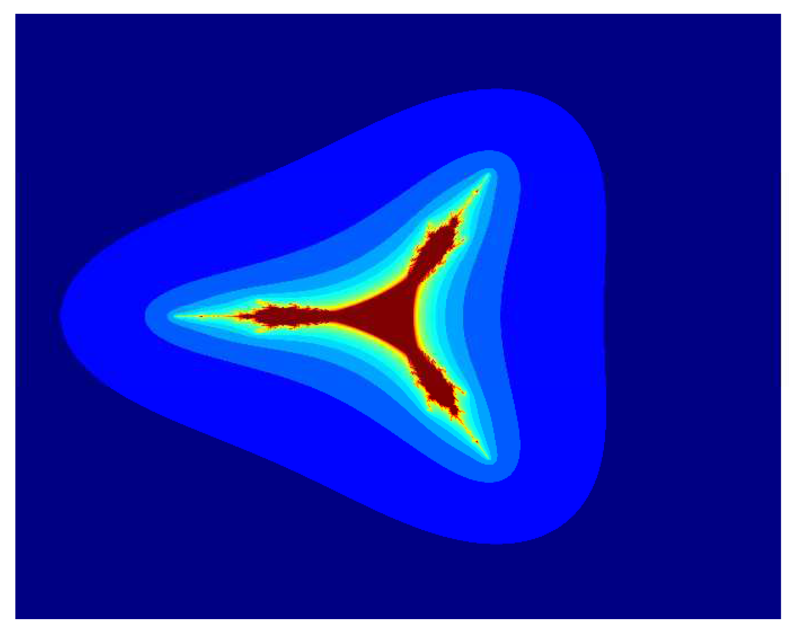
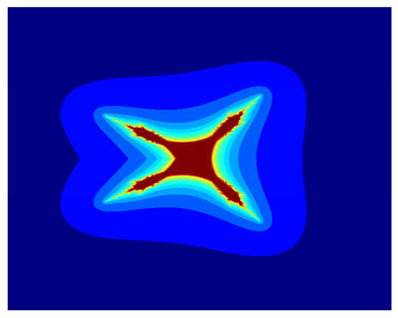
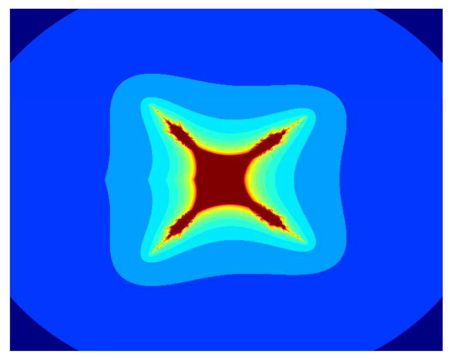
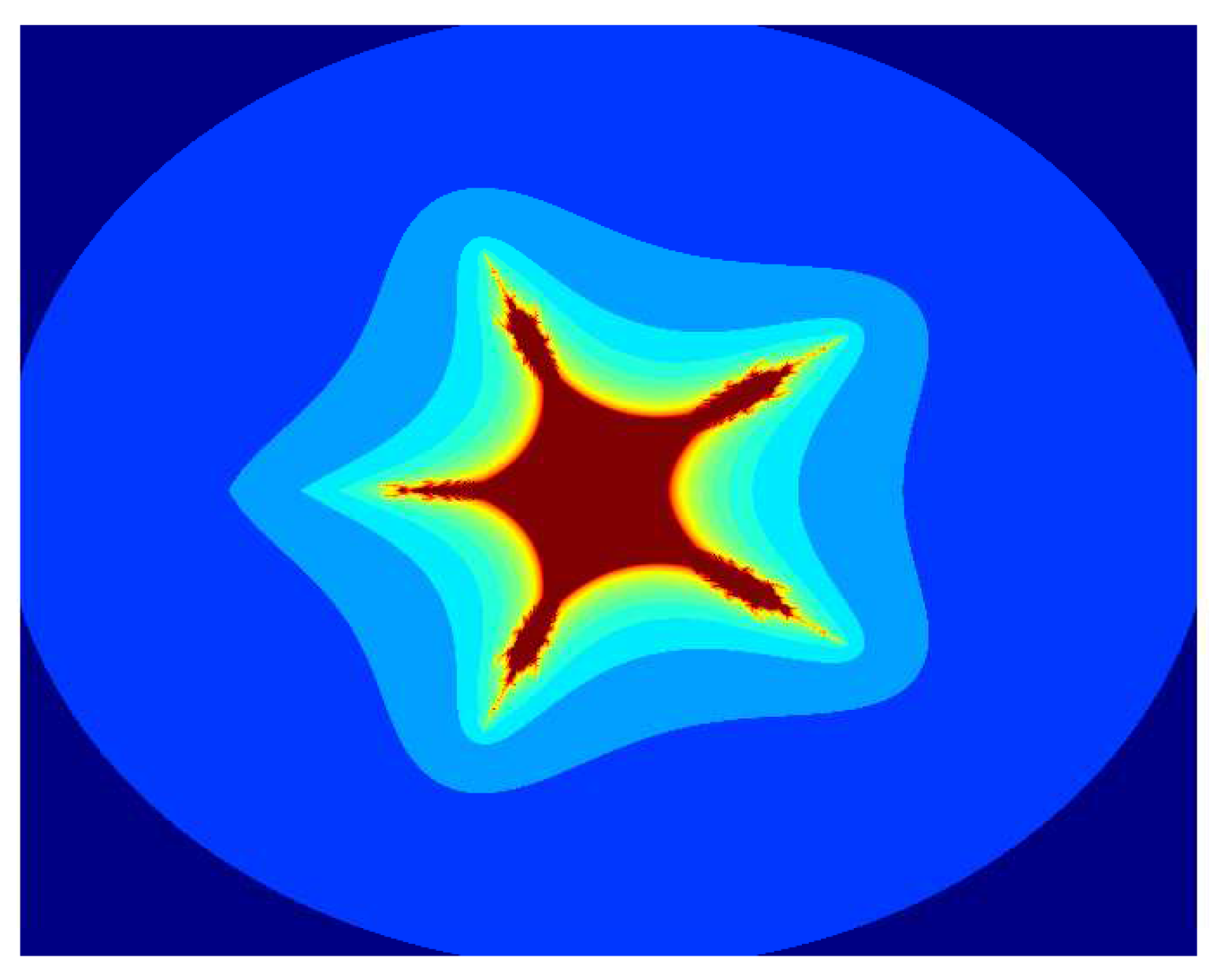
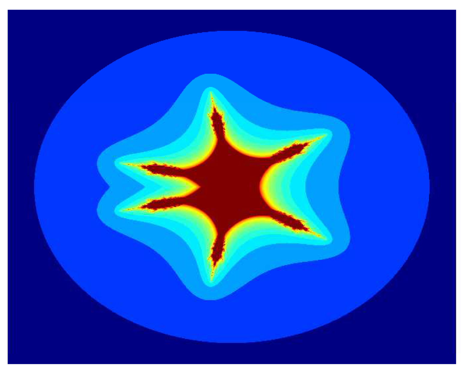
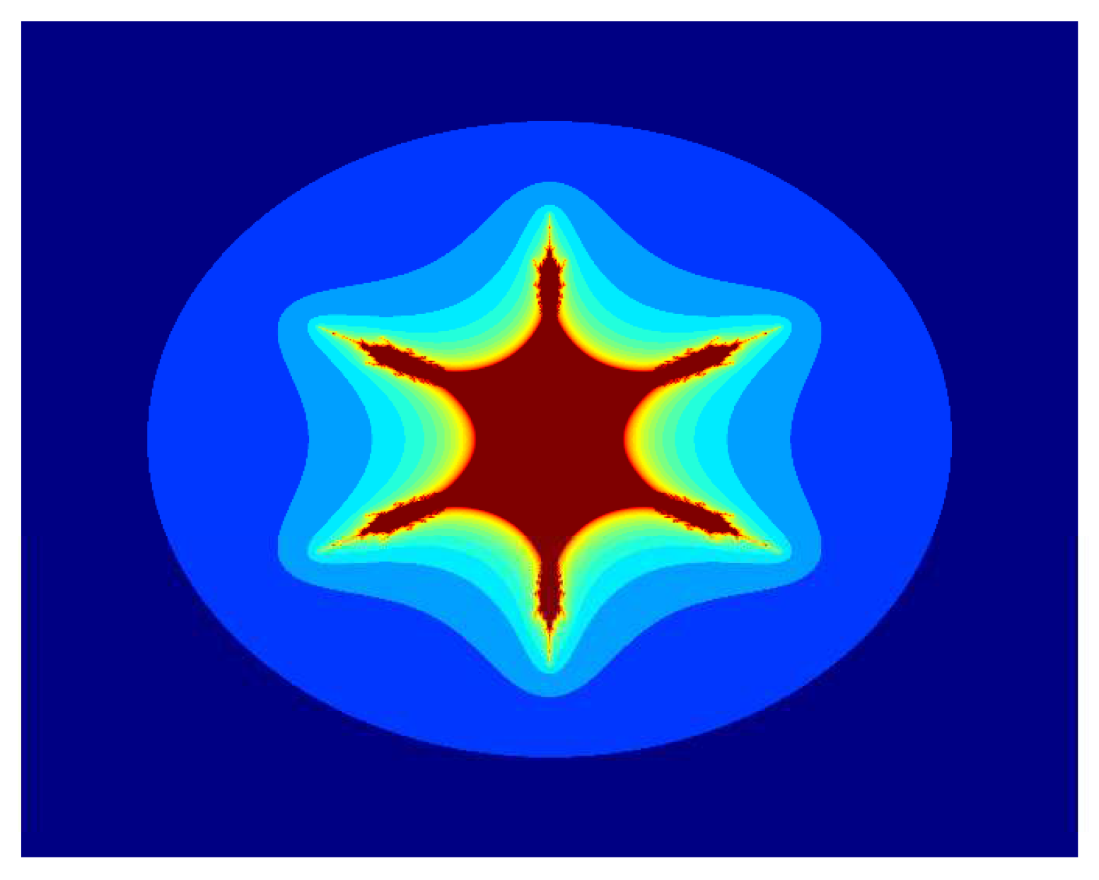
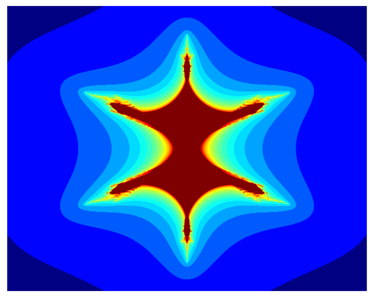
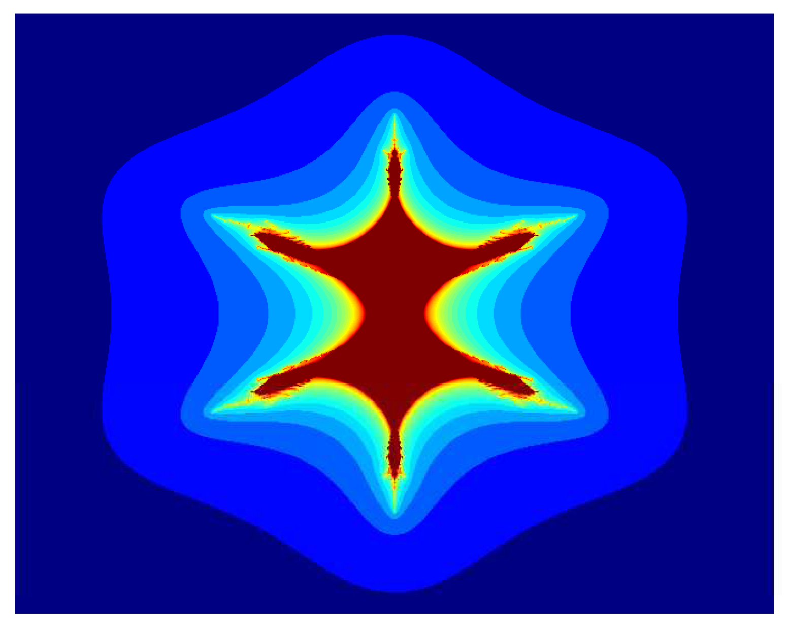
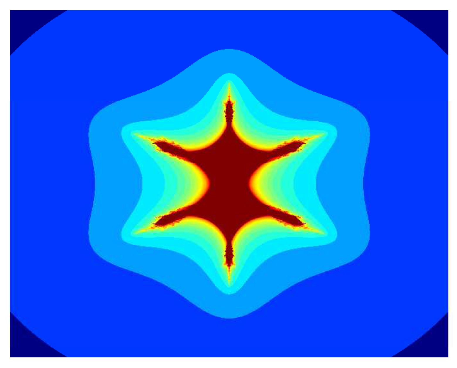
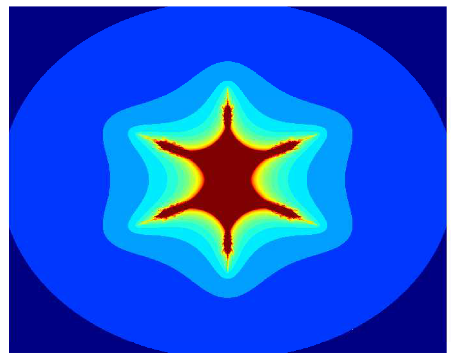
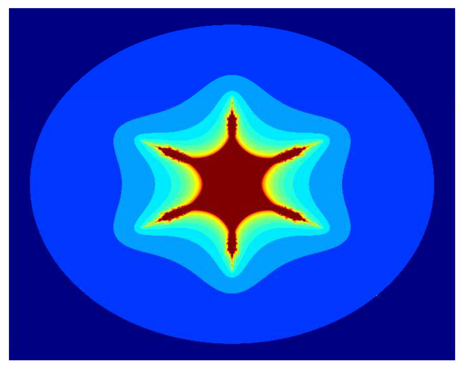
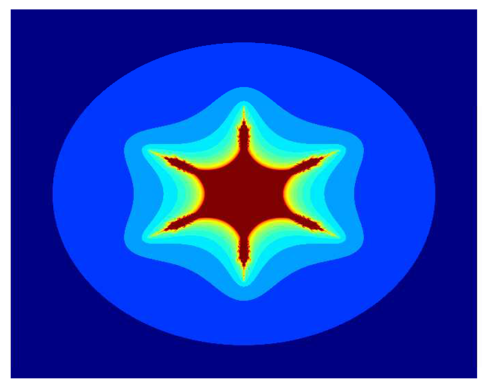
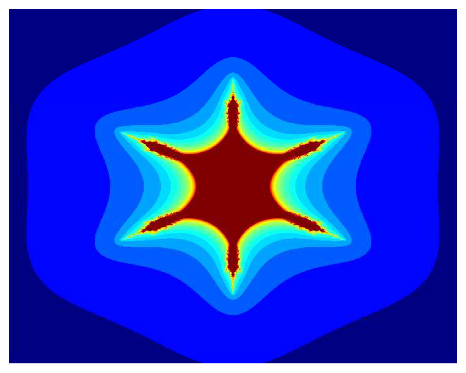
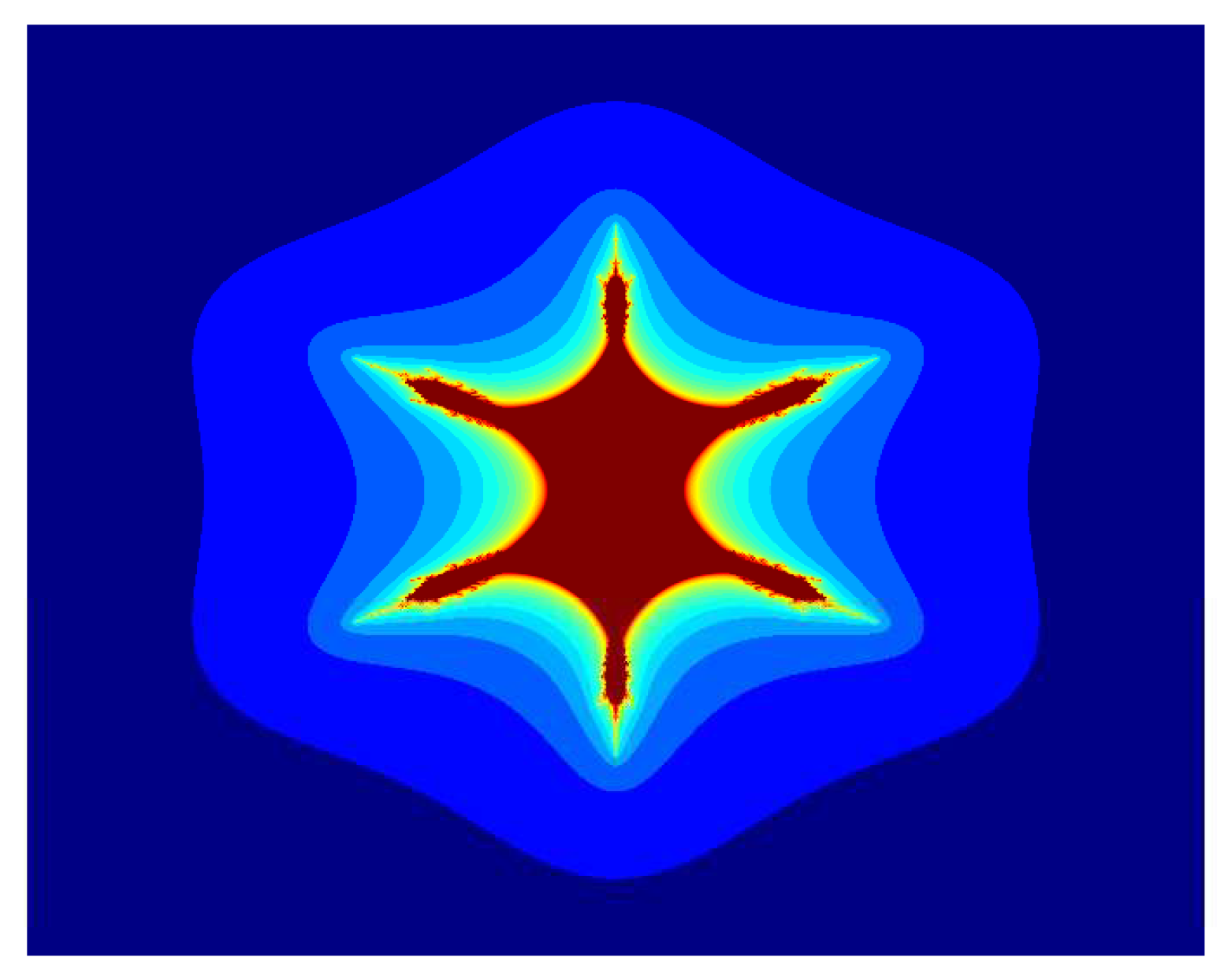
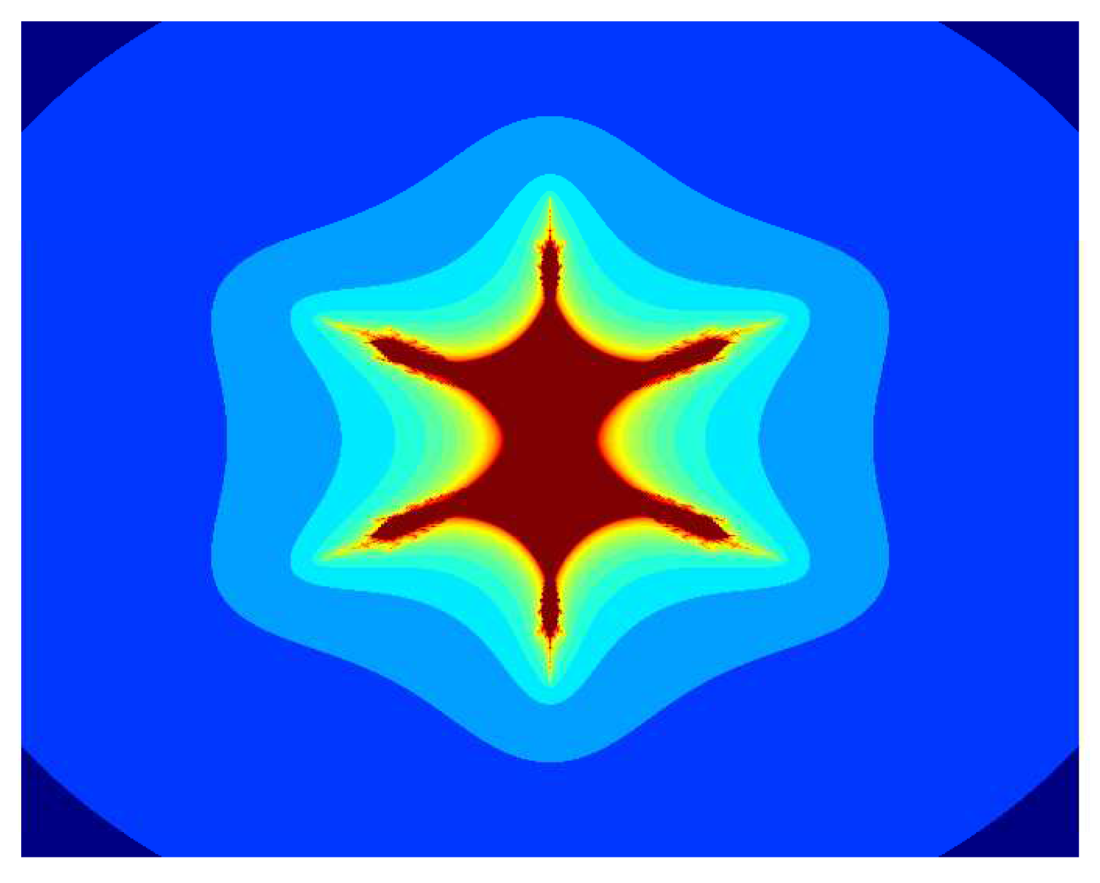
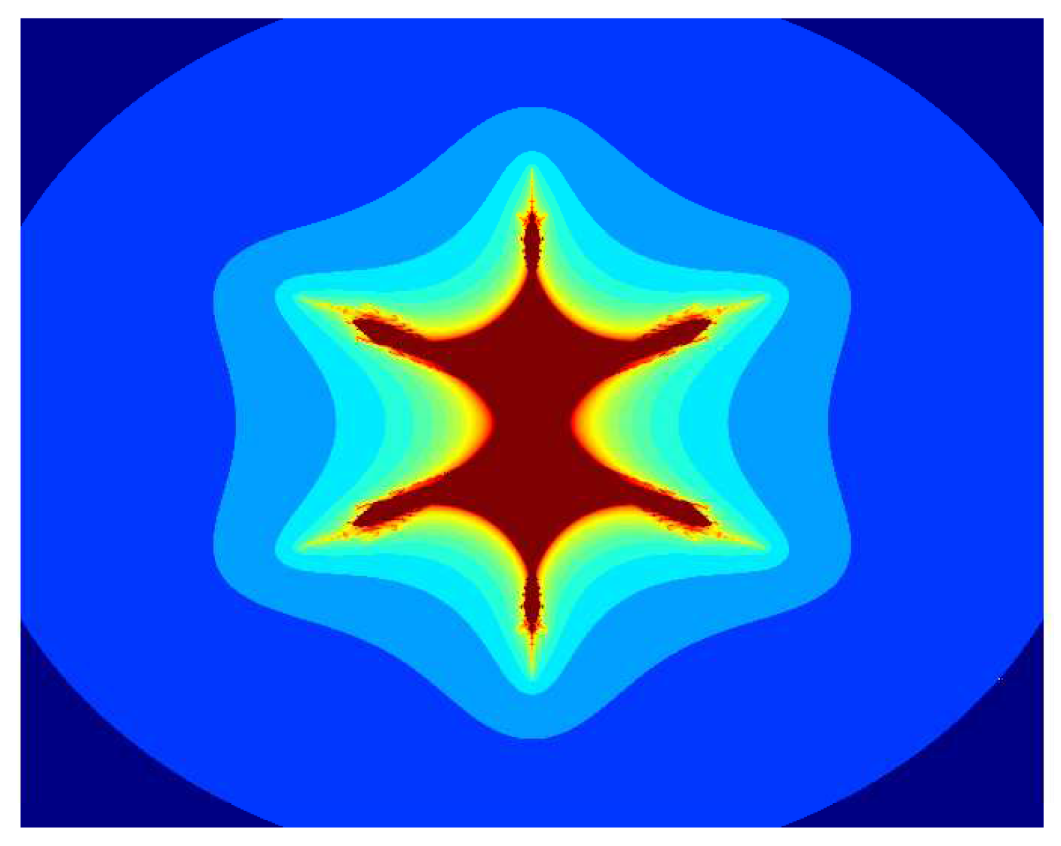
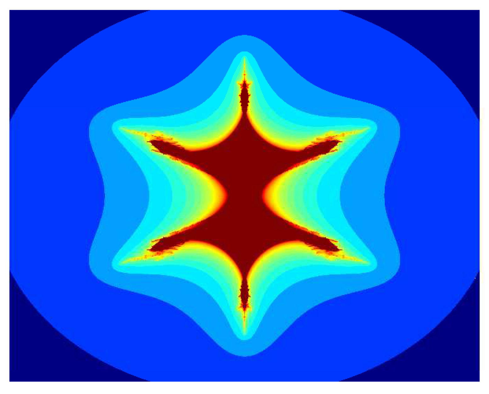
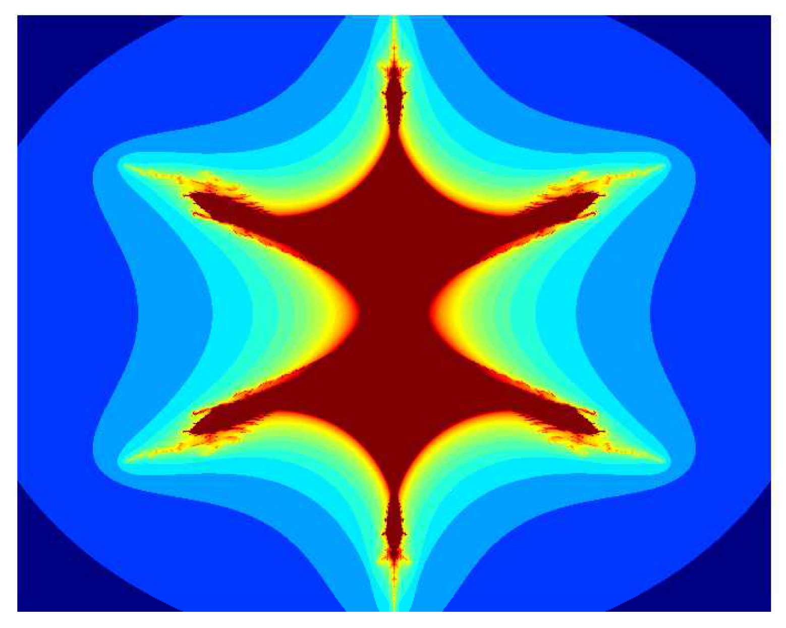
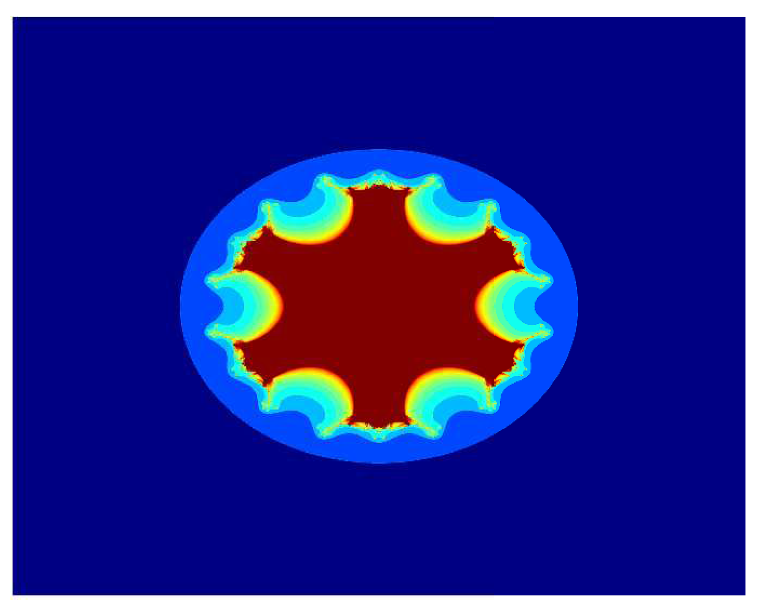
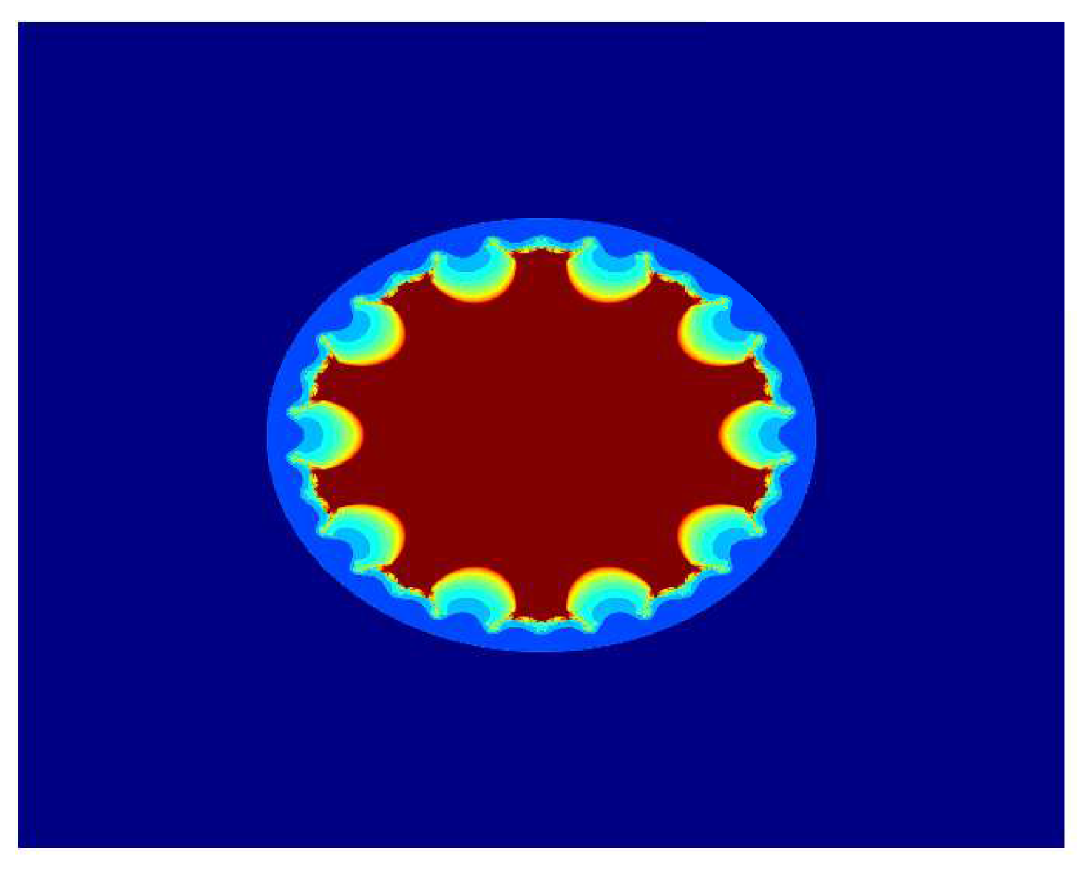
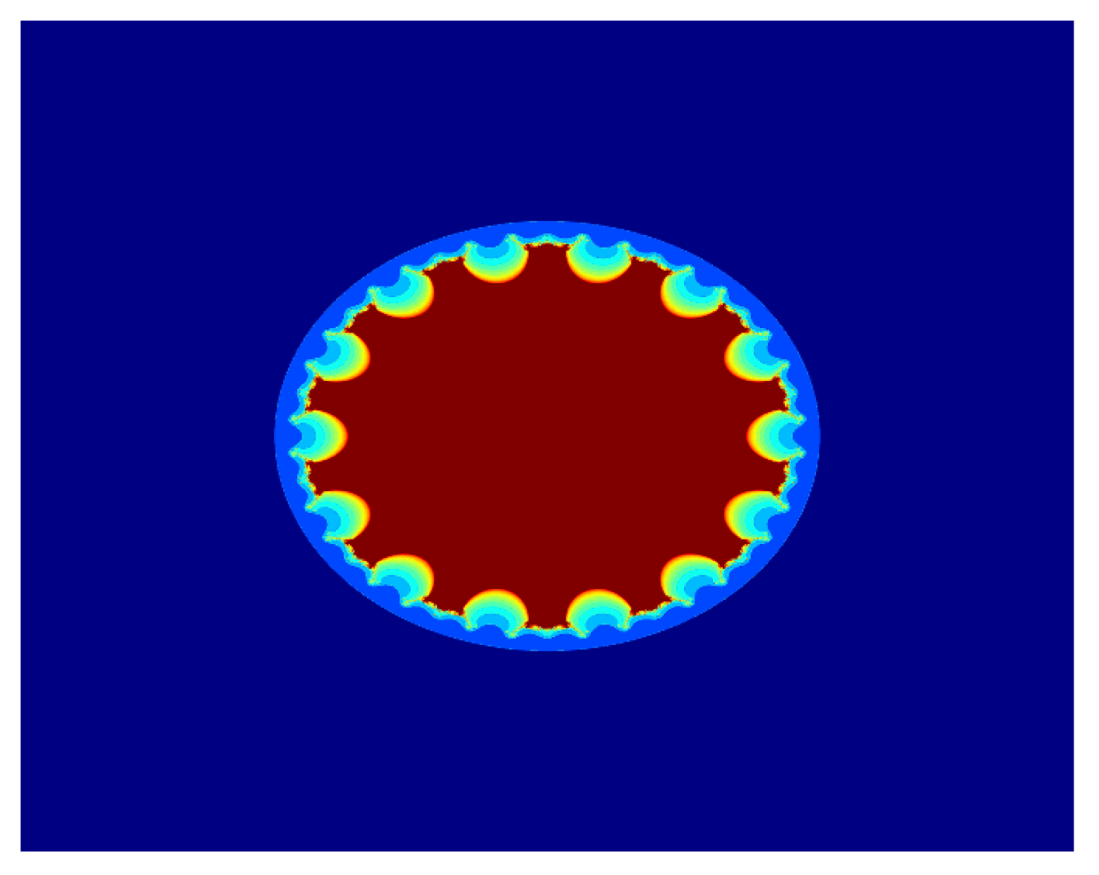
4. Graphical Examples

In this study, we present some multicorn sets of τ c ( z ) = z ¯ k + c m , where k 2 , c 0 C , and m R , by using S-iteration with h-convexity. The proposed criterion is used in an escape time algorithm [23] and implemented in MATLAB R2013a to generate the graphics.
In all graphical examples, we fix A = [ 2 , 2 ] 2 as the area for multicorn sets and k = 50 as the maximum number of iteration.
Now we discuss the dynamical behaviour of z ¯ k + c m by using the proposed iteration for k = 2 , a = 0.85 , a = 0.75 and varying the function parameter m. Image ( a ) in Figure 1 is a tricorn set, and the remaining images in Figure 2, Figure 3, Figure 4, Figure 5 and Figure 6 are multicorn sets. We observe that as we increase the value of m from 1 to 2, the average image execution time of all images in Figure 1, Figure 2, Figure 3, Figure 4, Figure 5 and Figure 6 increases from 11.05 s to  22.47 s. Additionally, the number of corns on the main body of images increases by m times k + 1 .
In Figure 7, Figure 8, Figure 9, Figure 10, Figure 11 and Figure 12, we fix k = 2 , a = 0.5 , and m = 2 and vary parameter a in the S-iteration with h-convexity orbit. We see in Figure 7, Figure 8, Figure 9, Figure 10, Figure 11 and Figure 12 that 6 corns appeared on the main body of images, and the size of sets decreases as the parameter a increases. We notice that as we increase the values of a from 0.165 to 1, the average image execution time of all images in Figure 7, Figure 8, Figure 9, Figure 10, Figure 11 and Figure 12 decreases from 19.71 s to  10.12 s.
Similarly, for k = 2 , a = 0.5 , m = 2 , and varying parameter a in the S-iteration with h-convexity orbit, the images in Figure 13, Figure 14, Figure 15, Figure 16, Figure 17 and Figure 18 have 6 corns on the main body of images, and the size of sets also decreases as the parameter a increases. Again, we notice that as we increase the values of a from 0.165 to 1, the average image execution time of all images in Figure 13, Figure 14, Figure 15, Figure 16, Figure 17 and Figure 18 decreases from 21.29 s to  11.51  s.
The last three Figure 19, Figure 20 and Figure 21 have the images for k = 5 , a = 0.5 , a = 0.5 , and varying parameter m in the S-iteration with h-convexity orbit.

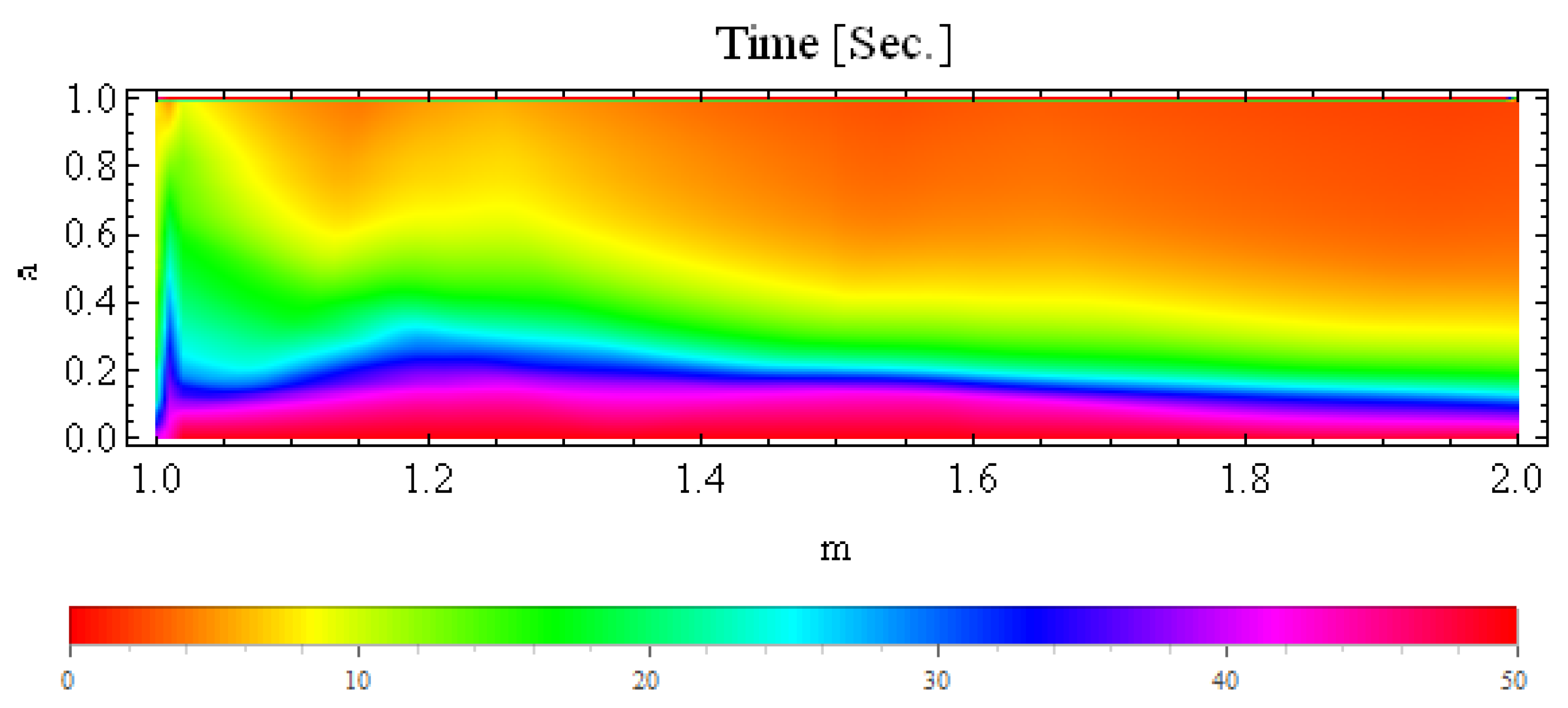
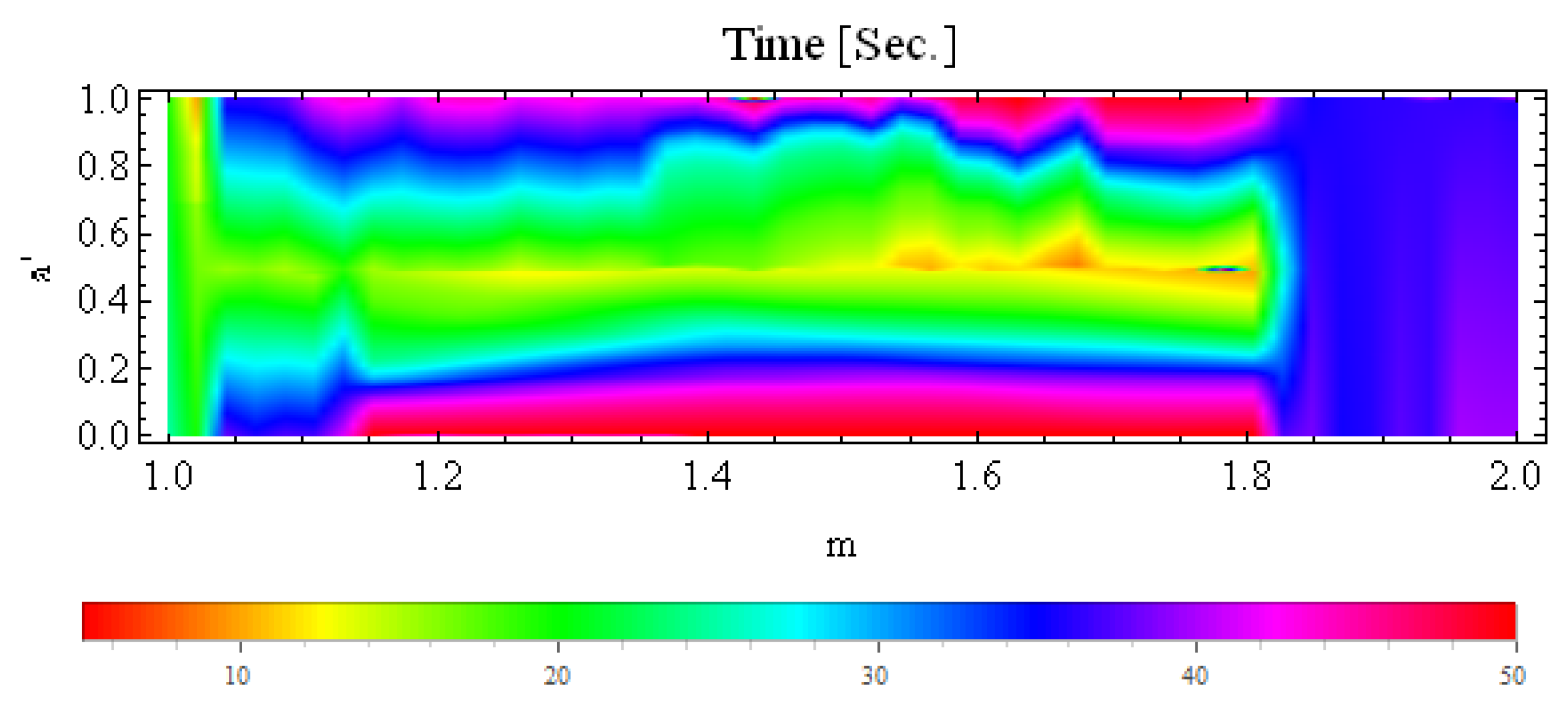
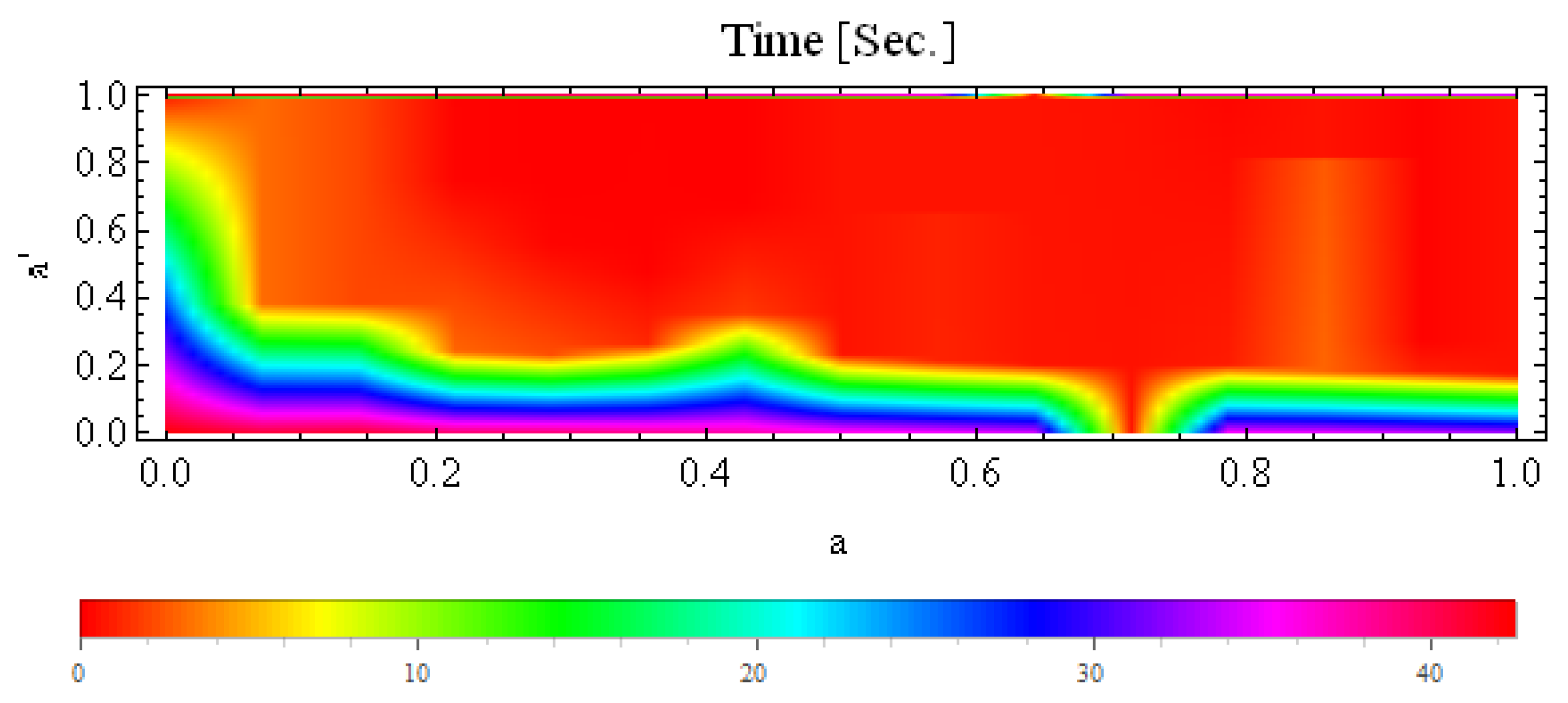
5. Numerical Simulations and Discussion

Analysing dependency between multicorn sets and the iteration input parameters is very complex. See, for example, [22,24,25], wherein the authors present the dependency via numerical measures.
In Section 4, we studied the graphs of multicorn sets by using the ETA (i.e., escape time algorithm). In this section, we study the average image execution time variation by varying the pairs of parameters ( a , m ) , ( a , m ) , and ( a , a ) . We fix a and the number of iterations for pair ( a , m ) , a and the number of iterations for pair ( a , m ) , and m and the number of iterations for pair ( a , a ) , respectively.
In the first numerical case, we use the parameters a and m in the form of intervals as follow:
  • ( 0 , 1 ] for a;
  • [ 1 , 2 ) for m.
For each interval, we calculate 100 values for a and 100 for m by using 0.01 as the step size. All calculations and graphs were analysed on a computer with specifications: Intel(R) Core(TM) i5-3320M (@ 2.60 GHz), 4 GB RAM, and 64-bit Windows 10. To calculate average image execution time, we implemented the algorithm in Mathematica. The image resolution was adjusted to 800 × 800 pixels in the Mathematica code. To analyse the behavioural effect of input parameters a and m on multicorn sets in the S-iteration with h-convexity orbit, we fix a = 0.5 , and the number of iterations is equal to 15. The colour map of the times is bounded in the time values [ 8.26 s, 49.90 s].
The graph for k = 2 is presented in Figure 22 for the S-iteration with h-convexity. In this graph, we observe that the algorithm took the maximum time to execute the image at a = 0.09 and m = 1.23 and the minimum time at a = 1 and m = 1.99 . We also observe that the algorithm took the maximum time for every value of m and a ( 0 , 0.2 ) , as we can see in Figure 22 as the pink and dark-red coloured area.
In the second numerical case, we use the parameters a and m in the form of intervals as follow:
  • ( 0 , 1 ] for a ,
  • [ 1 , 2 ) for m.
For each interval, we calculate 100 values for a and 100 for m by using 0.01 as the step size. To analyse the behavioural effect of input parameters a and m on multicorn sets in the S-iteration with h-convexity orbit, we fix a = 0.7 , and the number of iterations is equal to 15. The colour map of the times is bounded in the time values [ 4.53 s, 50 s].
The graph for k = 2 is presented in Figure 23 for the S-iteration with h-convexity. In this graph, we observe that the algorithm took the maximum time to execute the images when a ( 0 , 0.15 ) and m ( 1.65 , 1.817 ) and the minimum time at a = 1 and m = 1.99 (i.e., 4.53 s). From the graph in Figure 23, we make the following observations:
  • For a ( 0 , 1 ] ) and m ( 1 , 1.06 ) , image execution times belong to (13 s, 15 s);
  • For a ( 0.2 , 0.9 ] and m ( 1 , 1.8 ) , image execution times belong to (10 s, 30 s);
  • For a ( 0.1 , 0.18 ] and m ( 1.17 , 1.8 ) , image execution times belong to (38 s, 50 s];
  • For a ( 0 , 1 ] and m ( 1.8 , 1.99 ] , image execution times belong to (27 s, 34 s);
  • For a ( 0.87 , 1 ] and m ( 1.17 , 1.8 ] , image execution times belong to (30 s, 50 s].
In the second numerical case, we use the parameters a and m in the form of intervals as follow:
  • ( 0 , 1 ] for a ,
  • ( 0 , 1 ] for m.
For each interval, we calculate 100 values for a and 100 for a , by using 0.01 as the step size. To analyse the behavioural effect of input parameters a and a on multicorn sets in the S-iteration with h-convexity orbit, we fix m = 3 , and the number of iterations is equal to 15. The colour map of the times is bounded in the time values [ 0.013 s, 42.573 s].
The graph for k = 2 is presented in Figure 24 for the S-iteration with h-convexity. In this graph, we observe that the algorithm took the maximum time to execute the images when a = 0.01 and a = 0.01 (i.e., 42.573 s) and the minimum time at a = 0.72 and a = 1 (i.e., 0.013 s). From the graph in Figure 23, we make the following observations:
  • For a ( 0 , 0.18 ] ) and a ( 0 , 0.63 ) , image execution times belong to (30 s, 42.573 s];
  • For a ( 0.2 , 1 ] and a ( 0.08 , 1 ] , image execution times belong to [0.013 s, 3.87 s).
In the above discussion, we notice that the graph in Figure 23 is very difficult to analyse as compared to the graphs in Figure 22 and Figure 24 because the pair ( a , t ) attained highest and lowest values at different points, whereas the highest and lowest time values for pairs ( a , m ) and ( a , a ) are easy to see in the graphs of Figure 22 and Figure 24.

6. Conclusions

In this study, we presented the escape criterion of the conjugate complex function τ c ( z ) = z ¯ k + c m , where k 2 , c 0 C , and m R , by using S-iteration with h-convexity, and we developed an escape criterion of the proposed function for S-iteration with h-convexity. By using the developed escape criterion in the escape time Algorithm 1, we generated a variety of multicorn sets. We observed that for m N , images consist of m ( k + 1 ) -corns. The iteration parameters a and a have a huge effect on the size of multicorn sets, i.e., the larger the values of iteration parameters a and a are, the bigger the set is. Moreover, we calculated the average time of image execution in seconds for the pairs ( a , m ) , ( a , m ) , and ( a , a ) by using S-iteration with h-convexity. The numerical simulations showed that the variations in pairs ( a , m ) , ( a , m ) , and ( a , a ) drastically affect the image generation time.
Moreover, T ( z , α , τ ) , T ( z , α , β , τ ) , and T ( z , α , β , γ , τ ) are commonly used maps in the literature, but for future research, the authors may focus on the utilization of other maps such as T ( z , α , τ n ) , T ( z , α , β , τ n ) , and T ( z , α , β , γ , τ n ) with iterations of single-, double-, and triple-step feedbacks. One more future direction for studying fractals via fixed-point iterations could be the utilization of transcendental functions by replacing the complex parameter c.
More recently, the use of different spline methods and fractional differential equations is remarkable [26]. Spline methods and functions are also applied in fractals to visualise the data [27]. Therefore, one can study different spline methods and functions to investigate fractal patterns.
We anticipate that the results of this study will inspire individuals who have an interest in automatically producing beautiful graphics.
Algorithm 1 Multicorn set generation
Fractalfract 07 00486 i001

Author Contributions

Conceptualization, A.T., M.T. and R.S.; Data curation, K.I., M.A. and K.S.; Formal analysis, A.T., M.T., M.A. and K.S.; Investigation, A.T. and M.T.; Methodology, A.T., M.T. and M.A.; Project administration, K.S. and R.S; Resources, K.S.; Supervision, K.I; Validation, M.T. and R.S; Writing—review and editing, M.T. and M.A. All authors have read and agreed to the published version of the manuscript.

Funding

This research was funded by the Deanship of Scientific Research at Majmaah University for supporting this work under Project Number No. R-2023-477.

Data Availability Statement

The research is theoretical in nature. As a result, no data were used.

Acknowledgments

Asifa Tassaddiq would like to thank the Deanship of Scientific Research at Majmaah University for supporting this work under Project Number No. R-2023-477. The authors are also thankful to the worthy reviewers and editors for their useful and valuable suggestions for improving this paper, which led to a better presentation.

Conflicts of Interest

The authors declare no conflict of interest.

References

  1. Taylor, R.P. The Potential of Biophilic Fractal Designs to Promote Health and Performance: A Review of Experiments and Applications. Sustainability 2021, 13, 823. [Google Scholar] [CrossRef]
  2. Srivastava, H.M.; Saad, K.M.; Hamanah, W.M. Certain new models of the multi-space fractal-fractional Kuramoto-Sivashinsky and Korteweg-de Vries equations. Mathematics 2022, 10, 1089. [Google Scholar] [CrossRef]
  3. Kumar, S. Public Key Cryptographic System Using Mandelbrot Sets. In Proceedings of the MILCOM 2006–2006 IEEE Military Communications Conference, Washington, DC, USA, 23–25 October 2006; pp. 1–5. [Google Scholar]
  4. Zhang, X.; Wang, L.; Zhou, Z.; Niu, Y. A chaos-based image encryption technique utilizing Hilbert curves and H-Fractals. IEEE Access 2019, 7, 74734–74746. [Google Scholar] [CrossRef]
  5. Sun, Y.; Chen, L.; Xu, R.; Kong, R. An image encryption algorithm utilizing Julia sets and Hilbert curves. PLoS ONE 2014, 9, e84655. [Google Scholar] [CrossRef] [PubMed]
  6. Fisher, Y. Fractal image compression. Fractals 1994, 2, 347–361. [Google Scholar] [CrossRef] [Green Version]
  7. Liu, S.-A.; Bai, W.-L.; Liu, G.-C.; Li, W.-H.; Srivastava, H.M. Parallel fractal compression method for big video data. Complexity 2018, 2018, 2016976. [Google Scholar] [CrossRef] [Green Version]
  8. Liu, S.-A.; Xu, X.-Y.; Srivastava, G.; Srivastava, H.M. Fractal properties of the generalized Mandelbrot set with complex exponent. Fractals 2023, 31, 0218-348X. [Google Scholar] [CrossRef]
  9. Tassaddiq, A. General escape criteria for the generation of fractals in extended Jungck–Noor orbit. Math. Comput. Simul. 2022, 196, 1–14. [Google Scholar] [CrossRef]
  10. Barnsley, M. Fractals Everywhere; Academic: Boston, MA, USA, 1993. [Google Scholar]
  11. Mandelbrot, B.B. The Fractal Geometry Nature; Freeman: New York, NY, USA, 1982; Volume 2. [Google Scholar]
  12. Lakhtakia, A.; Varadan, W.; Messier, R.; Varadan, V.K. On the symmetries of the Julia sets for the process zp + c. J. Phys. A Math. Gen. 1987, 20, 3533–3535. [Google Scholar] [CrossRef]
  13. Blanchard, P.; Devaney, R.L.; Garijo, A.; Russell, E.D. A generalized version of the Mcmullen domain. Int. J. Bifurc. Chaos 2008, 18, 2309–2318. [Google Scholar] [CrossRef] [Green Version]
  14. Crowe, W.D.; Hasson, R.; Rippon, P.J.; Strain-Clark, P.E.D. On the structure of the Mandelbar set. Nonlinearity 1989, 2, 541. [Google Scholar] [CrossRef]
  15. Milnor, J.W. Dynamics in one complex variable Introductory lectures. arXiv 1990, arXiv:math/9201272. [Google Scholar]
  16. Alexander, C.; Giblin, I.; Newton, D. Symmetry groups of fractals. Math. Intell. 1992, 14, 32–38. [Google Scholar] [CrossRef]
  17. Lau, E.; Schleicher, D. Symmetries of fractals revisited. Math. Intell. 1996, 18, 45–51. [Google Scholar] [CrossRef]
  18. Nakane, S.; Schleicher, D. On multicorns and unicorns i: Antiholomorphic dynamics, hyperbolic components and real cubic polynomials. Int. J. Bifurc. Chaos 2003, 13, 2825–2844. [Google Scholar] [CrossRef] [Green Version]
  19. Devaney, R. A First Course in Chaotic Dynamical Systems. In Theory and Experiment; Addison-Wesley: New York, NY, USA, 1992. [Google Scholar]
  20. Liu, X.; Zhu, Z.; Wang, G.; Zhu, W. Composed accelerated escape time algorithm to construct the general Mandelbrot sets. Fractals 2001, 9, 149–153. [Google Scholar] [CrossRef]
  21. Kang, S.M.; Rafiq, A.; Latif, A.; Shahid, A.A.; Kwun, Y.C. Tricorns and multicorns of S-iteration scheme. J. Function Spaces 2015, 2015, 417167. [Google Scholar] [CrossRef] [Green Version]
  22. Tanveer, M.; Nazeer, W.; Gdawiec, K. On the Mandelbrot set of zp + logct via the Mann and Picard–Mann iterations. In Mathematics and Computers in Simulation; Elsevier: Amsterdam, The Netherlands, 2023; Volume 209, pp. 184–204. [Google Scholar]
  23. Barrallo, J.; Jones, D.M. Coloring Algorithms for Dynamical Systems in the Complex Plane. In Visual Mathematics; Mathematical Institute SASA: Belgrade, Serbia, 1999; Volume 4, no. 4. [Google Scholar]
  24. Kumari, S.; Gdawiec, K.; Nandal, A.; Postolache, M.; Chugh, R. A Novel Approach to Generate Mandelbrot Sets, Julia Sets and Biomorphs via Viscosity Approximation Method. Chaos Solitons Fractals 2022, 163, 112540. [Google Scholar] [CrossRef]
  25. Shahid, A.A.; Nazeer, W.; Gdawiec, K. The Picard–Mann Iteration with s-convexity in the Generation of Mandelbrot and Julia Sets. Monatshefte Math. 2021, 195, 565–585. [Google Scholar] [CrossRef]
  26. Qiao, L.; Xu, D. A fast ADI orthogonal spline collocation method with graded meshes for the two-dimensional fractional integro-differential equation. Adv. Comput. Math. 2021, 47, 64. [Google Scholar] [CrossRef]
  27. Katiyar, S.K.; Chand, A.B.; Kumar, G.S. A new class of rational cubic spline fractal interpolation function and its constrained aspects. Appl. Math. Comput. 2019, 346, 319–335. [Google Scholar] [CrossRef]
Figure 1. Multicorn sets for k = 2 , a = 0.65 , a = 0.75 , and parameter m = 1 in the S-iteration with h-convexity orbit.
Fractalfract 07 00486 g001
Figure 2. Multicorn sets for k = 2 , a = 0.65 , a = 0.75 , and parameter m = 1.2 in the S-iteration with h-convexity orbit.
Fractalfract 07 00486 g002
Figure 3. Multicorn sets for k = 2 , a = 0.65 , a = 0.75 , and parameter m = 1.4 in the S-iteration with h-convexity orbit.
Fractalfract 07 00486 g003
Figure 4. Multicorn sets for k = 2 , a = 0.85 , a = 0.75 , and parameter m = 1.6 in the S-iteration with h-convexity orbit.
Fractalfract 07 00486 g004
Figure 5. Multicorn sets for k = 2 , a = 0.85 , a = 0.75 , and parameter m = 1.8 in the S-iteration with h-convexity orbit.
Fractalfract 07 00486 g005
Figure 6. Multicorn sets for k = 2 , a = 0.85 , a = 0.75 , and parameter m = 2 in the S-iteration with h-convexity orbit.
Fractalfract 07 00486 g006
Figure 7. Multicorn sets for k = 2 , a , = 0.5 , m = 2 , and parameter a = 0.165 in the S-iteration with h-convexity orbit.
Fractalfract 07 00486 g007
Figure 8. Multicorn sets for k = 2 , a , = 0.5 , m = 2 , and parameter a = 0.33 in the S-iteration with h-convexity orbit.
Fractalfract 07 00486 g008
Figure 9. Multicorn sets for k = 2 , a , = 0.5 , m = 2 , and parameter a = 0.495 in the S-iteration with h-convexity orbit.
Fractalfract 07 00486 g009
Figure 10. Multicorn sets for k = 2 , a , = 0.5 , m = 2 , and parameter a = 0.66 in the S-iteration with h-convexity orbit.
Fractalfract 07 00486 g010
Figure 11. Multicorn sets for k = 2 , a , = 0.5 , m = 2 , and parameter a = 0.825 in the S-iteration with h-convexity orbit.
Fractalfract 07 00486 g011
Figure 12. Multicorn sets for k = 2 , a , = 0.5 , m = 2 , and parameter a = 0.99 in the S-iteration with h-convexity orbit.
Fractalfract 07 00486 g012
Figure 13. Multicorn sets for k = 2 , a = 0.5 , m = 2 , and parameter a = 0.165 in the S-iteration with h-convexity orbit.
Fractalfract 07 00486 g013
Figure 14. Multicorn sets for k = 2 , a = 0.5 , m = 2 , and parameter a = 0.33 in the S-iteration with h-convexity orbit.
Fractalfract 07 00486 g014
Figure 15. Multicorn sets for k = 2 , a = 0.5 , m = 2 , and parameter a = 0.495 in the S-iteration with h-convexity orbit.
Fractalfract 07 00486 g015
Figure 16. Multicorn sets for k = 2 , a = 0.5 , m = 2 , and parameter a = 0.66 in the S-iteration with h-convexity orbit.
Fractalfract 07 00486 g016
Figure 17. Multicorn sets for k = 2 , a = 0.5 , m = 2 , and parameter a = 0.825 in the S-iteration with h-convexity orbit.
Fractalfract 07 00486 g017
Figure 18. Multicorn sets for k = 2 , a = 0.5 , m = 2 , and parameter a = 0.99 in the S-iteration with h-convexity orbit.
Fractalfract 07 00486 g018
Figure 19. Multicorn sets for k = 5 , a = 0.5 , a = 0.5 , and parameter m = 3 in the S-iteration with h-convexity orbit; execution time = 25.85 s.
Fractalfract 07 00486 g019
Figure 20. Multicorn sets for k = 5 , a = 0.5 , a = 0.5 , and parameter m = 5 in the S-iteration with h-convexity orbit; execution time = 40.12 .
Fractalfract 07 00486 g020
Figure 21. Multicorn sets for k = 5 , a = 0.5 , a = 0.5 , parameter m = 7 in the S-iteration with h-convexity orbit; execution time = 44.48 s.
Fractalfract 07 00486 g021
Figure 22. Plot of average time (in seconds) between a and m for multicorn set generated in the S-iteration with h-convexity orbit.
Fractalfract 07 00486 g022
Figure 23. Plot of the average time (in seconds) between a and m for multicorn sets generated in the S-iteration with h-convexity orbit.
Fractalfract 07 00486 g023
Figure 24. Plot of the average time (in seconds) between a and a for multicorn set generated in the S-iteration with h-convexity orbit.
Fractalfract 07 00486 g024
Disclaimer/Publisher’s Note: The statements, opinions and data contained in all publications are solely those of the individual author(s) and contributor(s) and not of MDPI and/or the editor(s). MDPI and/or the editor(s) disclaim responsibility for any injury to people or property resulting from any ideas, methods, instructions or products referred to in the content.

