
On a Quadratic Nonlinear Fractional Equation

1
CITMAga, Universidade de Vigo, Departamento de Matemática Aplicada II, E.E. Aeronáutica e do Espazo, Campus As Lagoas-Ourense, 32004 Ourense, Spain
2
CITMAga, Universidade de Santiago de Compostela, 15782 Santiago de Compostela, Spain
*
Author to whom correspondence should be addressed.
Fractal Fract. 2023, 7(6), 469; https://doi.org/10.3390/fractalfract7060469
Submission received: 15 April 2023
/
Revised: 5 June 2023
/
Accepted: 6 June 2023
/
Published: 12 June 2023
(This article belongs to the Special Issue Operators of Fractional Calculus and Their Multidisciplinary Applications, 2nd Edition)
Abstract
:In this paper, we study a quadratic nonlinear equation from the fractional point of view. An explicit solution is given in terms of the Lambert special function. A new phenomenon appears involving the collapsing of the solution and the blow-up of the derivative. The explicit representation of the solution reveals the non-elementary nature of the solution.
Keywords:
logistic ordinary differential equation; blow-up; fractional differential equation; Lambert function; non-elementary functions; non-uniquenessMSC:
34A05; 34A34; 34M501. Introduction
In logistic population growth, the concept of environmental carrying capacity is modelled by the classical logistic ordinary differential equation [1]:
The Richards ordinary differential equation is a generalization of the above logistic differential equation by introducing a new parameter, :
The latter equation can be explicitly solved
and for it gives the solution of the logistic differential Equation (1). We note that the exponential term in the Richards equation has a one-to-one nonlinear correspondence with the basic reproduction number of the SIR (susceptible–infectious–recovered) compartmental epidemiological model [2]. Recently, some researchers have discovered the connection of the Richards model to the epidemic dynamics of COVID-19 [3,4].
For , we have already considered the logistic fractional differential equation (see e.g., [5])
as well as the fractional Richards differential equation for ,
The fractional Richards equation has been considered in very few articles. For example, it has been considered for water transport [6], but has only been approximated numerically or using peridynamic theory as in [7]. It therefore seems of interest to study the more general nonlinear fractional differential equation
This is our main motivation in this brief report. We point out that even simple nonlinear equations such as the Caputo fractional logistic equation have no analytical known solution.
For some general references on fractional differential equations and their applications, refer to [8]. If represents the Caputo–Fabrizio fractional derivative [9], then integrating by using the Losada–Nieto fractional integral we obtain
Thus,
or equivalently
If, for an initial condition one has that
then the previous equation is equivalent, in a neighbourhood of to
with
In general, it is not possible to obtain an exact solution.
In this paper, we focus on the nonlinear fractional equation
For some biological applications, see [10]. Even for the solution of (2) is local. Indeed, for the initial condition , the solution is given by
and the right maximal interval of existence is .
Note that and then
If represents the Caputo–Fabrizio fractional derivative, then (2) is equivalent to
For an initial condition , we have to solve the equation
Integrating
For an initial condition , we can find the value of as
Then, (2) is equivalent to
Taking the exponential in both sides,
Setting
and
We observe that
that is, , being the Lambert function or product logarithm [11], for some integer k. This gives the solution x as
Using the value of the constant given in (4), one can finally write the solution to (2) in terms of the initial condition:
2. Example
Let us consider , . Then, the equation is
and the particular solution is given by
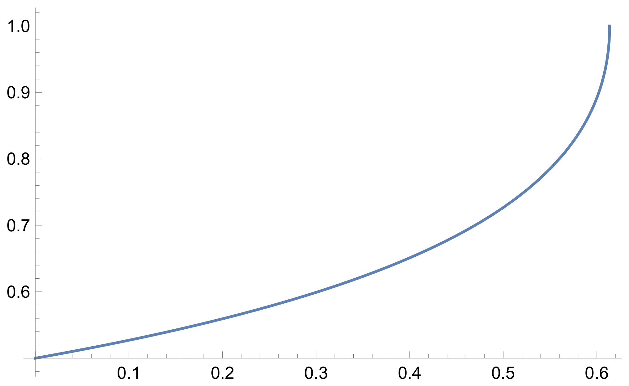
The solution exists locally. Noting that is positive for , it is increasing and blows up when x approaches (see Figure 1); that is,
To find the maximal interval of existence, we recall that the Lambert function is defined only for when Therefore, we have the condition
or
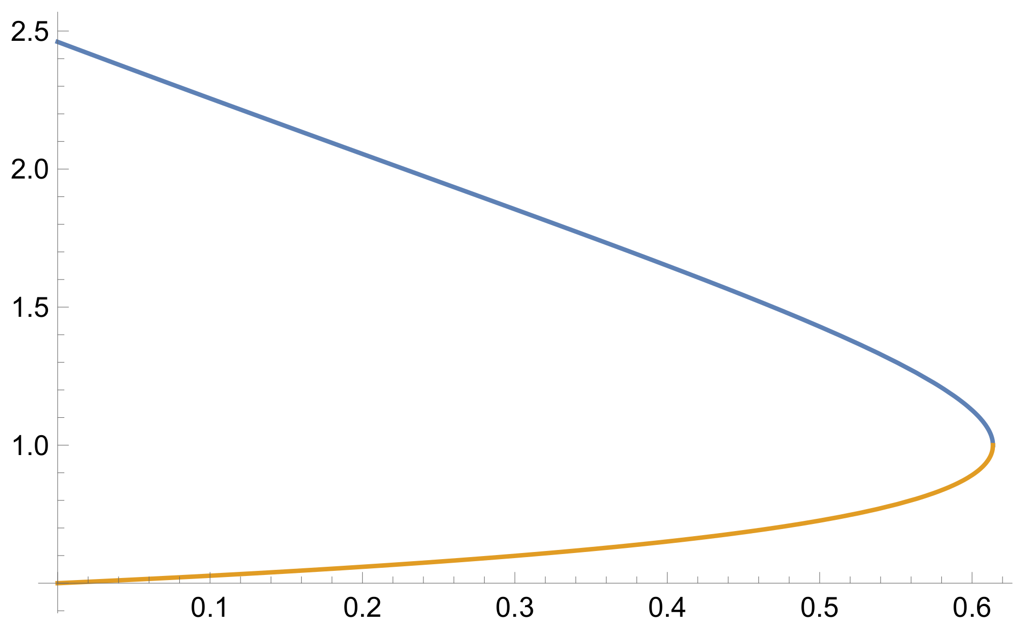
Observe that for the initial condition , and one cannot solve the differential equation. However, we can ask whether there exists a solution starting at that passes through that point . Such a solution is given by
Imposing the condition , we need
that is,
Therefore,
and (see Figure 2)
3. Lambert Function
Given a complex number z, we want to solve Equation (5). It has many solutions and hence it is a multivalued function. Thus, (5) is equivalent to
for some integer where is a branch of the inverse function . The principal branch is and denoted simply by .
The Lambert relation cannot be expressed in terms of elementary functions, i.e., it is non-elementary. In particular it is non-Liouvillian [12].
For , the equation has a single real solution given by and for we have two solutions: and For
The Lambert function satisfies the ordinary differential equation
Moreover,
with a radius of convergence equal to .
As another known but very relevant application of the Lambert function, let us compute the final population in the classical compartmental epidemic model [13,14]:
Here, as usual, S, I and R represent the susceptible, infectious and recovered population, respectively.
Recall that the basic reproduction number is the initial replacement number when just one infectious individual is introduced into a population of all susceptible individuals:
We have
Then,
and
This gives as the following function of
Taking the limit as
Equivalently,
and
Finally,
and
It is important to note that the solution I is a non-elementary function (see, for example, Theorem 10.3 in [14]).
We recall that an elementary function is defined as a function generated from a finite number of combinations and compositions of algebraic, exponential and logarithm functions under the four algebraic operations. A Liouvillian function is a function lying in some Liouvillian extension of for a constant field C.
Indeed, using the representation of S as a function of I through the Lambert function, it is possible to prove that the solution is not Liouvillian.
4. Conclusions
We have solved a fractional Richards differential equation.
New aspects of the methodology of solving it and the form of the solution are presented, and further research will be necessary to clearly reveal the complexity of nonlinear differential equations.
It will be of interest to explore fractional Richards differential equations in relation to the dynamics of epidemic compartmental models.
The dependence of the solution on the order of derivation would be of interest. The case when will be also contemplated.
Author Contributions
Conceptualization, J.J.N.; Methodology, I.A. and J.J.N.; Software, I.A. and J.J.N.; Validation, I.A.; Formal analysis, I.A. and J.J.N.; Investigation, I.A. and J.J.N.; Resources, I.A. and J.J.N.; Writing—original draft, I.A. and J.J.N.; Writing—review & editing, I.A. and J.J.N.; Project administration, J.J.N.; Funding acquisition, J.J.N. All authors have read and agreed to the published version of the manuscript.
Funding
This work has been partially supported by the Agencia Estatal de Investigación (AEI) of Spain under Grant PID2020-113275GB-I00, cofinanced by the European Community fund FEDER.
Conflicts of Interest
The authors declare that they have no known competing financial interest or personal relationships that could have appeared to influence the work reported in this paper.
References
- Area, I.; Nieto, J.J. Power series solution of the fractional logistic equation. Phys. A 2021, 573, 125947. [Google Scholar] [CrossRef]
- Wang, X.-S.; Wu, J.; Yang, Y. Richards model revisited: Validation by and application to infection dynamics. J. Theor. Biol. 2012, 313, 12–19. [Google Scholar] [CrossRef] [PubMed]
- Luo, X.; Duan, H.; Xu, K. A novel grey model based on traditional Richards model and its application in COVID-19. Chaos Solitons Fractals 2021, 142, 110480. [Google Scholar] [CrossRef] [PubMed]
- Smirnova, A.; Pidgeon, B.; Chowell, G.; Zhao, Y. The doubling time analysis for modified infectious disease Richards model with applications to COVID-19 pandemic. Math. Biosci. Eng. 2022, 19, 3242–3268. [Google Scholar] [CrossRef] [PubMed]
- Nieto, J.J. Solution of a fractional logistic ordinary differential equation. Appl. Math. Lett. 2022, 123, 107568. [Google Scholar] [CrossRef]
- Romashchenko, M.I.; Bohaienko, V.O.; Matiash, T.V.; Kovalchuk, V.P.; Krucheniuk, A.V. Numerical simulation of irrigation scheduling using fractional Richards equation. Irrig. Sci. 2021, 39, 385–396. [Google Scholar] [CrossRef]
- Berardi, M.; Difonzo, F.V.; Pellegrino, S.F. A numerical method for a nonlocal form of Richards’ equation based on peridynamic theory. Comput. Math. Appl. 2023, 143, 23–32. [Google Scholar] [CrossRef]
- Kilbas, A.A.; Srivastava, H.M.; Trujillo, J.J. Theory and Applications of the Fractional Differential Equations. In North-Holland Mathematics Studies; Elsevier: Amsterdam, The Netherlands, 2006. [Google Scholar]
- Caputo, M.; Fabrizio, M. On the singular kernels for fractional derivatives. Some applications to partial differential equations. Prog. Fract. Differ. Appl. 2021, 7, 79–82. [Google Scholar]
- Slimane, I.; Nazir, G.; Nieto, J.J.; Yaqoob, F. Mathematical analysis of Hepatitis C virus infection model in the framework of non-local and non-singular kernel fractional derivative. Int. J. Biomath. 2023, 16, 2250064. [Google Scholar] [CrossRef]
- Olver, F.W.J.; Daalhuis, A.B.O.; Lozier, D.W.; Schneider, B.I.; Boisvert, R.F.; Clark, C.W.; Mille, B.R.; Saunders, B.V.; Cohl, H.S.; McClain, M.A. NIST Digital Library of Mathematical Functions [Internet]. 2020. Available online: http://dlmf.nist.gov/ (accessed on 1 April 2023).
- Bronstein, M.; Corless, R.M.; Davenport, J.H.; Jeffrey, D.J. Algebraic properties of the Lambert W function from a result of Rosenlicht and of Liouville. Integral Transform. Spec. Funct. 2008, 19, 709–712. [Google Scholar] [CrossRef] [Green Version]
- Brauer, F.; Castillo-Chavez, C.; Feng, Z. Mathematical Models in Epidemiology; Springer: New York, NY, USA, 2019. [Google Scholar]
- Prodanov, D. Chapter 10-Analytical solutions and parameter estimation of the SIR epidemic model. In Mathematical Analysis of Infectious Diseases; Agarwal, P., Nieto, J., Torres, D., Eds.; Academic Press: Cambridge, MA, USA, 2022; pp. 163–189. ISBN 978-0-323-90504-6. [Google Scholar]
Figure 1.
Solution to (6) in with .
Figure 1.
Solution to (6) in with .


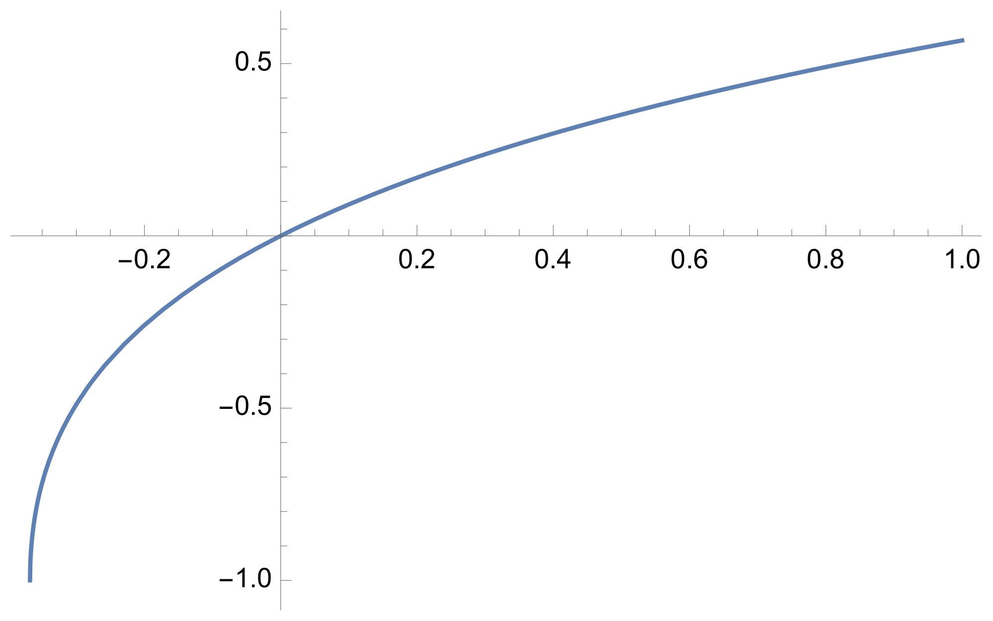
Figure 3.
Principal branch of the function for .

Disclaimer/Publisher’s Note: The statements, opinions and data contained in all publications are solely those of the individual author(s) and contributor(s) and not of MDPI and/or the editor(s). MDPI and/or the editor(s) disclaim responsibility for any injury to people or property resulting from any ideas, methods, instructions or products referred to in the content. |
© 2023 by the authors. Licensee MDPI, Basel, Switzerland. This article is an open access article distributed under the terms and conditions of the Creative Commons Attribution (CC BY) license (https://creativecommons.org/licenses/by/4.0/).
Share and Cite
MDPI and ACS Style
Area, I.; Nieto, J.J. On a Quadratic Nonlinear Fractional Equation. Fractal Fract. 2023, 7, 469. https://doi.org/10.3390/fractalfract7060469
AMA Style
Area I, Nieto JJ. On a Quadratic Nonlinear Fractional Equation. Fractal and Fractional. 2023; 7(6):469. https://doi.org/10.3390/fractalfract7060469
Chicago/Turabian StyleArea, Iván, and Juan J. Nieto. 2023. "On a Quadratic Nonlinear Fractional Equation" Fractal and Fractional 7, no. 6: 469. https://doi.org/10.3390/fractalfract7060469