


Identification of Fractional Models of an Induction Motor with Errors in Variables

1
Department of Information Systems Security, Samara National Research University, 443086 Samara, Russia
2
Department of Mechatronics, Samara State University of Transport, 443066 Samara, Russia
Fractal Fract. 2023, 7(6), 485; https://doi.org/10.3390/fractalfract7060485
Submission received: 25 April 2023
/
Revised: 15 June 2023
/
Accepted: 16 June 2023
/
Published: 18 June 2023
(This article belongs to the Special Issue Application of Fractional Calculus as an Interdisciplinary Modeling Framework, 2nd Edition)
Abstract
:The skin effect in modeling an induction motor can be described by fractional differential equations. The existing methods for identifying the parameters of an induction motor with a rotor skin effect suggest the presence of errors only in the output. The presence of errors in measuring currents and voltages leads to errors in both input and output signals. Applying standard methods, such as the ordinary least squares method, leads to biased estimates in these types of problems. The study proposes a new method for identifying the parameters of an induction motor in the presence of a skin effect. Estimates of parameters were determined based on generalized total least squares. The simulation results obtained showed the high accuracy of the obtained estimates. The results of this research can be applied in the development of predictive diagnostic systems. This study shows that ordinary least squares parameter estimates can lead to incorrect operation of the fault diagnosis system.
1. Introduction
Today, methods for identifying the parameters of induction motors based on equivalent circuits are being actively developed. There are a great number of methods for identifying the parameters of induction motor models. An overview of these identification methods is presented in [1,2].
Estimation of induction motor parameters based on ordinary least squares (OLS) and its recursive modifications is considered in [3,4,5,6]. The application of the total least squares (TLS) technique and its recursive versions was proposed in articles [7,8,9,10,11,12].
The use of integer-order dynamical models leads to significant errors between the measured signals and the results obtained from simulations [13]. The greatest discrepancies are high-power squirrel cage induction machines, in which there is a skin effect in the rotor cage bars and in induction and synchronous machines with a solid rotor [14].
Using high integer-order models that more accurately account for the skin effect in the solid rotor of induction motors leads to a great increase in the number of equivalent circuit elements; however, parameter identification of the high integer-order models is very difficult [15].
Another approach to increase the accuracy of the model is to use the fractional order of the models. Such models cannot be described by traditional electrical circuits. The description of such models requires the use of fractional derivatives.
Fractional-order derivatives are widely used to describe various processes and phenomena. Fractional-order differentiation constitutes a valuable instrument for modeling real-world processes. Fractional calculations are widely used for the synthesis of fractional controllers for various electric motors including, among others, induction motors [16,17,18,19], direct current (DC) motors [20], and permanent magnet synchronous motors (PMSMs) [21]. The aforementioned research on the topic always assumed that induction motor models were of an integer order.
There are far fewer articles devoted to modeling and identification of induction motors by fractional-order models. In [14,22,23,24], the researchers represented the skin effect in a solid rotor by means of resistance and inductance with fixed values and fractional-order inductance, depending on the frequency of induced eddy currents.
The authors of [25] proposed a frequency method for identifying models with fractional-order inductance. Identification of models with fractional-order inductance based on the output error (OE) model was considered in [26].
By monitoring the parameters of an induction motor, faults can be diagnosed. The authors of [27] proposed diagnosing a short circuit in a stator winding by reducing stator resistance and proposed determining broken rotor bars by increasing rotor resistance. Similar diagnostic methods can be applied to fractional-order models. The accuracy of diagnostics depends on the accuracy of the estimated parameters. This makes the development of methods for identifying fractional-order models relevant.
This study is the first to consider the identification of fractional models of induction motors with errors in variables. Previously, either fractional output error models [26] or integer models with errors in variables [7,8,9,10,11] were considered. Currents and voltages are always measured with errors, which leads to the fact that it is necessary to identify a system with noise in the input and output signals. Applying standard methods, such as OLS, lead to biased estimates in these types of problems.
For the first time in one article, three fractional orders of an induction motor model with errors in variables were compared for noise immunity.
It was shown that in the presence of current and voltage measurement errors, generalized total least squares allow one to obtain more accurate parameter estimates than ordinary least squares. This study shows that OLS parameter estimates can lead to incorrect operation of the fault diagnosis system.
2. Materials and Methods
2.1. Problem Statement
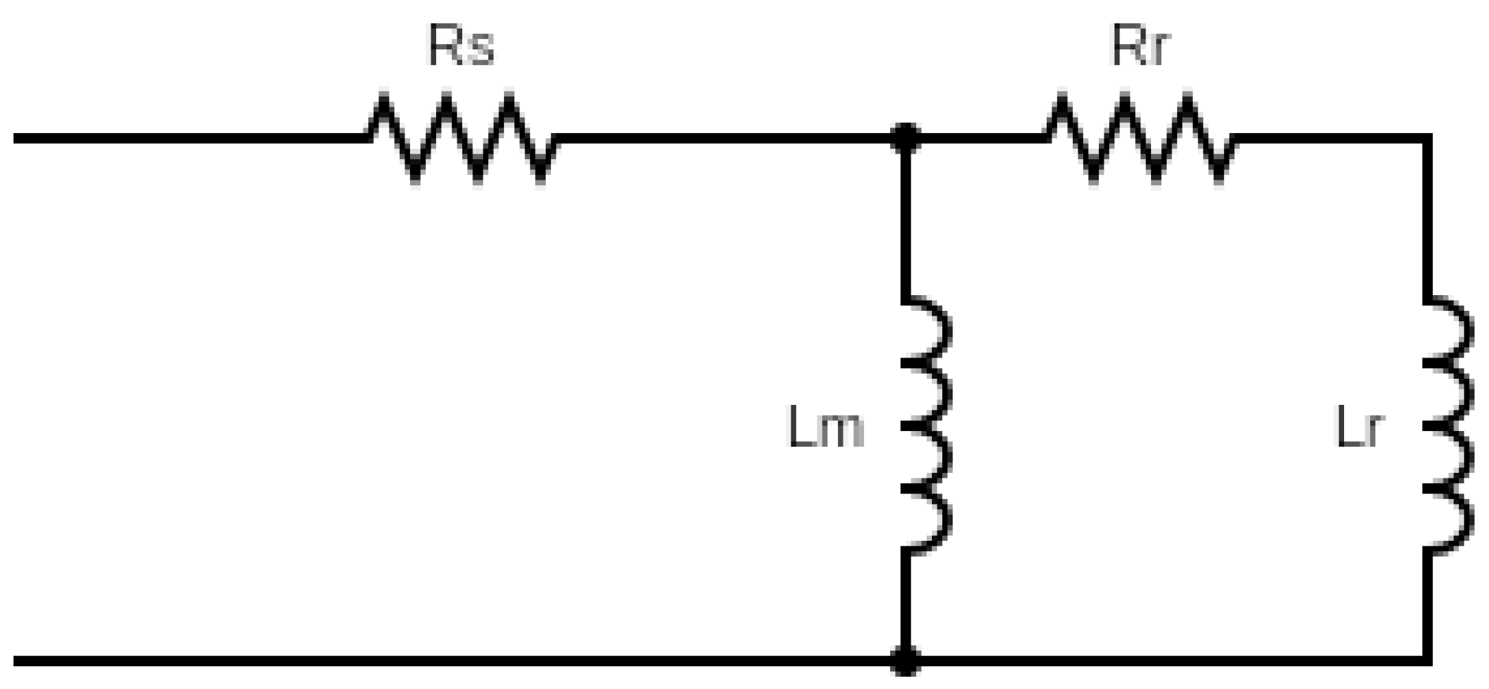
T-form circuit models are more complex than necessary. They can be transformed into simpler models with no loss of information or accuracy [28]. This configuration has been denoted as the Г form, from the structure of its two inductances. Modeling a Γ-equivalent circuit will make a locked rotor for Ω = 0.
The equivalent circuit shown in Figure 1 does not describe the skin effects typical of real induction motors. To simulate skin effects, models with non-integer-order derivatives can be presented. Let us replace the resistor and the inductance with the complex resistance . The equivalent circuit is shown in Figure 2.
The equivalent impedance of an induction motor is defined as:
Various models with derivatives of non-integer order are known. is the one-derivative black box mode [23]:
or the two-derivative model [24]:
Furthermore, there is a three-parameter model [14]:
The relationship between stator current and stator voltage is defined as:
where is the stator voltage and is the stator current.
In real conditions, currents and voltages are always measured with noise:
where and are additive zero-mean white Gaussian noises corrupting the voltage signal and the current signal, and they are assumed not to be correlated with the voltage signal and the current signal.
The problem with identifying an induction motor is the estimation of the vector of unknown parameters from the measured values of the stator current and stator voltage . The parameter vector of impedance (1) for the model (2) is:
For the model (3), the parameter vector of impedance is:
For the model (4), the parameter vector of impedance is:
2.2. GTLS Algorithm for Identification of Induction Motor
Let us express the value of the impedance in terms of the physical parameters of the equivalent circuits. The impedance value (1) for model (2) is:
The impedance value (1) for model (3) is:
The impedance value (1) for model (4) is:
Equation (5) in the time domain for impedances (2)–(4) is defined as:
where is the Grünwald–Letnikov fractional operator, is the sampling period, and is Newton’s binomial generalized to fractional orders.
Equations (13)–(15) in matrix form are described as:
Equation (13) is described as:
, , , , .
Equation (14) is described as:
, , , , ,
Equation (15) is described as:
, , , , .
For noisy current and voltage , Equation (16) is described as:
where
and .
Calculating the fractional derivative from noisy data is a serious problem in identifying a fractional system and leads to large errors. Therefore, the signals must be processed by the state variable filter (SVF) proposed in [29]. The SVF is defined by the following equation:
where the order is an integer chosen such that and denote the filter cut-off frequency. The choice of the number is a compromise between filter complexity and filtering quality. However, increasing the order for large produces a very slight increase in the filtering quality.
The filtered input and output signals and are determined as follows:
Using the filtered input and output signals, Equation (17) can be reformulated as:
Equation (20), in discrete time, is described as:
It is assumed that the fractional order is already known; our goal is to estimate only the fractional differential equation coefficients. We will use generalized total least squares for this. The solving of generalized total least squares is reduced to finding the minimum of the objective function:
where
is the Euclidian norm, is the diagonal matrix of noise variances, and where .
Total least squares regression assumes that the noise variance is the same in all columns and in the right side. This assumption is not satisfied for Equation (22). Calculating the exact value of the noise variances of each column is a very difficult task. We will assume that the use of the SVF filter makes it possible to achieve an approximately equal signal-to-noise ratio in each column. Then, normalization will make it possible to obtain approximately equal noise variances in each column. The standard deviations for each column can be defined as:
where is j-th column of the matrix .
The generalized total least squares problem (22) can be reduced to the total least squares problem [30]:
where .
The minimum of function (24) can be found as a solution to the biased normal system of equations [31]:
where is the minimal singular values of matrices and is the identity matrix.
An augmented symmetric system of equations used to solve total least squares (16) [32] can be expressed as follows:
An inverse change of variable can be performed as follows: .
Let us determine the parameter estimates from the estimates . For impedance model (2), this would be carried out as follows:
For impedance model (3), this would be carried out as follows:
For impedance model (4), this would be carried out as follows:
If the order of differentiation is unknown, as is often the case in practice, order estimation must be considered along with transfer function coefficient estimation. The use of generalized total least squares is possible when the fractional order is known a priori. This section describes an algorithm for extending the identification method presented above for the case when the order of differentiation is unknown. The algorithm is based on a combination of a generalized least squares method for estimating coefficients and a nonlinear algorithm for optimizing the order of differentiation. The parameter identification problem is presented as a functional minimization. Therefore, the main goal of this approach is to reduce the residual error with respect to .
The objective function (31) depends on one parameter. From a priori knowledge, it follows that for the impedance model (2) and for models (2) and (3). The minimum of a function can be found by one of the standard methods for optimizing a function of one variable.
3. Simulation Results
MATLAB was used for simulation. Test cases were compared to the normalized root-mean-square error (NRMSE) of parameter estimation, defined as:
The parameter estimates obtained on the basis of GTLS from objective functions (22) and (31) were compared with LS estimates defined as:
The FOMCON toolbox [33] was used to model the fractional order of the transfer functions. The sample period was set at h = 0.0002 s. The number of data points N in each simulation was 10,000.
Example 1.
The impedance model is described by Equation (2). The true parameter vector is:
The conductivity function is defined as:
The ratio of standard deviations “signal-noise ratio” is
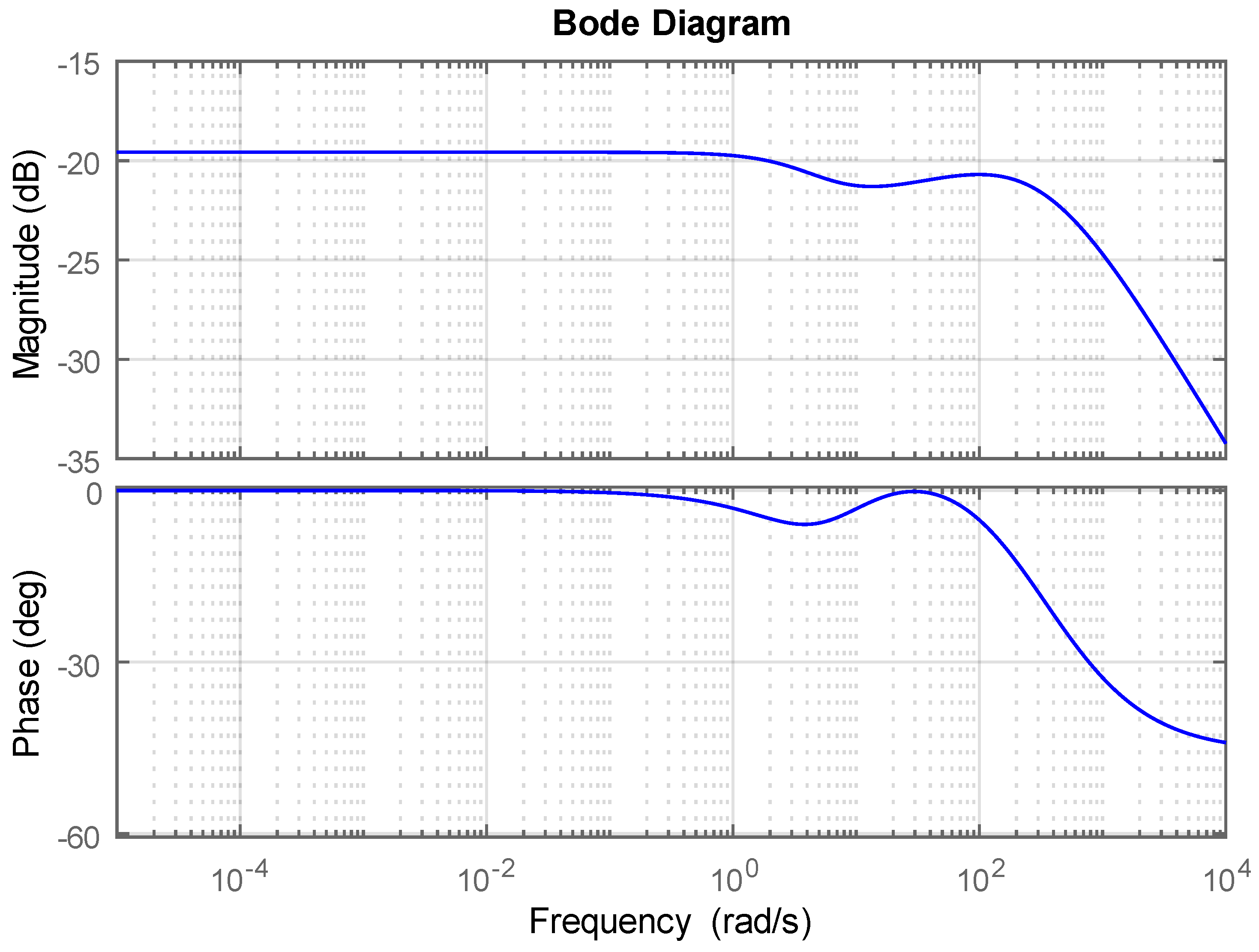
Figure 3 shows the Bode diagram of the system defined by (37).
Selection of the SVF filters are chosen as:
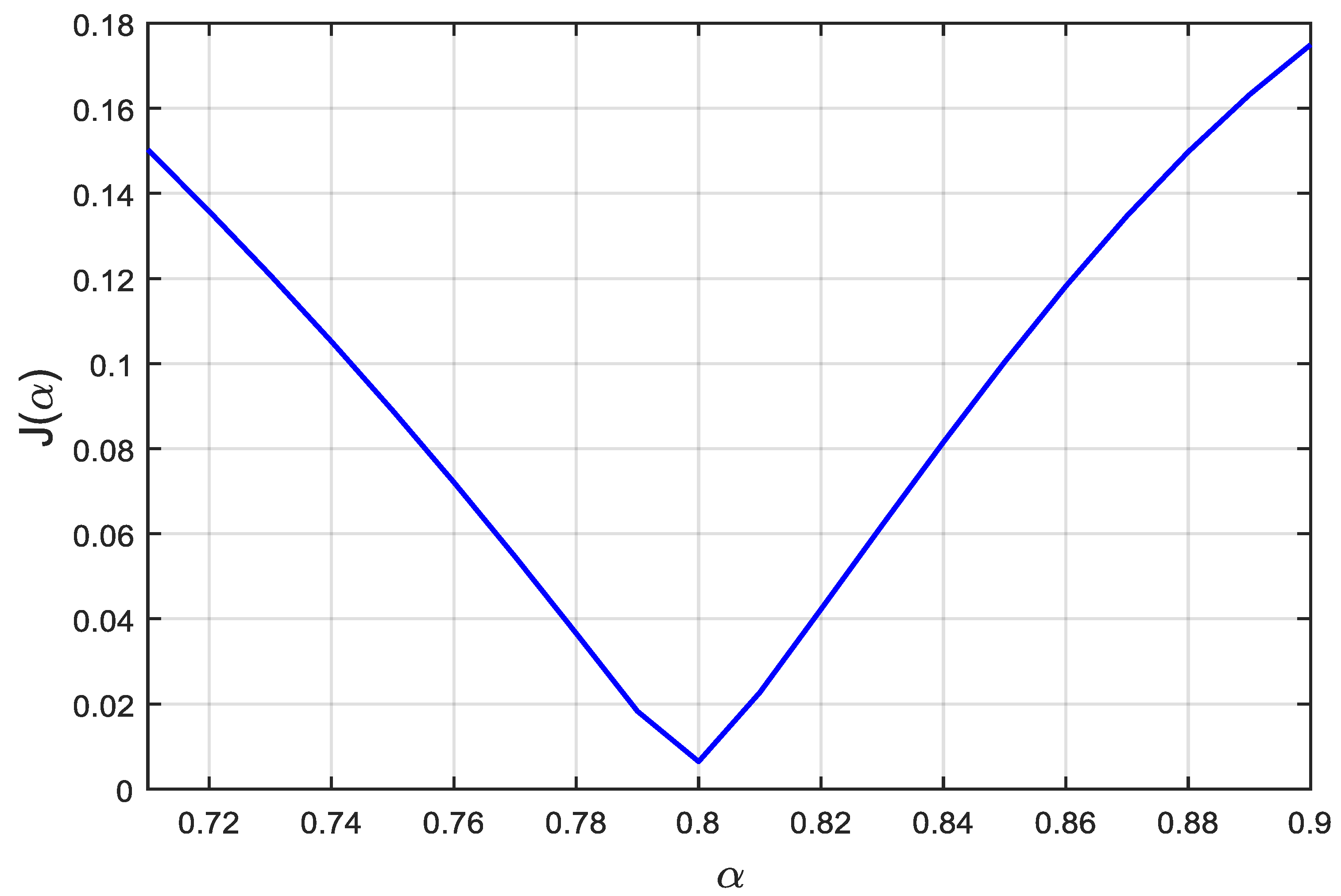
Figure 4 shows the objective function (35) of the system (37).
Figure 5 shows the objective function (31) of the system (37).
Table 1 shows parameter estimates and NRMSE (SNR = 100).
Table 2 shows parameter estimates and NRMSE (SNR = 100).
Example 2.
The impedance model is described by Equation (3). The true parameter vector is
The conductivity function is defined as
The ratio of standard deviations “signal-noise ratio” is
Figure 6 shows the Bode diagram of the system defined by (40).
Selection of the SVF filters are chosen as:
Table 3 shows parameter estimates and NRMSE (SNR = ).
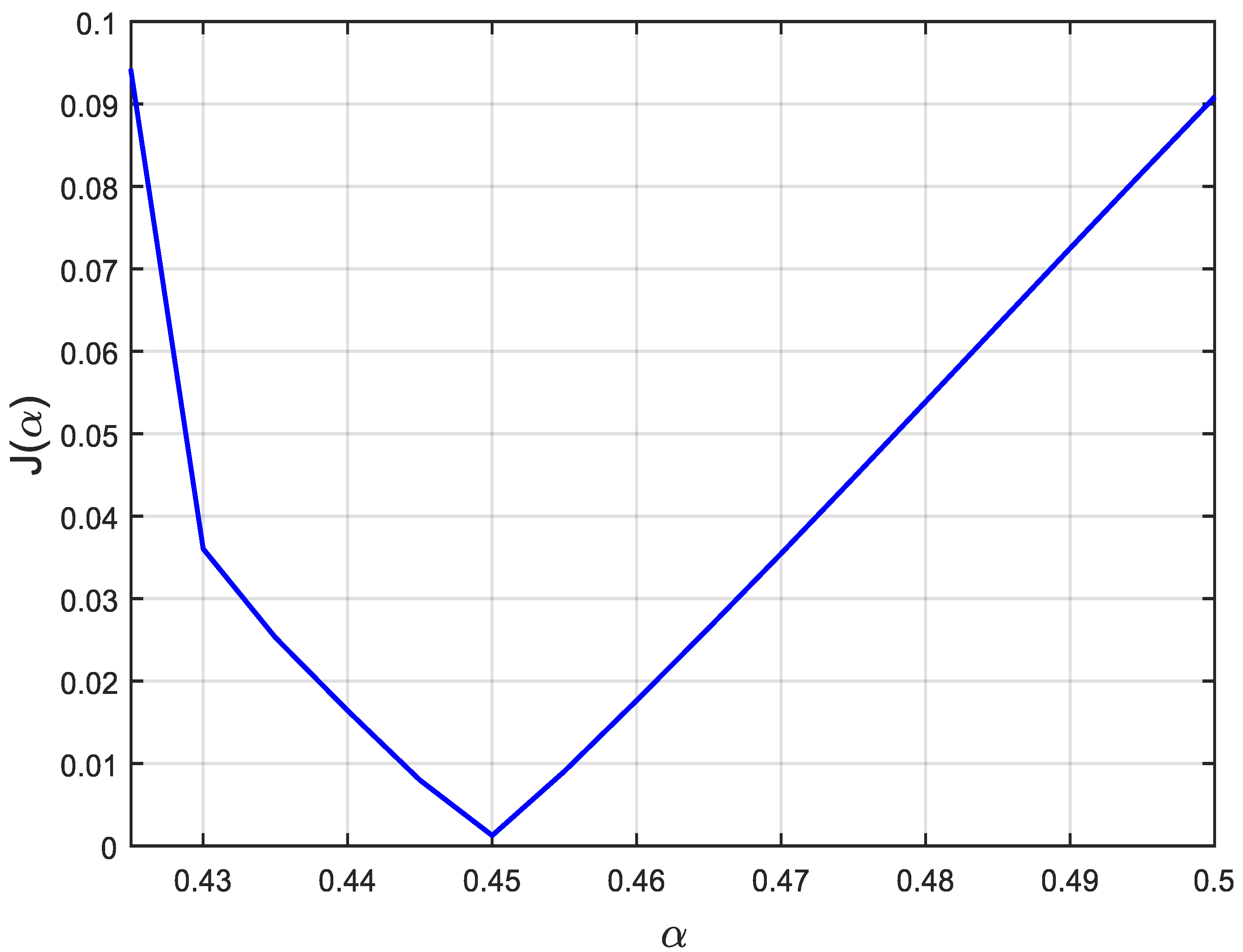
Figure 7 shows the objective function (35) of the system (40).
Figure 8 shows the objective function (31) of the system (40).
Table 4 shows parameter estimates and NRMSE (SNR = ).
Example 3.
The impedance model is described by Equation (3). The true parameter vector is
The conductivity function is defined as
The ratio of standard deviations “signal-noise ratio” is
Figure 9 shows the Bode diagram of the system defined by (43).
Selection of the SVF filters are chosen as:
Figure 10 shows the objective function (35) of the system (43).
Figure 11 shows the objective function (31) of the system (43).
Table 5 shows parameter estimates and NRMSE (SNR = 1000).
Table 6 shows parameter estimates and NRMSE (SNR = 1000).
The results shown in Examples 1–3 show that the ordinary least squares method has more inaccurate estimates than the proposed modification of GTLS. Examples 1 and 3 illustrate how the presence of noise affects the appearance of a false fault. In example 1, the true resistance of the rotor and its estimates are , and . In example 3, the resistance of the rotor and its estimates are , and . The OLS ratings are highly inflated, which can be misinterpreted as broken rotor bars.
4. Discussion
The simulation results show that model (1) allows the identification of parameters at the lowest signal-to-noise ratio. The disadvantage of this model is poor accuracy at high frequencies. Model (2) is the most accurate of those considered in this study. However, it is very sensitive to noise. It should be noted that due to the presence of the first-order derivative and the derivative of the order in the regression vector, the problem is ill-conditioned. Model (3) occupies an intermediate position between model (1) and model (2); it is less resistant to noise than (1), but it has an accuracy comparable to (2). For construction, the experimental model (3) is the most preferable.
5. Conclusions
This article is the first to consider the identification of three fractional-order models of an induction motor in the presence of errors in variables. Fractional-order models allow one to simulate the skin effect. Further development of identification methods can include the construction of algorithms based on regularized total least squares [34,35] and the use of implicit models of transfer functions [36,37].
Funding
The work was carried out as part of the implementation of the program for the development of the Scientific and Educational Mathematical Center of the Volga Federal District, Agreement No. 075-02-2023-931.
Data Availability Statement
The data was generated in Matlab. Simulation conditions are described in detail in the corresponding section.
Acknowledgments
The author is grateful to the reviewers for their constructive and useful comments, which made it possible to significantly improve the presentation of the results obtained.
Conflicts of Interest
The author declares no conflict of interest.
References
- Toliyat, H.A.; Levi, E.; Raina, M. A review of RFO induction motor parameter estimation techniques. IEEE Trans. Energy Convers. 2003, 18, 271–283. [Google Scholar] [CrossRef]
- Zhan, X.; Zeng, G.; Liu, J.; Wang, O.; Ou, S. A Review on Parameters Identification Methods for Asynchronous Motor. Int. J. Adv. Comput. Sci. Appl. 2015, 6, 104–109. [Google Scholar] [CrossRef] [Green Version]
- Tang, J.; Yang, Y.; Blaabjerg, F.; Chen, J.; Diao, L.; Liu, Z. Parameter Identification of Inverter-Fed Induction Motors: A Review. Energies 2018, 11, 2194. [Google Scholar] [CrossRef] [Green Version]
- Stephan, J.; Bodson, M.; Chiasson, J. Real-time estimation of the parameters and fluxes of induction motors. IEEE Trans. Ind. Electron. 1994, 30, 746–759. [Google Scholar] [CrossRef]
- Cirrincione, M.; Pucci, M. Experimental verification of a technique for the real-time identification of induction motors based on the recursive least-squares. In Proceedings of the International Workshop on Advanced Motion Control. Proceedings (Cat. No. 02TH8623), Maribor, Slovenia, 3–5 July 2002; pp. 326–334. [Google Scholar]
- Alonge, F.; D’Ippolito, F.; Barbera, S.L.; Raimondi, F.M. Parameter identification of a mathematical model of induction motors via least squares techniques. In Proceedings of the 1998 IEEE International Conference on Control Applications (Cat. No. 98CH36104), Trieste, Italy, 1–4 September 1998; pp. 491–496. [Google Scholar]
- Cirrincione, M.; Pucci, M.; Vitale, G. Power Converters and AC Electrical Drives with Linear Neural Networks; CRC Press: Boca Raton, FL, USA; Taylor & Francis Group: Abingdon, UK , 2012. [Google Scholar]
- Moons, C.; De Moor, B. Parameter identification of induction motor drives. Automatica 1995, 31, 1137–1147. [Google Scholar] [CrossRef]
- Cirrincione, M.; Cirrincione, G.; Pucci, M.; Jaafari, A. The estimation of the induction motor parameters by the GeTLS EXIN neuron. In 2010 IEEE Energy Conversion Congress and Exposition; IEEE: Piscataway, NJ, USA, 2010; pp. 1680–1685. [Google Scholar]
- Cirrincione, G.; Cirrincione, M. Neural Based Orthogonal Data Fitting: The EXIN Neural Networks Series: Adaptive and Learning Systems for Signal Processing, Communications and Control; Wiley & Sons: New York, NY, USA, 2010. [Google Scholar]
- Ivanov, D.V.; Sandler, E.A.; Chertykovtseva, N.V.; Tikhomirov, E.A.; Semenova, N.S. Identification of induction motor parameters with measurement errors. IOP Conf. Ser. Mater. Sci. Eng. 2019, 560, 012163. [Google Scholar] [CrossRef]
- Ivanov, D.V.; Sandler, I.L.; Chertykovtseva, N.V. Generalized total least squares for identification of electromagnetic parameters of an induction motor. IOP J. Phys. Conf. Ser. 2021, 2032, 012093. [Google Scholar] [CrossRef]
- Canay, I. Causes of Discrepancies on Calculation of Rotor Quantities and Exact Equivalent Diagrams of the Synchronous Machines. IEEE Trans. Power Appar. Syst. 1969; PAS-88, 1114–1645. [Google Scholar]
- Staszak, J. Solid-Rotor Induction Motor Modeling Based on Circuit Model Utilizing Fractional-Order Derivatives. Energies 2022, 15, 6371. [Google Scholar] [CrossRef]
- Kabbaj, H.; Roboam, X.; Lefevre, Y.; Faucher, J. Skin effect characterization in a squirrel cage induction machine. In Proceedings of the ISIE’97 Proceeding of the IEEE International Symposium on Industrial Electronics, Guimaraes, Portugal, 7–11 July 1997; Volume 2, pp. 532–536. [Google Scholar] [CrossRef]
- Saleem, A.; Soliman, H.; Al-Ratrout, S.; Mesbah, M. Design of a fractional order PID controller with application to an induction motor drive. Turk. J. Electr. Eng. Comput. Sci. 2018, 26, 2768–2778. [Google Scholar] [CrossRef]
- Adigintla, S.; Aware, M.V. Position Control of the Induction Motor using Fractional Order Controllers. In Proceedings of the 2020 International Conference on Power, Instrumentation, Control and Computing (PICC), Thrissur, India, 17–19 December 2020; pp. 1–6. [Google Scholar] [CrossRef]
- Yu, Y.; Liu, X. Model-Free Fractional-Order Sliding Mode Control of Electric Drive System Based on Nonlinear Disturbance Observer. Fractal Fract. 2022, 6, 603. [Google Scholar] [CrossRef]
- Nosheen, T.; Ali, A.; Chaudhry, M.U.; Nazarenko, D.; Shaikh, I.u.H.; Bolshev, V.; Iqbal, M.M.; Khalid, S.; Panchenko, V. A Fractional Order Controller for Sensorless Speed Control of an Induction Motor. Energies 2023, 16, 1901. [Google Scholar] [CrossRef]
- John, D.A.; Sehgal, S.; Biswas, K. Hardware Implementation and Performance Study of Analog PIλDμ Controllers on DC Motor. Fractal Fract. 2020, 4, 34. [Google Scholar] [CrossRef]
- Zheng, W.; Huang, R.; Luo, Y.; Chen, Y.; Wang, X.; Chen, Y. A Look-Up Table Based Fractional Order Composite Controller Synthesis Method for the PMSM Speed Servo System. Fractal Fract. 2022, 6, 47. [Google Scholar] [CrossRef]
- Kabbaj, H. Identification d’un Modèle Type Circuit Prenant en Compte les Effets de Fréquences dans une Machine Asynchrone à Cage D’écureuil. Ph.D. Thesis, INPT, Toulouse, France, 1997. [Google Scholar]
- Trigeassou, J.C.; Poinot, T.; Lin, J.; Oustaloup, A.; Levron, F. Modelling and identification of a non integer order system. In Proceedings of the 1999 European Control Conference (ECC), Karlsruhe, Germany, 31 August–3 September 1999. [Google Scholar]
- Benchellal, A.; Poinot, T.; Trigeassou, J.C. Approximation and identification of diffusive interfaces by fractional models. Signal Process. 2006, 86, 2712–2727. [Google Scholar] [CrossRef]
- Canat, S.; Faucher, J. Modelling and simulation of induction machine with fractional derivative. In Proceedings of the IProc FDA’04, Bordeaux, France, 19–20 July 2004; pp. 393–399. [Google Scholar]
- Jalloul, A.; Trigeassou, J.K.; Jelassi, K.; Melchior, P. Fractional Order of Rotor Skin Effect in Induction Machines. Nonlinear Dyn. 2013, 73, 801–813. [Google Scholar] [CrossRef]
- Bachir, S.; Tnani, S.; Trigeassou, J.-C.; Champenois, G. Diagnosis by parameter estimation of stator and rotor faults occurring in induction machines. IEEE Trans. Ind. Electron. 2006, 53, 963–973. [Google Scholar] [CrossRef]
- Slemon, G.R. Modelling of induction machines for electric drives. IEEE Trans. Ind. Appl. 1989, 25, 1126–1131. [Google Scholar] [CrossRef]
- Victor, S.; Malti, R.; Garnier, H.; Oustaloup, A. Parameter and differentiation order estimation in fractional models. Automatica 2013, 49, 926–935. [Google Scholar] [CrossRef]
- Van Huffel, S.; Vandewalle, J. Analysis and properties of the generalized total least squares problem AX ≈ B when some or all columns in A are subject to error. SIAM J. Matrix Anal. Appl. 1989, 10, 294–315. [Google Scholar] [CrossRef]
- Zhdanov, A.I. The solution of ill-posed stochastic linear algebraic equations by the maximum likelihood regularization method. USSR Comput. Math. Math. Phys. 1988, 28, 93–96. [Google Scholar] [CrossRef]
- Ivanov, D.; Zhdanov, A. Symmetrical Augmented System of Equations for the Parameter Identification of Discrete Fractional Systems by Generalized Total Least Squares. Mathematics 2021, 9, 3250. [Google Scholar] [CrossRef]
- Tepljakov, A. FOMCON: Fractional-Order Modeling and Control Toolbox. In Fractional-Order Modeling and Control of Dynamic Systems; Springer: Cham, Switzerland, 2017. [Google Scholar] [CrossRef]
- Golub, G.H.; Hansen, P.C.; O’Leary, D.P. Tikhonov regularization and total least squares. SIAM J. Matrix Anal. Appl. 1999, 21, 185–194. [Google Scholar] [CrossRef] [Green Version]
- Ivanov, D.; Zhdanov, A. Implicit iterative algorithm for solving regularized total least squares problems. Vestn. Samar. Gos. Tekhnicheskogo Univ. Seriya Fiz.-Mat. Nauk. 2022, 26, 311–321. [Google Scholar] [CrossRef]
- Riu, D.; Retière, N.; Ivanès, M. Diffusion phenomenon modelling by half-order systems: Application to squirrel-cage induction machine. J. Magn. Magn. Mater. 2002, 242–245, 1243–1245. [Google Scholar] [CrossRef]
- Machado, T.; Galhano, J.A. Fractional order inductive phenomena based on the skin effect. Nonlinear Dyn. 2012, 68, 107–115. [Google Scholar] [CrossRef]
Figure 1.
Γ-equivalent circuit model of an induction motor.

Figure 2.
Γ-equivalent circuit model of an induction motor with fractional impedance.

Figure 3.
The bode diagrams of the system (37).

Figure 4.
function of the system (37).

Figure 5.
function of the system (37).

Figure 6.
The bode diagrams of the system (40).

Figure 7.
function of the system (40).

Figure 8.
function of the system (40).

Figure 9.
The bode diagrams of the system (43).

Figure 10.
function of the system (43).

Figure 11.
function of the system (43).


Table 1.
The parameter estimates and NRMSE (SNR = 100).
| 7.7348 | 1.5701 | |||
| 0.2140 | 0.2111 | 1.3780 | 0.2207 | 3.1084 |
| 0,0175 | 0.0183 | 4.4481 | 98.9797 | |
| 0.0166 | 0.0162 | 2.5177 | 0.173 | 3.8664 |
| 0.0018 | 0.0021 | 16.6910 | 83.5653 | |
| 0.1050 | 0.1047 | 0.3104 | 0.1047 | 0.3398 |
Table 2.
The parameter estimates and NRMSE (SNR = 100).
| 9.52 | 9.5496 | 0.3114 | 9.5525 | 0.3409 | |
| 0.53 | 0.5368 | 1.2863 | 0.5316 | 0.2928 | |
| 57.03 | 62.4117 | 9.4336 | 56.1215 | 1.5930 | |
| 17.04 | 5.6653 | 28.4394 | 17.4248 | 2.2584 | |
| 0.8 | 0.8134 | 1.6750 | 0.8012 | 0.150 |
Table 3.
The parameter estimates and NRMSE (SNR = ).
| 3.1195 | 0.0708 | |||
| 0.0100 | 0.4765 | 0.0100 | 0.0238 | |
| 0.0175 | 0.0151 | 13.8781 | 0.0164 | 6.4449 |
| 0.2140 | 0.2151 | 0.5211 | 0.2151 | 0.4967 |
| 0.1597 | 0.1590 | 0.4185 | 0.1601 | 0.2315 |
| 2.7572 | 0.7486 | |||
| 898.76 | 68.453 | |||
| 0.0166 | 0.0176 | 5.6452 | 0.0167 | 0.4351 |
| 0.0168 | 0.0167 | 0.2109 | 0.0168 | 0.02053 |
| 0.1050 | 0.1051 | 0.1050 |
Table 4.
The parameter estimates and NRMSE (SNR = ).
| 9.52 | 9.5206 | 0.0065 | 9.5199 | 0.0049 | |
| 0.53 | 0.5280 | 0.3726 | 0.5301 | 0.0269 | |
| 57.04 | 58.6432 | 2.8287 | 57.0057 | 0.0427 | |
| 9.11 | 9.3285 | 2.3998 | 9.1272 | 0.1888 | |
| 17.04 | 18.5816 | 9.0469 | 17.1035 | 0.3724 | |
| 0.12 | 0.1264 | 5.3507 | 0.1172 | 2.3531 | |
| 0.45 | 0.445 | 1.1111 | 0.449 | 0.2222 |
Table 5.
The parameter estimates and NRMSE (SNR = 1000).
| 200.02 | 1.9783 | |||
| 0.0853 | 0.0890 | 4.2894 | 0.0851 | 0.2677 |
| 0.6806 | 0.710 | 4.3891 | 0.6810 | 0.0539 |
| 1.5329 | 1.7989 | 17.3489 | 1.5425 | 0.6201 |
| 0.0656 | 0.0669 | 1.9870 | 0.0655 | 0.1878 |
| 0.1610 | 0.1904 | 18.2696 | 0.1622 | 0.7486 |
| 0.1050 | 0.1044 | 0.5747 | 0.1049 | 0.1136 |
Table 6.
The parameter estimates and NRMSE (SNR = 1000).
| 9.52 | 9.5206 | 0.3584 | 9.5308 | 0.1137 | |
| 0.53 | 0.4281 | 19.2259 | 0.5247 | 1.0108 | |
| 0.85 | 1.2154 | 42.3944 | 0.8506 | 0.0744 | |
| 0.0012 | 0.0015 | 28.4394 | 0.0012 | 0.9381 | |
| 1.3030 | 1.5407 | 18.2424 | 1.3152 | 1.7956 | |
| 0.45 | 0.442 | 1.1778 | 0.451 | 0.222 |
Disclaimer/Publisher’s Note: The statements, opinions and data contained in all publications are solely those of the individual author(s) and contributor(s) and not of MDPI and/or the editor(s). MDPI and/or the editor(s) disclaim responsibility for any injury to people or property resulting from any ideas, methods, instructions or products referred to in the content. |
© 2023 by the author. Licensee MDPI, Basel, Switzerland. This article is an open access article distributed under the terms and conditions of the Creative Commons Attribution (CC BY) license (https://creativecommons.org/licenses/by/4.0/).
Share and Cite
MDPI and ACS Style
Ivanov, D. Identification of Fractional Models of an Induction Motor with Errors in Variables. Fractal Fract. 2023, 7, 485. https://doi.org/10.3390/fractalfract7060485
AMA Style
Ivanov D. Identification of Fractional Models of an Induction Motor with Errors in Variables. Fractal and Fractional. 2023; 7(6):485. https://doi.org/10.3390/fractalfract7060485
Chicago/Turabian StyleIvanov, Dmitriy. 2023. "Identification of Fractional Models of an Induction Motor with Errors in Variables" Fractal and Fractional 7, no. 6: 485. https://doi.org/10.3390/fractalfract7060485