Hybrid Impulsive Feedback Control for Drive–Response Synchronization of Fractional-Order Multi-Link Memristive Neural Networks with Multi-Delays

Abstract

This article addresses the issue of drive–response synchronization in fractional-order multi-link memristive neural networks (FMMNN) with multiple delays, under hybrid impulsive feedback control. To address the impact of multiple delays on system synchronization, an extended fractional-order delayed comparison principle incorporating impulses is established. By leveraging Laplace transform, Mittag–Leffler functions, the generalized comparison principle, and hybrid impulsive feedback control schemes, several new sufficient conditions are derived to ensure synchronization in the addressed FMMNN. Unlike existing studies on fractional-order single-link memristor-based systems, our response network is a multi-link model that considers impulsive effects. Notably, the impulsive gains ${\alpha }_i$ are not limited to a small interval, thus expanding the application range of our approach (${\alpha }_i\in (-2,0)\cup (-\infty ,-2)\cup (0,+\infty )$). This feature allows one to choose impulsive gains and corresponding impulsive intervals that are appropriate for the system environment and control requirements. The theoretical results obtained in this study contribute to expanding the relevant theoretical achievements of fractional-order neural networks incorporating memristive characteristics.

1. Introduction

Memristive neural networks (MNNs) are a class of state-dependent switching models that have been widely applied in various fields, including machine learning, stability analysis, image encryption, and fault detection [1,2,3,4,5,6]. Due to the memory characteristics of memristors, which are similar to the behavior of neuronal synapses, MNNs can model the working mechanisms of neurons in the human brain effectively. Moreover, memristor-based neural networks significantly improve the parallel computing and adaptive capabilities of conventional network models. Many researchers have investigated the dynamic behavior of neural networks, with synchronization being one of the most significant aggregation behaviors, which naturally attracts a lot of attention [7,8].

Currently, there exist several notable research contributions related to the synchronization of MNN. For example, Bao et al. [9] investigated the exponential synchronization of MNN with stochastic features and various delays under the Filippov framework. Li et al. [10] focused on the drive–response synchronization of MNN with delayed coupling and discrete activation functions in finite time. Yu et al. [11] discussed the finite-time synchronization of memristor-based neural networks with complex variable parameters using the Lyapunov stability theory. In [12], Yang et al. studied the global synchronization of nonlinear coupled neural networks, including uncertain disturbances, and obtained sufficient conditions by employing hybrid control schemes and graph topologies. The finite-time synchronization problems of uncertain MNN were addressed in [13], and more practical synchronization criteria were derived via aperiodically intermittent adjustment. Furthermore, various other research results on memristive neural networks can be found in [14,15,16].

Most research on network synchronization has mainly focused on integer-order neural networks. However, fractional calculus, which is a significant theoretical extension of integer calculus, provides a regulable free degree to classical calculus and has several distinct properties, including infinite memory and heredity, that the integer calculus operator does not possess [17,18]. Furthermore, the key advantage of the extension operator is the nonlocality, which means its future state is not only related to the current state information but also related to the past state information [19,20,21]. As a result, fractional-order systems can more accurately describe natural phenomena, especially actual change processes, such as Fourier heat conduction, viscoelastic phenomena, and reaction–diffusion processes. However, increasing the degree of freedom improves the simulation accuracy but also makes the fractional-order model exhibit more complex properties [22,23,24]. Due to the particularity of fractional calculus operators, the stability theory of traditional integer-order systems is not applicable to fractional-order models.

Recently, there has been growing interest in the synchronization of fractional-order memristive neural networks (FMNN). For instance, Chen et al. [25] explored the global synchronization problem of FMNN without delays using a continuous state feedback control method. Bao et al. [26] investigated the global projective synchronization for a class of FMNNs via adaptive feedback control technologies. In [27], Jiang et al. considered drive–response synchronization of generalized FMNN in finite time under a memoryless controller. However, these studies did not consider the effect of time delays on system stability. Time delays are inevitable in the process of neuronal information transmission in memristor-based neural networks due to limited transmission speed and communication congestion. To obtain a more realistic synchronization criterion, a constant time delay was introduced into the fractional-order memristive model in [28]. Subsequently, more fractional-order memristive systems involving time delays have attracted researchers’ attention. For example, Velmurugan et al. [29] proposed a method to achieve global projective synchronization of FMNN including time delays based on differential inclusion and fractional-order stability theories as well as linear feedback control. The drive–response synchronization of delayed FMNN with an order $\mu \in (0,1)$ or $\mu \in (1,2)$ in finite time was studied in [30], while the global synchronization of FMNN containing multi-delays was deliberated by building a generalized fractional-order delayed comparison principle without impulses in [31]. Several other interesting results about the synchronization of FMNN can be found in [32,33].

Notably, most existing studies have focused on the synchronization of single-link systems based on continuous feedback control methods, while few works have addressed the drive–response synchronization of FMMNN with multi-delays using hybrid impulsive feedback control schemes. In memristive neural networks, multi-link structures refer to the presence of multiple connections or links between the neurons in the network. Compared with single-link structures, the multi-link structure allows for the formation of more complex and intricate neural pathways, which can enable the network to perform more complex computations and facilitate the emergence of collective behavior, enhance the robustness and fault tolerance of the network by providing redundant pathways for signal transmission, and improve the learning ability of the network by allowing for the reinforcement of specific pathways and the suppression of others. Therefore, when studying memristive neural networks, it is important to consider the impact of multi-link structures on the network’s behavior and performance.

However, it is evident that conventional impulsive control techniques and delayed comparison principles are insufficient to address the synchronization problems in fractional-order neural networks, particularly in the case of multi-delay neural networks with multiple links utilizing impulsive control. Achieving synchronization in such networks remains a challenging and unresolved issue. Therefore, this study aims to establish a fractional-order multi-delay comparison principle that incorporates impulses to overcome this challenge and investigate the drive–response synchronization of FMMNN with multi-delays. The key contributions of this research are as follows. Firstly, unlike prior studies [25,26,27,28,29,30] concerning fractional-order single-link memristor-based systems, our drive and response networks contain multi-links, and multi-delays and impulsive are also included in our model. Secondly, the effects of impulses were neglected in the existing fractional-order comparison principles in [19,23,31], while we construct a more generalized fractional-order comparison principle that incorporates multi-delays and impulses to address the impact of delays on system stability. Thirdly, hybrid impulsive feedback control schemes are proposed to achieve synchronization in FMMNN, with the advantages of simple implementation and increased safety during signal transmission, which improves pure state feedback control schemes utilized in previous studies [31,32,33]. It should be also mentioned that the impulsive gain in [7] is limited to the interval $(-2,0)$. Notably, in this paper, the impulsive gains in the proposed synchronization conditions can be selected to be any value except $-2$ and 0, which are not limited to a small interval as in the previous literature. Finally, several novel synchronization criteria dependent on the impulsive interval, fractional order, and control gains are derived to ensure the drive–response synchronization of FMMNN.

2. Preliminary Knowledge and Mathematical Model

In this section, we begin by providing an overview of some important definitions, assumptions, and lemmas. We then introduce an extended fractional-order multi-delay comparison principle that incorporates impulses and present a mathematical model.

Definition 1.

The fractional integral for an integrable function $\mathfrak{C}\left(t\right)$ is defined as

$$\begin{array}{c}\hfill I_t^{\mu }\mathfrak{C}\left(t\right)=\frac{1}{\mathsf{\Gamma }\left(\mu \right)}{\int }_{t_0}^t{(t-\overline{\tau })}^{\mu -1}\mathfrak{C}\left(\overline{\tau }\right)d\overline{\tau },\end{array}$$

where $t\ge t_0$, $\mathsf{\Gamma }\left(\mu \right)={\int }_0^{\infty }{t}^{\mu -1}{e}^{-t}dt$, and $\mu >0$ represents the order [18].

Definition 2.

The Liouville–Caputo fractional derivative for a differentiable function $\mathfrak{C}\left(t\right)$ is defined as

$$\begin{array}{c}\hfill {}^{LC}{D}_t^{\mu }\mathfrak{C}\left(t\right)=\frac{1}{\mathsf{\Gamma }(m-\mu )}{\int }_{t_0}^t{(t-\overline{\tau })}^{m-\mu -1}{\mathfrak{C}}^{\left(m\right)}\left(\overline{\tau }\right)d\overline{\tau },\end{array}$$

where $t\ge t_0$, $0\le m-1<\mu <m$, and $m\in Z_{+}$ [18].

Definition 3.

The Mittag–Leffler function containing one parameter is defined by

$$\begin{array}{c}\hfill E_{\mu }\left(z\right)={\displaystyle \sum _{k=0}^{\infty }}\frac{z^k}{\mathsf{\Gamma }(\mu k+1)},\end{array}$$

where $\mu >0$, and $z\in C$ [18].

Remark 1.

The Liouville–Caputo derivative is used to establish fractional-order neural network models in this study since the starting conditions of fractional differential systems including the Liouville–Caputo derivative have similar modalities as integer-order differential systems, which have acceptable physical meanings.

Assumption 1.

The feedback functions ${\beta }_j$, ${\gamma }_j$, ${\beta }_j(\pm T_j)={\gamma }_j(\pm T_j)=0$, conform to the following Lipschitz conditions

$$\begin{array}{c}\hfill |{\beta }_j\left(v\right)-{\beta }_j\left(w\right)|\le {\tilde{\beta }}_j|v-w|,|{\gamma }_j\left(v\right)-{\gamma }_j\left(w\right)|\le {\tilde{\gamma }}_j|v-w|,({\tilde{\beta }}_j>0,{\tilde{\gamma }}_j>0),\end{array}$$

for $\forall v,w\in R$, and $j=1,2,\cdots ,n$.

Assumption 2.

For the bounded feedback functions ${\beta }_j$ and ${\gamma }_j$, there exist constants $M_j\in R$, ${\overline{M}}_j\in R$, such that

$$\begin{array}{c}\hfill |{\beta }_j\left(v\right)|\le M_j,\left|{\gamma }_j\left(v\right)\right|\le {\overline{M}}_j,\end{array}$$

hold for $\forall v\in R$, $j=1,2,\cdots ,n$.

Consider a class of fractional-order multi-link memristive neural networks including multi-delays, which can be characterized by

$${}^{LC}{D}_t^{\mu }{v}_i\left(t\right)=-b_i{v}_i\left(t\right)+{\displaystyle \sum _{j=1}^n}{c}_{ij}\left(v_i\left(t\right)\right){\beta }_j\left(v_j\left(t\right)\right)+{\displaystyle \sum _{m=1}^h}{\displaystyle \sum _{j=1}^n}{d}_{ij}^m\left(v_i\left(t\right)\right){\gamma }_j\left(v_j(t-{\tau }_m)\right)+I_i,t\ge 0,$$

(1)

where $i=1,2,\cdots ,n,$ and $0<\mu <1$. $b_i>0$ represents the self-feedback connection parameter. ${\tau }_m$ is the mth transmission delay and $I_i$ is the external input. $v_j\left(t\right)$ represents the state variable affiliated with the jth neuron. ${\beta }_j\left(v_j\left(t\right)\right)$ and ${\gamma }_j\left(v_j(t-{\tau }_m)\right)$ denote the non-delay and delayed feedback functions. The initial values of neural networks (1) are $v\left(s\right)=\chi \left(s\right)={({\chi }_1\left(s\right),{\chi }_2\left(s\right),\cdots ,{\chi }_n\left(s\right))}^T\in \mathcal{C}([-\tau ,0],R^n)$, where $\tau =max\{{\tau }_1,{\tau }_2,\cdots ,{\tau }_h\}$. Based on the peculiarities of the memristor and current voltage, $c_{ij}\left(v_i\left(t\right)\right)$ and $d_{ij}^m\left(v_i\left(t\right)\right)$ stand for memristive connective weights meeting the requirements below:

$$\begin{array}{c}\hfill c_{ij}\left(v_i\left(t\right)\right)=\left\{\begin{array}{c}{\widehat{c}}_{ij},\left|v_i\left(t\right)\right|<T_i,\hfill \\ {\check{c}}_{ij},\left|v_i\left(t\right)\right|>T_i,\hfill \end{array}\right.d_{ij}^m\left(v_i\left(t\right)\right)=\left\{\begin{array}{c}{\widehat{d}}_{ij}^m,\left|v_i\left(t\right)\right|<T_i,\hfill \\ {\check{d}}_{ij}^m,\left|v_i\left(t\right)\right|>T_i,\hfill \end{array}\right.\end{array}$$

(2)

where $i,j=1,2,\cdots ,n$, $m=1,2,\cdots ,h$, $c_{ij}(\pm T_i)={\check{c}}_{ij}$ or ${\widehat{c}}_{ij}$, $d_{ij}^m(\pm T_i)={\check{d}}_{ij}^m$ or ${\widehat{d}}_{ij}^m$, and the switching jumps $T_i>0$. ${\widehat{c}}_{ij},{\check{c}}_{ij},{\widehat{d}}_{ij}^m,$ and ${\check{d}}_{ij}^m$ represent known constants with regard to memristances.

Since fractional-order differential Equation (1) includes discontinuous right-hand sides, there is no solution for this system in the traditional sense. Using the differential inclusion theory and the Filippov solution in [34], one can redescribe system (1) as

$${}^{LC}{D}_t^{\mu }{v}_i\left(t\right)\in -b_i{v}_i\left(t\right)+{\displaystyle \sum _{j=1}^n}\left(\overline{co}[{\underline{c}}_{ij},{\overline{c}}_{ij}]\right){\beta }_j\left(v_j\left(t\right)\right)+{\displaystyle \sum _{m=1}^h}{\displaystyle \sum _{j=1}^n}\left(\overline{co}[{\underline{d}}_{ij}^m,{\overline{d}}_{ij}^m]\right){\gamma }_j\left(v_j(t-{\tau }_m)\right)+I_i,t\ge 0,$$

(3)

where $i=1,2,\cdots ,n$, ${\overline{c}}_{ij}=max\{{\widehat{c}}_{ij},{\check{c}}_{ij}\}$, ${\underline{c}}_{ij}=min\{{\widehat{c}}_{ij},{\check{c}}_{ij}\}$, ${\overline{d}}_{ij}^m=max\{{\widehat{d}}_{ij}^m,{\check{d}}_{ij}^m\}$ and ${\underline{d}}_{ij}^m=min\{{\widehat{d}}_{ij}^m,{\check{d}}_{ij}^m\}$.

Equivalently, one can find suitable functions ${\varphi }_{ij}\left(t\right)\in \overline{co}[{\underline{c}}_{ij},{\overline{c}}_{ij}]$, ${\psi }_{ij}^m\left(t\right)\in \overline{co}[{\underline{d}}_{ij}^m,{\overline{d}}_{ij}^m]$, for $i,j=1,2,\cdots ,n$, $m=1,2,\cdots ,h$, such that

$$\begin{array}{c}\hfill {}^{LC}{D}_t^{\mu }{v}_i\left(t\right)=-b_i{v}_i\left(t\right)+{\displaystyle \sum _{j=1}^n}{\varphi }_{ij}\left(t\right){\beta }_j\left(v_j\left(t\right)\right)+{\displaystyle \sum _{m=1}^h}{\displaystyle \sum _{j=1}^n}{\psi }_{ij}^m\left(t\right){\gamma }_j\left(v_j(t-{\tau }_m)\right)+I_i.\end{array}$$

(4)

Remark 2.

With regard to network synchronization, most of the fractional-order neural networks including memristor characteristics studied can be summarized in the following forms:

$$\begin{array}{c}\hfill {}^{LC}{D}_t^{\mu }{v}_i\left(t\right)=-b_i{v}_i\left(t\right)+{\displaystyle \sum _{j=1}^n}{c}_{ij}\left(v_i\left(t\right)\right){\beta }_j\left(v_j\left(t\right)\right)+I_i,t\ge 0,\\ \hfill {}^{LC}{D}_t^{\mu }{v}_i\left(t\right)=-b_i{v}_i\left(t\right)+{\displaystyle \sum _{j=1}^n}{c}_{ij}\left(v_i\left(t\right)\right){\beta }_j\left(v_j\left(t\right)\right)+{\displaystyle \sum _{j=1}^n}{d}_{ij}\left(v_i\left(t\right)\right){\gamma }_j\left(v_j(t-\tau )\right)+I_i,t\ge 0,\\ \hfill {}^{LC}{D}_t^{\mu }{v}_i\left(t\right)=-b_i{v}_i\left(t\right)+{\displaystyle \sum _{j=1}^n}{c}_{ij}\left(v_i\left(t\right)\right){\beta }_j\left(v_j\left(t\right)\right)+{\displaystyle \sum _{j=1}^n}{d}_{ij}\left(v_i\left(t\right)\right){\gamma }_j\left(v_j(t-{\tau }_j)\right)+I_i,t\ge 0.\end{array}$$

It is important to emphasize that the connections among neurons in real neural networks are complex and include multiple links. The mathematical model considered in this study is more generalized than the aforementioned models. When $m=1$, our fractional-order multi-link system (1) can be reduced to the aforementioned single-link version.

Lemma 1.

Suppose that all eigenvalues of $Q+H$ conform to $\left|arg\left(\lambda \right)\right|>\frac{\pi }{2}$ and the characteristic equation $det\left(\mathsf{\Delta }\right(s\left)\right)=0$ has no purely imaginary solutions for ∀${\tau }_{ij}>0,i,j=1,2,\dots ,n$, one can obtain the zero solution of the system

$${}^{LC}{D}_t^{\mu }X\left(t\right)=HX\left(t\right)+X\left(t_{\tau }\right),\mu \in (0,1),$$

is globally asymptotically stable, where $H=\left(h_{ij}\right)\in R^{n\times n}$, $Q=\left(q_{ij}\right)\in R^{n\times n}$, $X\left(t\right)=(x_1\left(t\right),x_2\left(t\right)$$, \dots , x_n{\left(t\right))}^T$, $X\left(t_{\tau }\right)={({\displaystyle {\sum }_{j=1}^n}{q}_{1j}{x}_j(t-{\tau }_{1j}),{\displaystyle {\sum }_{j=1}^n}{q}_{2j}{x}_j(t-{\tau }_{2j}),\dots ,{\displaystyle {\sum }_{j=1}^n}{q}_{nj}{x}_j(t-{\tau }_{nj}))}^T$, $B=\left(b_{ij}\right)=(q_{ij}{e}^{-s{\tau }_{ij}}+h_{ij})\in R^{n\times n},i,j=1,2,\dots ,n$ and $\mathsf{\Delta }\left(s\right)=s^{\mu }{I}_n-B$ [23].

Lemma 2.

Suppose that $0<\mu <1$, $z\left(t\right)\in C([t_0,+\infty ),R)$ is differentiable. If there is a point $t^{🟉}>t_0$ such that $z(t^{🟉})=0$ and $z\left(t\right)<0$ for $t_0\le t<t^{🟉}$, then one can derive ${}^{LC}{D}_{t^{🟉}}^{\mu }z(t^{🟉})>0$ [35].

Lemma 3.

If $v\left(t\right)\in R^n$ is a derivable function, then one can obtain the inequality below [36]

$${}^{LC}{D}_t^{\mu }{v}^T\left(t\right)v\left(t\right)\le 2v^T{\left(t\right)}^{LC}{D}_t^{\mu }v\left(t\right),t\ge t_0,0<\mu <1.$$

Lemma 4.

Under Assumption 1, if ${\beta }_j(\pm T_j)=0,{\gamma }_j(\pm T_j)=0$, $j=1,2,\cdots ,n$, then

$$\begin{array}{c}\hfill |\overline{co}[{\underline{c}}_{ij},{\overline{c}}_{ij}]{\beta }_j\left(v_j\left(t\right)\right)-\overline{co}[{\underline{c}}_{ij},{\overline{c}}_{ij}]{\beta }_j\left(w_j\left(t\right)\right)| \le c_{ij}^{*}{\tilde{\beta }}_j|v_j\left(t\right)-w_j\left(t\right)|,\\ \hfill |\overline{co}[{\underline{d}}_{ij}^m,{\overline{d}}_{ij}^m]{\gamma }_j\left(v_j\left(t\right)\right)-\overline{co}[{\underline{d}}_{ij}^m,{\overline{d}}_{ij}^m]{\gamma }_j\left(w_j\left(t\right)\right)| \le d_{ij}^{m^{*}}{\tilde{\gamma }}_j|v_j\left(t\right)-w_j\left(t\right)|,\end{array}$$

that is, for any ${\varphi }_{ij}\left(t\right),{\overline{\varphi }}_{ij}\left(t\right)\in \overline{co}[{\underline{c}}_{ij},{\overline{c}}_{ij}]$, ${\psi }_{ij}^m\left(t\right),{\overline{\psi }}_{ij}^m\left(t\right)\in \overline{co}[{\underline{d}}_{ij},{\overline{d}}_{ij}]$, one has

$$\begin{array}{c}\hfill |{\varphi }_{ij}\left(t\right){\beta }_j\left(v_j\left(t\right)\right)-{\overline{\varphi }}_{ij}\left(t\right){\beta }_j\left(w_j\left(t\right)\right)| \le c_{ij}^{*}{\tilde{\beta }}_j|v_j\left(t\right)-w_j\left(t\right)|,\\ \hfill |{\psi }_{ij}^m\left(t\right){\gamma }_j\left(v_j\left(t\right)\right)-{\overline{\psi }}_{ij}^m\left(t\right){\gamma }_j\left(w_j\left(t\right)\right)| \le d_{ij}^{m^{*}}{\tilde{\gamma }}_j|v_j\left(t\right)-w_j\left(t\right)|,\end{array}$$

where $c_{ij}^{*}=max\left\{\right|{\check{c}}_{ij}|,|{\widehat{c}}_{ij}\left|\right\}$, $d_{ij}^{m^{*}}=max\left\{\right|{\check{d}}_{ij}^m|,|{\widehat{d}}_{ij}^m\left|\right\}$ for $i,j=1,2,\cdots ,n$ [31].

Lemma 5.

Let $w\left(t\right)$ be a continuous function on $[t_0,+\infty )$, which conforms to the following condition

$${}^{LC}{D}_t^{\mu }w\left(t\right)\le \varrho w\left(t\right),$$

(5)

where $0<\mu <1$, $\varrho \in R$ and $t_0$ represents the initial time, then one can derive

$$w(t)\le w\left(t_0\right)E_{\mu }\left[\varrho {(t-t_0)}^{\mu }\right],$$

(6)

where $E_{\mu }(·)$ represents the famous Mittag–Leffler function [24].

Lemma 6.

(Schur complement) The following matrix inequality

$$\begin{array}{c}\hfill \left[\begin{array}{cc}{R}_{11}& R_{12}\\ R_{12}^T& R_{22}\end{array}\right]<0\end{array}$$

is equal to one of the following requirements:

$$\left(\mathrm{a}\right)R_{11}<0,R_{22}-R_{12}^T{R}_{11}^{-1}{R}_{12}<0;$$

$$\left(\mathrm{b}\right)R_{22}<0,R_{11}-R_{12}{R}_{22}^{-1}{R}_{12}^T<0,$$

where $R_{11}^T=R_{11}$ and $R_{22}^T=R_{22}$ [37].

Lemma 7.

Assume that two nonnegative functions $w\left(t\right)$ and $v\left(t\right)$ meet

$$\left\{\begin{array}{c}{}^{LC}{D}_t^{\mu }w\left(t\right)\le -pw\left(t\right)+q_{1}w(t-{\tau }_1\left(t\right))+q_{2}w(t-{\tau }_2\left(t\right))+\cdots +q_{h}w(t-{\tau }_h\left(t\right)),t\ne t_k,\hfill \\ w\left(t_k\right)\le {ϵ}_{k}w\left(t_k^{-}\right),k\in Z_{+},\hfill \\ w\left(t\right)=x\left(t\right),t\in [t_0-\widehat{\tau },t_0],\hfill \end{array}\right.$$

(7)

and

$$\left\{\begin{array}{c}{}^{LC}{D}_t^{\mu }v\left(t\right)=-pv\left(t\right)+q_{1}v(t-{\tau }_1\left(t\right))+q_{2}v(t-{\tau }_2\left(t\right))+\cdots +q_{h}v(t-{\tau }_h\left(t\right)),t\ne t_k,\hfill \\ v\left(t\right)=y\left(t\right),t\in [t_0-\widehat{\tau },t_0],\hfill \end{array}\right.$$

(8)

where $0<\mu <1,0\le {\tau }_i\left(t\right)\le \widehat{\tau }(i=1,2,\cdots ,h),0<{ϵ}_k\le 1$, $p\in R$ and $q_i\ge 0(i=1,2\cdots ,h)$. Then $x\left(t\right)\le y\left(t\right)$ for $t_0-\widehat{\tau }\le t\le t_0$ yields that $w\left(t\right)\le v\left(t\right)$ for $t\ge t_0$.

Proof. 

Consider using mathematical induction to prove this lemma. First, we need to prove that $w\left(t\right)\le v\left(t\right)$, $t\in [t_0,t_1)$. Obviously, $w\left(t\right)\le v\left(t\right)$ is equivalent to $w\left(t\right)<\delta v\left(t\right)$ if $\delta >1$ is an arbitrary constant. Assume that $w\left(t\right)\le v\left(t\right)$ for $t\in [t_0,t_1)$ does not hold. Note that $x\left(t\right)\le y\left(t\right)$ for $t\in [t_0-\widehat{\tau },t_0]$ and the continuity of $w\left(t\right)$ and $v\left(t\right)$ on the interval $[t_0,t_1)$, one can find $t^{🟉}\in [t_0,t_1)$ such that

$$\left\{\begin{array}{c}w\left(t\right)<\delta v\left(t\right),t\in [t_0-\widehat{\tau },t^{🟉}),\hfill \\ w\left(t^{🟉}\right)=\delta v\left(t^{🟉}\right),\hfill \end{array}\right.$$

(9)

where $\delta >1$ is an arbitrary constant. Using Lemma 2, one can easily obtain

$${}^{LC}{D}_{t^{🟉}}^{\mu }w\left(t^{🟉}\right)>{\delta }^{LC}{D}_{t^{🟉}}^{\mu }v\left(t^{🟉}\right).$$

(10)

On the other hand, it follows from mathematical expressions (7)–(9) that

$$\begin{array}{cc}\hfill {}^{LC}{D}_{t^{🟉}}^{\mu }w\left(t^{🟉}\right)\le & -pw\left(t^{🟉}\right)+q_{1}w(t^{🟉}-{\tau }_1\left(t^{🟉}\right))+q_{2}w(t^{🟉}-{\tau }_2\left(t^{🟉}\right))+\cdots +q_{h}w(t^{🟉}-{\tau }_h\left(t^{🟉}\right))\hfill \\ \hfill \le & -p\delta v\left(t^{🟉}\right)+q_1\delta v(t^{🟉}-{\tau }_1\left(t^{🟉}\right))+q_2\delta v(t^{🟉}-{\tau }_2\left(t^{🟉}\right))+\cdots +q_h\delta v(t^{🟉}-{\tau }_h\left(t^{🟉}\right))\hfill \\ \hfill =& {\delta }^{LC}{D}_{t^{🟉}}^{\mu }v\left(t^{🟉}\right),\hfill \end{array}$$

(11)

which contradicts with (10), and we can derive that

$$w\left(t\right)<\delta v\left(t\right),t\in [t_0,t_1).$$

(12)

Let $\delta \to 1$, we can future obtain that $w\left(t\right)\le v\left(t\right)$ for $t\in [t_0,t_1)$. Assume that there exists $m\in Z_{+}$ such that $w\left(t\right)\le v\left(t\right)$, $t\in [t_{k-1},t_k),k=2,3,\cdots ,m$, then one has $w\left(t\right)\le v\left(t\right)$ for $t_0-\widehat{\tau }\le t<t_m$ and $w\left(t_m\right)\le {ϵ}_{m}w\left(t_m^{-}\right)\le {ϵ}_{m}v\left(t_m^{-}\right)\le v\left(t_m^{-}\right)=v\left(t_m\right)$. Since $v\left(t\right)$ is continuous on $[t_0-\widehat{\tau },\infty )$, repeating the similar steps as the proof of $w\left(t\right)\le v\left(t\right)$ on the interval $[t_0,t_1)$, one can obtain $w\left(t\right)\le v\left(t\right)$ for $t\in [t_m,t_{m+1})$. Hence, the proof of Lemma 7 is finished. □

Remark 3.

Unlike the existing fractional-order comparison principle without impulses in [19,23,31], the fractional-order comparison principle in this paper includes not only multiple time delays but also the impact of impulse factors on the system. Hence, our comparison principle can be applied to fractional-order impulsive systems and can be seen as an effective expansion from continuous models to discontinuous models.

In this article, we mainly pay attention to the drive–response synchronization issue. Take neural networks (1) as the drive system, then the corresponding response networks are given as

$${}^{LC}{D}_t^{\mu }{w}_i\left(t\right)=-b_i{w}_i\left(t\right)+{\displaystyle \sum _{j=1}^n}{c}_{ij}\left(w_i\left(t\right)\right){\beta }_j\left(w_j\left(t\right)\right)+{\displaystyle \sum _{m=1}^h}{\displaystyle \sum _{j=1}^n}{d}_{ij}^m\left(w_i\left(t\right)\right){\gamma }_j\left(w_j(t-{\tau }_m)\right)+I_i+U_i\left(t\right),$$

(13)

where $t\ge 0$, $i=1,2,\cdots ,n$, and $U_i\left(t\right)$ represents the hybrid impulsive feedback controller to be designed later. The initial values of system (13) are

$$w\left(s\right)=\overline{\chi }\left(s\right)={({\overline{\chi }}_1\left(s\right),{\overline{\chi }}_2\left(s\right),\cdots ,{\overline{\chi }}_n\left(s\right))}^T\in \mathcal{C}([-\tau ,0],R^n).$$

Similarly, the connective weight parameters in (13) could be obtained as

$$\begin{array}{c}\hfill c_{ij}\left(w_i\left(t\right)\right)=\left\{\begin{array}{c}{\widehat{c}}_{ij},\left|w_i\left(t\right)\right|<T_i,\hfill \\ {\check{c}}_{ij},\left|w_i\left(t\right)\right|>T_i,\hfill \end{array}\right.d_{ij}^m\left(w_i\left(t\right)\right)=\left\{\begin{array}{c}{\widehat{d}}_{ij}^m,\left|w_i\left(t\right)\right|<T_i,\hfill \\ {\check{d}}_{ij}^m,\left|w_i\left(t\right)\right|>T_i,\hfill \end{array}\right.\end{array}$$

(14)

where $i,j=1,2,\cdots ,n$, $m=1,2,\cdots ,h$. Using the differential inclusion theory, response networks (13) can be redescribed as

$$\begin{array}{cc}\hfill {}^{LC}{D}_t^{\mu }{w}_i\left(t\right)\in & -b_i{w}_i\left(t\right)+{\displaystyle \sum _{j=1}^n}\left(\overline{co}[{\underline{c}}_{ij},{\overline{c}}_{ij}]\right){\beta }_j\left(w_j\left(t\right)\right)+{\displaystyle \sum _{m=1}^h}{\displaystyle \sum _{j=1}^n}\left(\overline{co}[{\underline{d}}_{ij}^m,{\overline{d}}_{ij}^m]\right){\gamma }_j\left(w_j(t-{\tau }_m)\right)\hfill \\ \hfill & + I_i+U_i\left(t\right),\hfill \end{array}$$

(15)

where $t\ge 0$ and $i=1,2,\cdots ,n$. Equivalently, one can find appropriate functions ${\overline{\varphi }}_{ij}\left(t\right)\in \overline{co}[{\underline{c}}_{ij},{\overline{c}}_{ij}]$, ${\overline{\psi }}_{ij}^m\left(t\right)\in \overline{co}[{\underline{d}}_{ij}^m,{\overline{d}}_{ij}^m]$, for $i,j=1,2,\cdots ,n$, $m=1,2,\cdots ,h$, such that

$$\begin{array}{c}\hfill {}^{LC}{D}_t^{\mu }{w}_i\left(t\right)=-b_i{w}_i\left(t\right)+{\displaystyle \sum _{j=1}^n}{\overline{\varphi }}_{ij}\left(t\right){\beta }_j\left(w_j\left(t\right)\right)+{\displaystyle \sum _{m=1}^h}{\displaystyle \sum _{j=1}^n}{\overline{\psi }}_{ij}^m\left(t\right){\gamma }_j\left(w_j(t-{\tau }_m)\right)+I_i+U_i\left(t\right),\end{array}$$

(16)

where $t\ge 0$ and $i=1,2,\cdots ,n$. Define the errors as $e_i\left(t\right)=w_i\left(t\right)-v_i\left(t\right)$, then we can derive the error systems below:

$$\begin{array}{cc}\hfill {}^{LC}{D}_t^{\mu }{e}_i\left(t\right)=& -b_i{e}_i\left(t\right)+{\displaystyle \sum _{j=1}^n}[{\overline{\varphi }}_{ij}\left(t\right){\beta }_j\left(w_j\left(t\right)\right)-{\varphi }_{ij}\left(t\right){\beta }_j\left(v_j\left(t\right)\right)]\hfill \\ \hfill & +{\displaystyle \sum _{m=1}^h}{\displaystyle \sum _{j=1}^n}[{\overline{\psi }}_{ij}^m\left(t\right){\gamma }_j\left(w_j(t-{\tau }_m)\right)-{\psi }_{ij}^m\left(t\right){\gamma }_j\left(v_j(t-{\tau }_m)\right)]+U_i\left(t\right),t\ge 0.\hfill \end{array}$$

(17)

Clearly, the synchronization problem between drive networks (1) and response networks (13) can be transformed into the asymptotic stability of error system (17). To achieve synchronization, consider a hybrid impulsive feedback controller, then system (17) can be rewritten as

$$\left\{\begin{array}{c}{}^{LC}{D}_t^{\mu }{e}_i\left(t\right)=-(b_i+{\varsigma }_i)e_i\left(t\right)+{\displaystyle \sum _{j=1}^n}\left[{\overline{\varphi }}_{ij}\left(t\right){\beta }_j\left(w_j\left(t\right)\right)-{\varphi }_{ij}\left(t\right){\beta }_j\left(v_j\left(t\right)\right)\right]\hfill \\ +{\displaystyle \sum _{m=1}^h}{\displaystyle \sum _{j=1}^n}\left[{\overline{\psi }}_{ij}^m\left(t\right){\gamma }_j\left(w_j(t-{\tau }_m)\right)-{\psi }_{ij}^m\left(t\right){\gamma }_j\left(v_j(t-{\tau }_m)\right)\right],t\in \left[t_{k-1},t_k\right),\hfill \\ e_i\left(t_k^{+}\right)-e_i\left(t_k^{-}\right)={\alpha }_i{e}_i\left(t_k^{-}\right),k\in Z_{+},\hfill \end{array}\right.$$

(18)

where ${\varsigma }_i$ and ${\alpha }_i$ represent feedback and impulsive gains, respectively.

Remark 4.

The synchronization of integer-order MNN has been extensively studied, and various valuable results have been obtained in the literature [9,10,11,12,13,14,15,16]. However, due to the unique nonlocality and finite memory of fractional-order memristive systems, effective impulsive control methods and comparison principles for integer-order systems cannot be directly applied to fractional-order ones. As a result, the synchronization of fractional-order multi-link MNN using hybrid impulsive control is still an open problem with limited existing results.

3. Main Results

Before presenting the main theoretical results of this paper, we introduce two important mathematical notations. Let $E_n=diag\{1+{\alpha }_1,1+{\alpha }_2,\cdots ,1+{\alpha }_n\}$, and $e\left(t\right)={(e_1\left(t\right),e_2\left(t\right),\cdots ,e_n\left(t\right))}^T$. The second equation in (18) can be equivalently expressed as $e\left(t_k^{+}\right)=E_{n}e\left(t_k^{-}\right)$ for $k\in Z_{+}$.

Theorem 1.

Under Assumptions 1 and 2, the global synchronization between drive–response systems (1) and (13) is achieved via the hybrid impulsive feedback control, if there exist constants ${\varsigma }_i>0,0<\rho \le 1$, and ${\alpha }_i\in (-2,0)$, satisfying the following conditions

$$\begin{array}{cc}\hfill & \left(\mathrm{i}\right)\left[\begin{array}{cc}-\rho I_n& E_n^T\\ E_n& -I_n\end{array}\right]\le 0,\hfill \\ \hfill & \left(\mathrm{ii}\right){\displaystyle \sum _{m=1}^h}{\lambda }_m<\frac{{\lambda }_0}{\sqrt{2}},\hfill \end{array}$$

where ${\lambda }_m=\underset{1\le i\le n}{max}\left({\displaystyle \sum _{j=1}^n}{d}_{ji}^{m^{*}}{\tilde{\gamma }}_i\right)$, ${\lambda }_0=\underset{1\le i\le n}{min}\left[2(b_i+{\varsigma }_i)-{\displaystyle \sum _{j=1}^n}{c}_{ij}^{*}{\tilde{\beta }}_j-{\displaystyle \sum _{j=1}^n}{c}_{ji}^{*}{\tilde{\beta }}_i-{\displaystyle \sum _{m=1}^h}{\displaystyle \sum _{j=1}^n}{d}_{ij}^{m^{*}}{\tilde{\gamma }}_j\right]$, $c_{ij}^{*}=max\left\{\right|{\check{c}}_{ij}|,|{\widehat{c}}_{ij}\left|\right\}$, and $d_{ij}^{m^{*}}=max\left\{\right|{\check{d}}_{ij}^m|,|{\widehat{d}}_{ij}^m\left|\right\}$.

Proof. 

Consider the following function

$$\begin{array}{c}\hfill V\left(t\right)={\displaystyle \sum _{i=1}^n}{e}_i^2\left(t\right).\end{array}$$

(19)

When $t\in \left[t_{k-1},t_k\right)$, utilizing Lemma 3 and computing the derivative of $V\left(t\right)$ gives

$$\begin{array}{cc}\hfill {}^{LC}{D}_t^{\mu }V\left(t\right)\le & {\displaystyle \sum _{i=1}^n}2e_i{\left(t\right)}^{LC}{D}_t^{\mu }{e}_i\left(t\right)\hfill \\ \hfill =& -{\displaystyle \sum _{i=1}^n}2(b_i+{\varsigma }_i)e_i^2\left(t\right)+2{\displaystyle \sum _{i=1}^n}\left\{{\displaystyle \sum _{j=1}^n}{e}_i\left(t\right)\left[{\overline{\varphi }}_{ij}\left(t\right){\beta }_j\left(w_j\left(t\right)\right)-{\varphi }_{ij}\left(t\right){\beta }_j\left(v_j\left(t\right)\right)\right]\right.\hfill \\ \hfill & \left.+{\displaystyle \sum _{m=1}^h}{\displaystyle \sum _{j=1}^n}{e}_i\left(t\right)\left[{\overline{\psi }}_{ij}^m\left(t\right){\gamma }_j\left(w_j(t-{\tau }_m)\right)-{\psi }_{ij}^m\left(t\right){\gamma }_j\left(v_j(t-{\tau }_m)\right)\right]\right\}.\hfill \end{array}$$

(20)

By Lemma 4, one can derive from (20) that

$$\begin{array}{cc}\hfill {}^{LC}{D}_t^{\mu }V\left(t\right)\le & -{\displaystyle \sum _{i=1}^n}2(b_i+{\varsigma }_i)e_i^2\left(t\right)+{\displaystyle \sum _{i=1}^n}{\displaystyle \sum _{j=1}^n}2|e_i\left(t\right)|c_{ij}^{*}{\tilde{\beta }}_j\left|e_j\left(t\right)\right|\hfill \\ \hfill & +{\displaystyle \sum _{i=1}^n\sum _{m=1}^h\sum _{j=1}^n}2|e_i\left(t\right)|d_{ij}^{m^{*}}{\tilde{\gamma }}_j\left|e_j(t-{\tau }_m)\right|\hfill \\ \hfill \le & -{\displaystyle \sum _{i=1}^n}2(b_i+{\varsigma }_i)e_i^2\left(t\right)+{\displaystyle \sum _{i=1}^n}{\displaystyle \sum _{j=1}^n}{c}_{ij}^{*}{\tilde{\beta }}_j{e}_i^2\left(t\right)+{\displaystyle \sum _{i=1}^n}{\displaystyle \sum _{j=1}^n}{c}_{ij}^{*}{\tilde{\beta }}_j{e}_j^2\left(t\right)\hfill \\ \hfill & +{\displaystyle \sum _{i=1}^n\sum _{m=1}^h\sum _{j=1}^n}{d}_{ij}^{m^{*}}{\tilde{\gamma }}_j{e}_i^2\left(t\right)+{\displaystyle \sum _{i=1}^n\sum _{m=1}^h\sum _{j=1}^n}{d}_{ij}^{m^{*}}{\tilde{\gamma }}_j{e}_j^2(t-{\tau }_m)\hfill \\ \hfill \le & -{\displaystyle \sum _{i=1}^n}\left[2\left(b_i+{\varsigma }_i\right)-{\displaystyle \sum _{j=1}^n}{c}_{ij}^{*}{\tilde{\beta }}_j-{\displaystyle \sum _{j=1}^n}{c}_{ji}^{*}{\tilde{\beta }}_i-{\displaystyle \sum _{m=1}^h\sum _{j=1}^n}{d}_{ij}^{m^{*}}{\tilde{\gamma }}_j\right]e_i^2\left(t\right)\hfill \\ \hfill & +{\displaystyle \sum _{i=1}^n}\left[{\displaystyle \sum _{m=1}^h\sum _{j=1}^n}{d}_{ji}^{m^{*}}{\tilde{\gamma }}_i\right]e_i^2\left(t-{\tau }_m\right)\hfill \\ \hfill \le & -{\displaystyle \underset{1\le i\le n}{min}}\left[2(b_i+{\varsigma }_i)-{\displaystyle \sum _{j=1}^n}{c}_{ij}^{*}{\tilde{\beta }}_j-{\displaystyle \sum _{j=1}^n}{c}_{ji}^{*}{\tilde{\beta }}_i-{\displaystyle \sum _{m=1}^h\sum _{j=1}^n}{d}_{ij}^{m^{*}}{\tilde{\gamma }}_j\right]V\left(t\right)\hfill \\ \hfill & +{\displaystyle \sum _{m=1}^h}{\displaystyle \underset{1\le i\le n}{max}}\left({\displaystyle \sum _{j=1}^n}{d}_{ji}^{m^{*}}{\tilde{\gamma }}_i\right)V(t-{\tau }_m)\hfill \\ \hfill =& -{\lambda }_{0}V\left(t\right)+{\displaystyle \sum _{m=1}^h}{\lambda }_{m}V(t-{\tau }_m),\hfill \end{array}$$

(21)

where

$$\begin{array}{cc}\hfill {\lambda }_0=& {\displaystyle \underset{1\le i\le n}{min}}\left[2(b_i+{\varsigma }_i)-{\displaystyle \sum _{j=1}^n}{c}_{ij}^{*}{\tilde{\beta }}_j-{\displaystyle \sum _{j=1}^n}{c}_{ji}^{*}{\tilde{\beta }}_i-{\displaystyle \sum _{m=1}^h\sum _{j=1}^n}{d}_{ij}^{m^{*}}{\tilde{\gamma }}_j\right],\hfill \\ \hfill {\lambda }_m=& {\displaystyle \underset{1\le i\le n}{max}}\left({\displaystyle \sum _{j=1}^n}{d}_{ji}^{m^{*}}{\tilde{\gamma }}_i\right).\hfill \end{array}$$

On the other hand, from condition (i) of Theorem 1, one can obtain

$$\begin{array}{c}\hfill \left[\begin{array}{cc}-\rho e^T\left(t_k^{-}\right)e\left(t_k^{-}\right)& e^T\left(t_k^{-}\right)E_n^T\\ E_{n}e\left(t_k^{-}\right)& -I_n\end{array}\right]=\left[\begin{array}{cc}{e}^T\left(t_k^{-}\right)& 0\\ 0& I_n\end{array}\right]\left[\begin{array}{cc}-\rho I_n& E_n^T\\ E_n& -I_n\end{array}\right]\left[\begin{array}{cc}e\left(t_k^{-}\right)& 0\\ 0& I_n\end{array}\right]\le 0.\end{array}$$

(22)

Combining the Schur complement lemma and inequality (22), we have

$$\begin{array}{c}\hfill -\rho e^T\left(t_k^{-}\right)e\left(t_k^{-}\right)+e^T\left(t_k^{-}\right)E_n^T{E}_{n}e\left(t_k^{-}\right)\le 0.\end{array}$$

(23)

Based on the definition of $V\left(t\right)$ and inequality (23), when $t=t_k$, one can derive

$$\begin{array}{cc}\hfill V\left(t_k^{+}\right)& =e^T\left(t_k^{+}\right)e\left(t_k^{+}\right)=e^T\left(t_k^{-}\right)E_n^T{E}_{n}e\left(t_k^{-}\right)\hfill \\ \hfill & \le \rho V\left(t_k^{-}\right),\hfill \end{array}$$

(24)

where $0<\rho \le 1$. Combining (21) and (24) yields

$$\left\{\begin{array}{c}{}^{LC}{D}_t^{\mu }V\left(t\right)\le -{\lambda }_{0}V\left(t\right)+{\displaystyle \sum _{m=1}^h}{\lambda }_{m}V(t-{\tau }_m),t\in [t_{k-1},t_k),\hfill \\ V\left(t_k^{+}\right)\le \rho V\left(t_k^{-}\right),k\in Z_{+}.\hfill \end{array}\right.$$

(25)

Consider the following differential system

$${}^{LC}{D}_t^{\mu }\varpi \left(t\right)=-{\lambda }_0\varpi \left(t\right)+{\lambda }_1\varpi (t-{\tau }_1)+{\lambda }_2\varpi (t-{\tau }_2)+\cdots +{\lambda }_h\varpi (t-{\tau }_h),$$

(26)

where $\varpi \left(t\right)$ is continuous on $[t_0-\tau ,\infty )$ and it possesses the same initial condition with $V\left(t\right)$. By Lemma 7 and the known condition $0<\rho \le 1$, one can obtain

$$\begin{array}{c}\hfill 0\le V\left(t\right)\le \varpi \left(t\right).\end{array}$$

(27)

Using Laplace transform for system (26) yields

$$\begin{array}{cc}\hfill & s^{\mu }\varpi \left(s\right)-s^{\mu -1}\varpi \left(t_0\right)\hfill \\ \hfill =& -{\lambda }_0\varpi \left(s\right)+{\lambda }_1{\int }_{t_0}^{+\infty }{e}^{-st}\varpi (t-{\tau }_1)dt+{\lambda }_2{\int }_{t_0}^{+\infty }{e}^{-st}\varpi (t-{\tau }_2)dt+\cdots \hfill \\ \hfill & +{\lambda }_h{\int }_{t_0}^{+\infty }{e}^{-st}\varpi (t-{\tau }_h)dt\hfill \\ \hfill =& -{\lambda }_0\varpi \left(s\right)+{\lambda }_1{\int }_{t_0-{\tau }_1}^{+\infty }{e}^{-s(t+{\tau }_1)}\varpi \left(t\right)dt+{\lambda }_2{\int }_{t_0-{\tau }_2}^{+\infty }{e}^{-s(t+{\tau }_2)}\varpi \left(t\right)dt+\cdots \hfill \\ \hfill & +{\lambda }_h{\int }_{t_0-{\tau }_h}^{+\infty }{e}^{-s(t+{\tau }_h)}\varpi \left(t\right)dt\hfill \\ \hfill =& -{\lambda }_0\varpi \left(s\right)+{\lambda }_1{e}^{-s{\tau }_1}\left[{\int }_{t_0-{\tau }_1}^{t_0}{e}^{-st}\varpi \left(t\right)dt+{\int }_{t_0}^{+\infty }{e}^{-st}\varpi \left(t\right)dt\right]+{\lambda }_2{e}^{-s{\tau }_2}[{\int }_{t_0-{\tau }_2}^{t_0}{e}^{-st}\varpi \left(t\right)dt\hfill \\ \hfill & +{\int }_{t_0}^{+\infty }{e}^{-st}\varpi \left(t\right)dt]+\cdots +{\lambda }_h{e}^{-s{\tau }_h}\left[{\int }_{t_0-{\tau }_h}^{t_0}{e}^{-st}\varpi \left(t\right)dt+{\int }_{t_0}^{+\infty }{e}^{-st}\varpi \left(t\right)dt\right]\hfill \\ \hfill =& -{\lambda }_0\varpi \left(s\right)+{\lambda }_1{e}^{-s{\tau }_1}\varpi \left(s\right)+{\lambda }_2{e}^{-s{\tau }_2}\varpi \left(s\right)+\cdots +{\lambda }_h{e}^{-s{\tau }_h}\varpi \left(s\right)\hfill \\ \hfill & +{\lambda }_1{e}^{-s{\tau }_1}{\int }_{t_0-{\tau }_1}^{t_0}{e}^{-st}\varpi \left(t\right)dt+{\lambda }_2{e}^{-s{\tau }_2}{\int }_{t_0-{\tau }_2}^{t_0}{e}^{-st}\varpi \left(t\right)dt+\cdots +{\lambda }_h{e}^{-s{\tau }_h}{\int }_{t_0-{\tau }_h}^{t_0}{e}^{-st}\varpi \left(t\right)dt.\hfill \end{array}$$

(28)

Based on Lemma 1 and Equation (28), one can obtain

$$\begin{array}{c}\hfill det\left(\mathsf{\Delta }\left(s\right)\right)\varpi \left(s\right)=s^{\mu -1}\varpi \left(t_0\right)+{\lambda }_1{e}^{-s{\tau }_1}{\int }_{t_0-{\tau }_1}^{t_0}{e}^{-st}\varpi \left(t\right)dt+\cdots +{\lambda }_h{e}^{-s{\tau }_h}{\int }_{t_0-{\tau }_h}^{t_0}{e}^{-st}\varpi \left(t\right)dt,\end{array}$$

(29)

where characteristic polynomial $det\left(\mathsf{\Delta }\left(s\right)\right)=s^{\mu }+{\lambda }_0-({\lambda }_1{e}^{-s{\tau }_1}+{\lambda }_2{e}^{-s{\tau }_2}+\cdots +{\lambda }_h{e}^{-s{\tau }_h})$. In the following, we shall demonstrate that $det\left(\mathsf{\Delta }\right(s\left)\right)=0$ does not have pure imaginary solutions. Assume $s=\sigma i=\left|\sigma \right|(\cos \frac{\pi }{2}+i\sin (\pm \frac{\pi }{2}))$, where $\sigma \in R$. When $\sigma >0$, we select $i\sin \left(\frac{\pi }{2}\right)$; otherwise, we select $i\sin (-\frac{\pi }{2})$. By the Euler formula $e^{i\theta }=\cos \theta +i\sin \theta$, substituting s into $det\left(\mathsf{\Delta }\right(s\left)\right)=0$, one has

$$\begin{array}{c}\hfill {\left(\sigma i\right)}^{\mu }+{\lambda }_0={\displaystyle \sum _{m=1}^h}{\lambda }_m{e}^{-{\tau }_m\sigma i}.\end{array}$$

(30)

Then one can obtain

$$\begin{array}{c}\hfill {|\left(\sigma i\right)}^{\mu }+{\lambda }_0{|}^2={|{\displaystyle \sum _{m=1}^h}{\lambda }_m{e}^{-{\tau }_m\sigma i}|}^2,\end{array}$$

(31)

which yields

$$\begin{array}{cc}\hfill {\left|\sigma \right|}^{2\mu }+2{\lambda }_0\cos \frac{\mu \pi }{2}{\left|\sigma \right|}^{\mu }+{\lambda }_0^2& =({\displaystyle \sum _{m=1}^h}{\lambda }_m\cos \sigma {\tau }_m{)}^2+({\displaystyle \sum _{m=1}^h}{\lambda }_m\sin \sigma {\tau }_m{)}^2\hfill \\ \hfill & \le 2({\displaystyle \sum _{m=1}^h}{\lambda }_m{)}^2.\hfill \end{array}$$

(32)

Construct a second order polynomial $\zeta \left(x\right)=x^2+2{\lambda }_0\cos \frac{\mu \pi }{2}x+{\lambda }_0^2-{\left({\displaystyle \sum _{m=1}^h}{\lambda }_m\cos \sigma {\tau }_m\right)}^2-{\left({\displaystyle \sum _{m=1}^h}{\lambda }_m\sin \sigma {\tau }_m\right)}^2$. One can obtain $\zeta \left(0\right)={\lambda }_0^2-{\left({\displaystyle \sum _{m=1}^h}{\lambda }_m\cos \sigma {\tau }_m\right)}^2-{\left({\displaystyle \sum _{m=1}^h}{\lambda }_m\sin \sigma {\tau }_m\right)}^2>0$, since ${\displaystyle \sum _{m=1}^h}{\lambda }_m<\frac{{\lambda }_0}{\sqrt{2}}$, $0<\mu <1$, ${\lambda }_m>0(m=1,2,\cdots ,h)$. Considering $\zeta \left(x\right)$ is a polynomial with order 2, we can future obtain $\zeta \left(\right|\sigma {|}^{\mu })>0$, which means Equation (32) has no solution, i.e., there are no pure imaginary solutions that satisfy $det\left(\mathsf{\Delta }\right(s\left)\right)=0$. Furthermore, when ${\displaystyle \sum _{m=1}^h}{\lambda }_m<\frac{{\lambda }_0}{\sqrt{2}}$, one can obtain $|arg(-{\lambda }_0+{\displaystyle {\sum }_{m=1}^h}{\lambda }_m)|>\frac{\pi }{2}$. By Lemma 1, the zero solution of Equation (26) is asymptotically stable and ${lim}_{t\to +\infty }\varpi \left(t\right)=0$. Utilizing inequality (27), one can derive that ${lim}_{t\to +\infty }V\left(t\right)=0$, and we finish the proof. □

Remark 5.

Several synchronization results have been reported for fractional-order single-link neural networks with memristor characteristics, as discussed in [31,32,33]. However, unlike these studies that employ continuous state feedback control techniques, this paper aims to synchronize the fractional-order multi-link MNN using a hybrid impulsive control approach, rather than relying solely on state feedback control schemes.

Remark 6.

Compared with the continuous feedback control scheme, the hybrid impulsive control, as a type of discontinuous control scheme, has the advantages of simple implementation and increased safety during signal transmission. Mentions should be made that when we replace hybrid impulsive control with pure impulsive control, it can be seen that the parameter ${\lambda }_0$ in condition (ii) of Theorem 1 always becomes negative. It should be pointed out that the other parameters ${\lambda }_m(m=1,2,\cdots ,h)$ are positive, which makes condition (ii) untenable. Hence, the hybrid impulsive control method in this article is important and can not be replaced by pure impulsive control.

Theorem 2.

Under Assumptions 1–2, the global synchronization between drive–response systems (1) and (13) is achieved via the hybrid impulsive feedback control, if there exist constants ${\varsigma }_i>0,\rho >1$, $\xi >1$, $F_m>1$, and ${\alpha }_i\in (-\infty ,-2)\cup (0,+\infty )$, satisfying the following conditions

$$\begin{array}{cc}\hfill & \left(\mathrm{i}\right)\left[\begin{array}{cc}-\rho I_n& E_n^T\\ E_n& -I_n\end{array}\right]\le 0,\hfill \\ \hfill & \left(\mathrm{ii}\right)\rho E_{\mu }\left[-\eta {(t_k-t_{k-1})}^{\mu }\right]<{\xi }^{-1},\hfill \end{array}$$

where $\eta ={\lambda }_0-{\displaystyle \sum _{m=1}^h}{\lambda }_m{F}_m>0$, ${\lambda }_0=\underset{1\le i\le n}{min}\left[2(b_i+{\varsigma }_i)-{\displaystyle \sum _{j=1}^n}{c}_{ij}^{*}{\tilde{\beta }}_j-{\displaystyle \sum _{j=1}^n}{c}_{ji}^{*}{\tilde{\beta }}_i-{\displaystyle \sum _{m=1}^h\sum _{j=1}^n}{d}_{ij}^{m^{*}}{\tilde{\gamma }}_j\right]$, ${\lambda }_m=\underset{1\le i\le n}{max}\left({\displaystyle \sum _{j=1}^n}{d}_{ji}^{m^{*}}{\tilde{\gamma }}_i\right)$, $c_{ij}^{*}=max\left\{\right|{\check{c}}_{ij}|,|{\widehat{c}}_{ij}\left|\right\}$, and $d_{ij}^{m^{*}}=max\left\{\right|{\check{d}}_{ij}^m|,|{\widehat{d}}_{ij}^m\left|\right\}$.

Proof. 

Construct the following function

$$\begin{array}{c}\hfill V\left(t\right)={\displaystyle \sum _{i=1}^n}{e}_i^2\left(t\right).\end{array}$$

(33)

When $t\in [t_{k-1},t_k)$, utilizing the same proof steps of (20) and (21), we have

$$\begin{array}{c}\hfill {}^{LC}{D}_t^{\mu }V\left(t\right)\le -{\lambda }_{0}V\left(t\right)+{\displaystyle \sum _{m=1}^h}{\lambda }_{m}V(t-{\tau }_m),\end{array}$$

(34)

whenever $e_i\left(t\right)$ meets the following inequalities

$$\begin{array}{c}\hfill V(t-{\tau }_m)\le F_{m}V\left(t\right),\end{array}$$

(35)

for $F_m>1(m=1,2,\cdots ,h)$, one can derive from (34) and (35) that

$$\begin{array}{c}\hfill {}^{LC}{D}_t^{\mu }V\left(t\right)\le -\eta V\left(t\right),\end{array}$$

(36)

where $\eta ={\lambda }_0-{\displaystyle \sum _{m=1}^h}{\lambda }_m{F}_m$. Utilizing Lemma 5, one can obtain

$$\begin{array}{c}\hfill V\left(t\right)\le V\left(t_{k-1}\right)E_{\mu }\left[-\eta {\left(t-t_{k-1}\right)}^{\mu }\right],t\in \left[t_{k-1},t_k\right).\end{array}$$

(37)

From condition (i) of Theorem 2, one can obtain

$$\begin{array}{c}\hfill \left[\begin{array}{cc}-\rho e^T\left(t_k^{-}\right)e\left(t_k^{-}\right)& e^T\left(t_k^{-}\right)E_n^T\\ E_{n}e\left(t_k^{-}\right)& -I_n\end{array}\right]=\left[\begin{array}{cc}{e}^T\left(t_k^{-}\right)& 0\\ 0& I_n\end{array}\right]\left[\begin{array}{cc}-\rho I_n& E_n^T\\ E_n& -I_n\end{array}\right]\left[\begin{array}{cc}e\left(t_k^{-}\right)& 0\\ 0& I_n\end{array}\right]\le 0.\end{array}$$

(38)

Combining the Schur complement lemma and (38), we have

$$\begin{array}{c}\hfill -\rho e^T\left(t_k^{-}\right)e\left(t_k^{-}\right)+e^T\left(t_k^{-}\right)E_n^T{E}_{n}e\left(t_k^{-}\right)\le 0.\end{array}$$

(39)

Hence, when $t=t_k$, one can obtain

$$\begin{array}{cc}\hfill V\left(t_k^{+}\right)& =e^T\left(t_k^{+}\right)e\left(t_k^{+}\right)=e^T\left(t_k^{-}\right)E_n^T{E}_{n}e\left(t_k^{-}\right)\hfill \\ \hfill & \le \rho V\left(t_k^{-}\right),\hfill \end{array}$$

(40)

where $\rho >1$.

For $t\in \left[t_0,t_1\right)$, one can derive from inequality (37) that

$$\begin{array}{c}\hfill V\left(t\right)\le V\left(t_0\right)E_{\mu }\left[-\eta {(t-t_0)}^{\mu }\right].\end{array}$$

(41)

Combining (40) and (41) gives

$$\begin{array}{c}\hfill V\left(t_1\right)\le \rho V\left(t_1^{-}\right)\le \rho V\left(t_0\right)E_{\mu }\left[-\eta {(t_1-t_0)}^{\mu }\right].\end{array}$$

(42)

Similarly, for $t\in \left[t_1,t_2\right)$, one has

$$\begin{array}{cc}\hfill V\left(t\right)& \le V\left(t_1\right)E_{\mu }\left[-\eta {\left(t-t_1\right)}^{\mu }\right]\hfill \\ \hfill & \le \rho V\left(t_0\right)E_{\mu }\left[-\eta {(t_1-t_0)}^{\mu }\right]E_{\mu }\left[-\eta {(t-t_1)}^{\mu }\right],\hfill \end{array}$$

(43)

and

$$\begin{array}{c}\hfill V\left(t_2\right)\le \rho V\left(t_2^{-}\right)\le V\left(t_0\right)\left\{\rho E_{\mu }\left[-\eta {\left(t_1-t_0\right)}^{\mu }\right]\right\}\left\{\rho E_{\mu }\left[-\eta {(t_2-t_1)}^{\mu }\right]\right\}.\end{array}$$

(44)

Repeating the above process, for $t\in \left[t_{k-1},t_k\right)$, one can obtain

$$\begin{array}{cc}\hfill V\left(t\right)\le & V\left(t_0\right)\left\{\rho E_{\mu }\left[-\eta {(t_1-t_0)}^{\mu }\right]\right\}\left\{\rho E_{\mu }\left[-\eta {(t_2-t_1)}^{\mu }\right]\right\}\left\{\rho E_{\mu }\left[-\eta {(t_3-t_2)}^{\mu }\right]\right\}\hfill \\ \hfill & \times \cdots \times \left\{\rho E_{\mu }\left[-\eta {(t_{k-1}-t_{k-2})}^{\mu }\right]\right\}\left\{E_{\mu }\left[-\eta {(t-t_{k-1})}^{\mu }\right]\right\}\hfill \\ \hfill \le & V\left(t_0\right)\frac{1}{{\xi }^{k-1}}\left\{E_{\mu }\left[-\eta {(t-t_{k-1})}^{\mu }\right]\right\}.\hfill \end{array}$$

(45)

Since $\xi >1$ and $\eta >0$, one can derive $V\left(t\right)\to 0$ as $k\to +\infty$, which means that the synchronization of drive–response networks (1) and (13) can be achieved under our impulsive feedback control strategies. □

Remark 7.

The parameter ξ in condition (ii) of Theorem 2 plays a crucial role in reducing the conservativeness and regulating the synchronization speed of the system. Generally, increasing the value of this parameter can enhance the rate of synchronization.

Remark 8.

The structural and initial conditions of Formulas (25) and (26) comply with expressions (7) and (8) of the generalized comparison principle. Hence, we can apply the generalized comparison principle to complete the key proof steps of Theorem 1. The Mittag–Lefler function is an important part of Lemma 5. In the proof of Theorem 2, we have to apply Lemma 5 to derive expression (37). Moreover, with the help of the Mittag–Lefler function, one can derive inequalities (41)–(45), which play important roles in the proof of Theorem 2.

Based on the proof idea presented in Theorem 2, the following corollary can be easily derived.

Corollary 1.

Assuming Assumptions 1 and 2 hold, the global synchronization between the drive–response systems (1) and (13) is achieved using the hybrid impulsive feedback control if there exist constants ${\varsigma }_i>0$, $0<\rho \le 1$, $\xi >1$, $F_m>1$, and ${\alpha }_i\in (-2,0)$, satisfying the following conditions:

$$\begin{array}{cc}\hfill & \left(\mathrm{i}\right)\left[\begin{array}{cc}-\rho I_n& E_n^T\\ E_n& -I_n\end{array}\right]\le 0,\hfill \\ \hfill & \left(\mathrm{ii}\right)\rho E_{\mu }\left[-\eta {(t_k-t_{k-1})}^{\mu }\right]<{\xi }^{-1},\hfill \end{array}$$

where $\eta ={\lambda }_0-{\displaystyle \sum _{m=1}^h}{\lambda }_m{F}_m<0$, ${\lambda }_0=\underset{1\le i\le n}{min}\left[2(b_i+{\varsigma }_i)-{\displaystyle \sum _{j=1}^n}{c}_{ij}^{*}{\tilde{\beta }}_j-{\displaystyle \sum _{j=1}^n}{c}_{ji}^{*}{\tilde{\beta }}_i-{\displaystyle \sum _{m=1}^h\sum _{j=1}^n}{d}_{ij}^{m^{*}}{\tilde{\gamma }}_j\right]$, ${\lambda }_m=\underset{1\le i\le n}{max}\left({\displaystyle \sum _{j=1}^n}{d}_{ji}^{m^{*}}{\tilde{\gamma }}_i\right)$, $c_{ij}^{*}=max\left\{\right|{\check{c}}_{ij}|,|{\widehat{c}}_{ij}\left|\right\}$, and $d_{ij}^{m^{*}}=max\left\{\right|{\check{d}}_{ij}^m|,|{\widehat{d}}_{ij}^m\left|\right\}$.

Remark 9.

The function $E_{\mu }[-\eta {(t-t_0)}^{\mu }]$ is known to be monotonically nonincreasing, and satisfies $0\le E_{\mu }[-\eta {(t-t_0)}^{\mu }]\le 1$ for $t\ge t_0$ and $\eta >0$. Similarly, $E_{\mu }[-\eta {(t-t_0)}^{\mu }]$ is monotonically nondecreasing, and $E_{\mu }[-\eta {(t-t_0)}^{\mu }]\ge 1$ for $t\ge t_0$ and $\eta \le 0$. Exploiting this characteristic, one can select appropriate values for the parameters ρ and ξ to ensure the validity of condition (ii).

Remark 10.

The impulsive gain in this article is not limited to the interval $(-2,0)$, which is expressed as a common restrictions of impulsive control gain in the previous literature. The expansion of the impulsive gain range makes the much wider applicability of our control method. A large impulsive gain can match a large impulsive interval to meet the control requirements, which increases communication security. Based on the system environment, impulsive intervals $t_k-t_{k-1}$ can be obtained according to the following regulations.

(i) 

When the impulsive gain satisfies ${\alpha }_i\in (-2,0)$ and ${\displaystyle \sum _{m=1}^h}{\lambda }_m<\frac{{\lambda }_0}{\sqrt{2}}$, the impulsive intervals are not strictly limited.

(ii) 

When the impulsive gain satisfies ${\alpha }_i\in (-2,0)$, the impulsive intervals can be determined by the inequality $\rho E_{\mu }\left[-\eta {(t_k-t_{k-1})}^{\mu }\right]<{\xi }^{-1}$, where $\xi >1$, $0<\rho \le 1$, and $\eta ={\lambda }_0-{\displaystyle \sum _{m=1}^h}{\lambda }_m{F}_m<0$.

(iii) 

When the impulsive gain satisfies ${\alpha }_i\in (-\infty ,-2)\cup (0,+\infty )$, the impulsive intervals can be determined by the inequality $\rho E_{\mu }\left[-\eta {(t_k-t_{k-1})}^{\mu }\right]<{\xi }^{-1}$, where $\xi >1$, $\rho >1$, and $\eta ={\lambda }_0-{\displaystyle \sum _{m=1}^h}{\lambda }_m{F}_m>0$.

Remark 11.

The synchronization problem between the drive–response systems is equivalent to the stability problem of the error system. Furthermore, this stability problem is closely related to the fixed point stability of the driving system. It should be emphasized that the Lyapunov functions and proofs for the two types of stability analysis are completely consistent. If the fixed point of the driving system is asymptotically stable, it can be proven that the error system is asymptotic stable in a similar way, thereby the driving system and the response system can achieve synchronization.

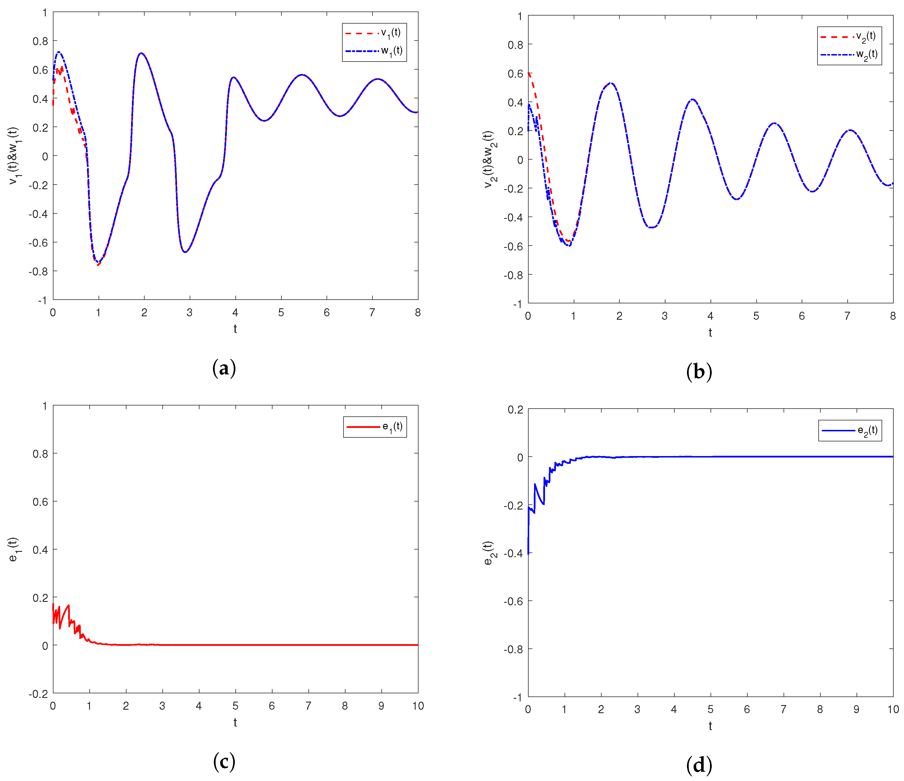
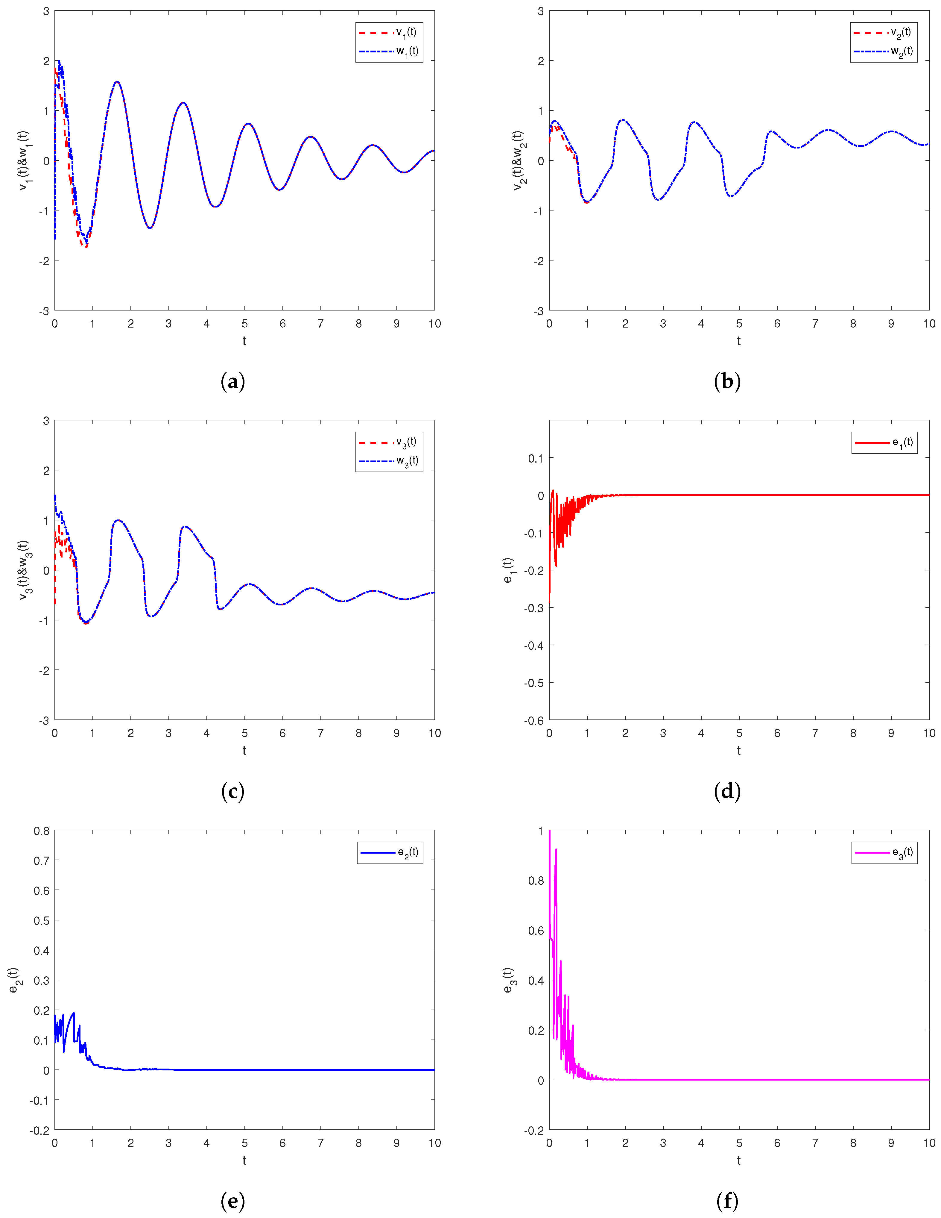
4. Numerical Simulations

This section presents two simulation examples to demonstrate the applicability of the theoretical results obtained in the previous sections.

Example 1.

Take a two-dimensional fractional-order memristive system including the parameters below as the drive network.

$$\begin{array}{c}\hfill c_{11}\left(v_1\right)=\left\{\begin{array}{c}0.6,|v_1\left(t\right)|<1,\hfill \\ -0.8,|v_1\left(t\right)|>1,\hfill \end{array}\right.\hspace{1em}{c}_{12}\left(v_1\right)=\left\{\begin{array}{c}0.2,|v_1\left(t\right)|<1,\hfill \\ -0.3,|v_1\left(t\right)|>1,\hfill \end{array}\right.\end{array}$$

$$\begin{array}{c}\hfill c_{21}\left(v_2\right)=\left\{\begin{array}{c}0.5,|v_2\left(t\right)|<1,\hfill \\ -0.7,|v_2\left(t\right)|>1,\hfill \end{array}\right.\hspace{1em}{c}_{22}\left(v_2\right)=\left\{\begin{array}{c}0.1,|v_2\left(t\right)|<1,\hfill \\ -0.3,|v_2\left(t\right)|>1,\hfill \end{array}\right.\end{array}$$

$$\begin{array}{c}\hfill d_{11}^1\left(v_1\right)=\left\{\begin{array}{c}0.4,|v_1\left(t\right)|<1,\hfill \\ -0.4,|v_1\left(t\right)|>1,\hfill \end{array}\right.\hspace{1em}{d}_{12}^1\left(v_1\right)=\left\{\begin{array}{c}0.6,|v_1\left(t\right)|<1,\hfill \\ -0.6,|v_1\left(t\right)|>1,\hfill \end{array}\right.\end{array}$$

$$\begin{array}{c}\hfill d_{21}^1\left(v_2\right)=\left\{\begin{array}{c}0.7,|v_2\left(t\right)|<1,\hfill \\ -0.7,|v_2\left(t\right)|>1,\hfill \end{array}\right.\hspace{1em}{d}_{22}^1\left(v_2\right)=\left\{\begin{array}{c}0.3,|v_2\left(t\right)|<1,\hfill \\ -0.3,|v_2\left(t\right)|>1,\hfill \end{array}\right.\end{array}$$

$$\begin{array}{c}\hfill d_{11}^2\left(v_1\right)=\left\{\begin{array}{c}0.5,|v_1\left(t\right)|<1,\hfill \\ -0.5,|v_1\left(t\right)|>1,\hfill \end{array}\right.\hspace{1em}{d}_{12}^2\left(v_1\right)=\left\{\begin{array}{c}0.8,|v_1\left(t\right)|<1,\hfill \\ -0.8,|v_1\left(t\right)|>1,\hfill \end{array}\right.\end{array}$$

$$\begin{array}{c}\hfill d_{21}^2\left(v_2\right)=\left\{\begin{array}{c}0.7,|v_2\left(t\right)|<1,\hfill \\ -0.7,|v_2\left(t\right)|>1,\hfill \end{array}\right.\hspace{1em}{d}_{22}^2\left(v_2\right)=\left\{\begin{array}{c}0.9,|v_2\left(t\right)|<1,\hfill \\ -0.9,|v_2\left(t\right)|>1,\hfill \end{array}\right.\end{array}$$

$b_1=4$, $b_2=5$, $\mu =0.8$, ${\tau }_1=0.2$, ${\tau }_2=0.3$, $I_1=1$, and $I_2=2$. The non-delay and delayed feedback functions are selected as ${\beta }_1\left(v\right)={\beta }_2\left(v\right)={\gamma }_1\left(v\right)={\gamma }_2\left(v\right)=tanhv$. When ${\tilde{\beta }}_i={\tilde{\gamma }}_i=M_i={\overline{M}}_i=1(i=1,2)$, it is not difficult to validate that the function $tanhv$ is bounded and conforms to the Lipschitz condition, which means Assumption 1 and Assumption 2 hold. The parameters of the response network are consistent with those of the drive network. Let ${\varsigma }_i=0.5$, ${\alpha }_i=-0.2$, $\rho =0.78$, and $t_k-t_{k-1}=0.1$, then simple calculation gives that $\sqrt{2}{\displaystyle \sum _{m=1}^h}{max}_{1\le i\le n}\left({\displaystyle \sum _{j=1}^n}{d}_{ji}^{m^{*}}{\tilde{\gamma }}_i\right)=3.9598<4.1={min}_{1\le i\le n}\left[2(b_i+{\varsigma }_i)-{\displaystyle \sum _{j=1}^n}{c}_{ij}^{*}{\tilde{\beta }}_j-{\displaystyle \sum _{j=1}^n}{c}_{ji}^{*}{\tilde{\beta }}_i-{\displaystyle \sum _{m=1}^h\sum _{j=1}^n}{d}_{ij}^{m^{*}}{\tilde{\gamma }}_j\right]$, and $\left[\begin{array}{cc}-0.78I_n& E_n^T\\ E_n& -I_n\end{array}\right]\le 0$. Hence, one can easily find that all circumstances in Theorem 1 are fulfilled. The starting values of the master–slave networks are randomly selected within the interval $\left[01\right]$. Under the hybrid impulsive feedback control schemes, the state trajectories of master–slave systems (1) and (13) are given in Figure 1a,b and the corresponding synchronization errors can be seen in Figure 1c,d. The experimental results show that master–slave systems (1) and (13) can achieve drive–response synchronization.

Example 2.

Take a three-dimensional fractional-order memristive system including the parameters below as the drive network.

$$\begin{array}{c}\hfill c_{11}\left(v_1\right)=\left\{\begin{array}{c}2.0,|v_1\left(t\right)|<1,\hfill \\ -2.0,|v_1\left(t\right)|>1,\hfill \end{array}\right.\hspace{1em}{c}_{12}\left(v_1\right)=\left\{\begin{array}{c}-1.2,|v_1\left(t\right)|<1,\hfill \\ 1.2,|v_1\left(t\right)|>1,\hfill \end{array}\right.\hspace{1em}{c}_{13}\left(v_1\right)=\left\{\begin{array}{c}1.0,|v_1\left(t\right)|<1,\hfill \\ -1.0,|v_1\left(t\right)|>1,\hfill \end{array}\right.\end{array}$$

$$\begin{array}{c}\hfill c_{21}\left(v_2\right)=\left\{\begin{array}{c}1.8,|v_2\left(t\right)|<1,\hfill \\ -1.8,|v_2\left(t\right)|>1,\hfill \end{array}\right.\hspace{1em}{c}_{22}\left(v_2\right)=\left\{\begin{array}{c}1.6,|v_2\left(t\right)|<1,\hfill \\ -1.6,|v_2\left(t\right)|>1,\hfill \end{array}\right.\hspace{1em}{c}_{23}\left(v_2\right)=\left\{\begin{array}{c}1.1,|v_2\left(t\right)|<1,\hfill \\ -1.1,|v_2\left(t\right)|>1,\hfill \end{array}\right.\end{array}$$

$$\begin{array}{c}\hfill c_{31}\left(v_3\right)=\left\{\begin{array}{c}1.5,|v_3\left(t\right)|<1,\hfill \\ -1.5,|v_3\left(t\right)|>1,\hfill \end{array}\right.\hspace{1em}{c}_{32}\left(v_3\right)=\left\{\begin{array}{c}2.5,|v_3\left(t\right)|<1,\hfill \\ -2.5,|v_3\left(t\right)|>1,\hfill \end{array}\right.\hspace{1em}{c}_{33}\left(v_3\right)=\left\{\begin{array}{c}2.0,|v_3\left(t\right)|<1,\hfill \\ -2.0,|v_3\left(t\right)|>1,\hfill \end{array}\right.\end{array}$$

$$\begin{array}{c}\hfill d_{11}^1\left(v_1\right)=\left\{\begin{array}{c}1.5,|v_1\left(t\right)|<1,\hfill \\ -1.5,|v_1\left(t\right)|>1,\hfill \end{array}\right.\hspace{1em}{d}_{12}^1\left(v_1\right)=\left\{\begin{array}{c}1.0,|v_1\left(t\right)|<1,\hfill \\ -1.0,|v_1\left(t\right)|>1,\hfill \end{array}\right.\hspace{1em}{d}_{13}^1\left(v_1\right)=\left\{\begin{array}{c}0.5,|v_1\left(t\right)|<1,\hfill \\ -0.5,|v_1\left(t\right)|>1,\hfill \end{array}\right.\end{array}$$

$$\begin{array}{c}\hfill d_{21}^1\left(v_2\right)=\left\{\begin{array}{c}1.5,|v_2\left(t\right)|<1,\hfill \\ -1.5,|v_2\left(t\right)|>1,\hfill \end{array}\right.\hspace{1em}{d}_{22}^1\left(v_2\right)=\left\{\begin{array}{c}2.0,|v_2\left(t\right)|<1,\hfill \\ -2.0,|v_2\left(t\right)|>1,\hfill \end{array}\right.\hspace{1em}{d}_{23}^1\left(v_2\right)=\left\{\begin{array}{c}1.5,|v_2\left(t\right)|<1,\hfill \\ -1.5,|v_2\left(t\right)|>1,\hfill \end{array}\right.\end{array}$$

$$\begin{array}{c}\hfill d_{31}^1\left(v_3\right)=\left\{\begin{array}{c}1.0,|v_3\left(t\right)|<1,\hfill \\ -1.0,|v_3\left(t\right)|>1,\hfill \end{array}\right.\hspace{1em}{d}_{32}^1\left(v_3\right)=\left\{\begin{array}{c}2.0,|v_3\left(t\right)|<1,\hfill \\ -2.0,|v_3\left(t\right)|>1,\hfill \end{array}\right.\hspace{1em}{d}_{33}^1\left(v_3\right)=\left\{\begin{array}{c}0.5,|v_3\left(t\right)|<1,\hfill \\ -0.5,|v_3\left(t\right)|>1,\hfill \end{array}\right.\end{array}$$

$$\begin{array}{c}\hfill d_{11}^2\left(v_1\right)=\left\{\begin{array}{c}0.5,|v_1\left(t\right)|<1,\hfill \\ -0.5,|v_1\left(t\right)|>1,\hfill \end{array}\right.\hspace{1em}{d}_{12}^2\left(v_1\right)=\left\{\begin{array}{c}0.8,|v_1\left(t\right)|<1,\hfill \\ -0.8,|v_1\left(t\right)|>1,\hfill \end{array}\right.\hspace{1em}{d}_{13}^2\left(v_1\right)=\left\{\begin{array}{c}0.6,|v_1\left(t\right)|<1,\hfill \\ -0.6,|v_1\left(t\right)|>1,\hfill \end{array}\right.\end{array}$$

$$\begin{array}{c}\hfill d_{21}^2\left(v_2\right)=\left\{\begin{array}{c}1.0,|v_2\left(t\right)|<1,\hfill \\ -1.0,|v_2\left(t\right)|>1,\hfill \end{array}\right.\hspace{1em}{d}_{22}^2\left(v_2\right)=\left\{\begin{array}{c}1.6,|v_2\left(t\right)|<1,\hfill \\ -1.6,|v_2\left(t\right)|>1,\hfill \end{array}\right.\hspace{1em}{d}_{23}^2\left(v_2\right)=\left\{\begin{array}{c}0.6,|v_2\left(t\right)|<1,\hfill \\ -0.6,|v_2\left(t\right)|>1,\hfill \end{array}\right.\end{array}$$

$$\begin{array}{c}\hfill d_{31}^2\left(v_3\right)=\left\{\begin{array}{c}0.8,|v_3\left(t\right)|<1,\hfill \\ -0.8,|v_3\left(t\right)|>1,\hfill \end{array}\right.\hspace{1em}{d}_{32}^2\left(v_3\right)=\left\{\begin{array}{c}1.2,|v_3\left(t\right)|<1,\hfill \\ -1.2,|v_3\left(t\right)|>1,\hfill \end{array}\right.\hspace{1em}{d}_{33}^2\left(v_3\right)=\left\{\begin{array}{c}0.4,|v_3\left(t\right)|<1,\hfill \\ -0.4,|v_3\left(t\right)|>1,\hfill \end{array}\right.\end{array}$$

$$\begin{array}{c}\hfill d_{11}^3\left(v_1\right)=\left\{\begin{array}{c}0.8,|v_1\left(t\right)|<1,\hfill \\ -0.8,|v_1\left(t\right)|>1,\hfill \end{array}\right.\hspace{1em}{d}_{12}^3\left(v_1\right)=\left\{\begin{array}{c}1.0,|v_1\left(t\right)|<1,\hfill \\ -1.0,|v_1\left(t\right)|>1,\hfill \end{array}\right.\hspace{1em}{d}_{13}^3\left(v_1\right)=\left\{\begin{array}{c}0.4,|v_1\left(t\right)|<1,\hfill \\ -0.4,|v_1\left(t\right)|>1,\hfill \end{array}\right.\end{array}$$

$$\begin{array}{c}\hfill d_{21}^3\left(v_2\right)=\left\{\begin{array}{c}1.5,|v_2\left(t\right)|<1,\hfill \\ -1.5,|v_2\left(t\right)|>1,\hfill \end{array}\right.\hspace{1em}{d}_{22}^3\left(v_2\right)=\left\{\begin{array}{c}1.2,|v_2\left(t\right)|<1,\hfill \\ -1.2,|v_2\left(t\right)|>1,\hfill \end{array}\right.\hspace{1em}{d}_{23}^3\left(v_2\right)=\left\{\begin{array}{c}0.5,|v_2\left(t\right)|<1,\hfill \\ -0.5,|v_2\left(t\right)|>1,\hfill \end{array}\right.\end{array}$$

$$\begin{array}{c}\hfill d_{31}^3\left(v_3\right)=\left\{\begin{array}{c}1.1,|v_3\left(t\right)|<1,\hfill \\ -1.1,|v_3\left(t\right)|>1,\hfill \end{array}\right.\hspace{1em}{d}_{32}^3\left(v_3\right)=\left\{\begin{array}{c}1.0,|v_3\left(t\right)|<1,\hfill \\ -1.0,|v_3\left(t\right)|>1,\hfill \end{array}\right.\hspace{1em}{d}_{33}^3\left(v_3\right)=\left\{\begin{array}{c}0.7,|v_3\left(t\right)|<1,\hfill \\ -0.7,|v_3\left(t\right)|>1,\hfill \end{array}\right.\end{array}$$

$b_1=4$, $b_2=5$, $b_3=6$, $\mu =0.8$, ${\tau }_1=0.05$, ${\tau }_2=0.10$, ${\tau }_3=0.12$. The non-delay feedback function is the same as Example 1 and the delayed feedback function is selected as ${\gamma }_1\left(v\right)={\gamma }_2\left(v\right)={\gamma }_3\left(v\right)=\frac{1}{2}\left(\right|1+v|-|1-v\left|\right)$. We can conclude that $|{\gamma }_1\left(v\right)| = |{\gamma }_2\left(v\right)| = |{\gamma }_3\left(v\right)|\le 1$ and ${\dot{\gamma }}_1\left(v\right)={\dot{\gamma }}_2\left(v\right)={\dot{\gamma }}_3\left(v\right)=\frac{1}{2}[\mathrm{sign}(1+v)-\mathrm{sign}(1-v)]$. Let ${\tilde{\gamma }}_i={\overline{M}}_i=1$, then one can easily find that the function ${\gamma }_i\left(v\right)$ conforms to Assumptions 1 and 2. The parameters of the response network are consistent with those of the drive network. Let ${\varsigma }_i=15$, ${\alpha }_i=-2.1$, $\rho =1.3$, $\xi =1.1$, and $t_k-t_{k-1}=0.4$, then simple calculation gives ${min}_{1\le i\le n}\left[2(b_i+{\varsigma }_i)-{\displaystyle \sum _{j=1}^n}{c}_{ij}^{*}{\tilde{\beta }}_j-{\displaystyle \sum _{j=1}^n}{c}_{ji}^{*}{\tilde{\beta }}_i-{\displaystyle \sum _{m=1}^h}{\displaystyle \sum _{j=1}^n}{d}_{ij}^{m^{*}}{\tilde{\gamma }}_j\right]=18.8$, ${max}_{1\le i\le n}\left({\displaystyle \sum _{j=1}^n}{d}_{ji}^{1^{*}}{\tilde{\gamma }}_i\right)=5$, ${max}_{1\le i\le n}\left({\displaystyle \sum _{j=1}^n}{d}_{ji}^{2^{*}}{\tilde{\gamma }}_i\right)=3.6$, ${max}_{1\le i\le n}\left({\displaystyle \sum _{j=1}^n}{d}_{ji}^{3^{*}}{\tilde{\gamma }}_i\right)=3.4$, $\eta ={\lambda }_0-{\displaystyle \sum _{m=1}^h}{\lambda }_m{F}_m=0.8$, $\rho E_{\mu }[-\eta {(t_k-t_{k-1})}^{\mu }]=0.8763<0.9091={\xi }^{-1}$, and $\left[\begin{array}{cc}-1.3I_n& E_n^T\\ E_n& -I_n\end{array}\right]\le 0$. Thus, it can be observed that all the conditions in Theorem 2 are satisfied. The initial values of the master–slave networks are randomly chosen from the interval $[-22]$. The time evolution of the state trajectories of the master–slave systems (1) and (13) are depicted in Figure 2a,b, while Figure 2c,d shows the corresponding synchronization errors. The experimental results demonstrate that the proposed control schemes can achieve drive–response synchronization of the master–slave systems (1) and (13) when the parameters satisfy the requirements of Theorem 2.

5. Conclusions

This study investigates the drive–response synchronization of a class of fractional-order multi-link memristive neural networks (FMMNN), where multiple time delays and impulsive effects are considered in the response system. A more generalized fractional-order comparison principle that includes delays and impulses is proposed to overcome the stability issues induced by delays. By employing hybrid impulsive feedback control techniques, novel synchronization criteria are obtained to ensure the synchronization of master–slave neural networks. The derived criteria depend on impulsive intervals, fractional order, impulsive and feedback gains. Notably, the scope of impulses considered in this study is wider than that of previous works, enhancing the practicality of our hybrid impulsive control method. Finally, numerical examples are presented to validate our theoretical findings.

References

1. Adhikari, S.P.; Yang, C.; Kim, H.; Chua, L.O. Memristor bridge synapse-based neural network and its learning. IEEE Transacations Neural Netw. Learn. Syst. 2012, 23, 1426–1435. [Google Scholar] [CrossRef] [PubMed]
2. Pershin, Y.V.; di Ventra, M. On the validity of memristor modeling in the neural network literature. Neural Netw. 2020, 121, 52–56. [Google Scholar] [CrossRef] [PubMed]
3. Ding, K.; Zhu, Q.X. A note on sampled-data synchronization of memristor networks subject to actuator failures and two different activations. IEEE Trans. Circuits Syst. II Express Briefs 2021, 68, 2097–2101. [Google Scholar] [CrossRef]
4. Wang, X.; Park, J.H.; Zhong, S.; Yang, H. A switched operation approach to sampled-data control stabilization of fuzzy memristive neural networks with time-varying delay. IEEE Transacations Neural Netw. Learn. Syst. 2020, 31, 891–900. [Google Scholar] [CrossRef]
5. Zhou, C.; Wang, C.; Yao, W.; Lin, H. Observer-based synchronization of memristive neural networks under dos attacks and actuator saturation and its application to image encryptiong. Appl. Math. Comput. 2022, 425, 127080. [Google Scholar]
6. Cheng, J.; Lin, A.; Cao, J.; Qiu, J.; Qi, W. Protocol-based fault detection for discrete-time memristive neural networks with effect. Inf. Sci. 2022, 615, 118–135. [Google Scholar] [CrossRef]
7. Lu, J.; Kurths, J.; Cao, J.; Mahdavi, N.; Huang, C. Synchronization control for nonlinear stochastic dynamical networks: Pinning impulsive strategy. IEEE Trans. Netw. Sci. Eng. 2012, 23, 285–292. [Google Scholar]
8. Jiang, C.; Tang, Z.; Park, J.H.; Xiong, N.N. Matrix measure-based projective synchronization on coupled neural networks with clustering treess. IEEE Trans. Cybern. 2023, 53, 1222–1234. [Google Scholar] [CrossRef]
9. Bao, H.B.; Park, J.H.; Cao, J.D. Exponential synchronization of coupled stochastic memristor-based neural networks with time-varying probabilistic delay coupling and impulsive delay. IEEE Transacations Neural Netw. Learn. Syst. 2016, 27, 190–201. [Google Scholar] [CrossRef]
10. Li, X.; Zhang, W.; Fang, J.A.; Li, H. Finite-time synchronization of memristive neural networks with discontinuous activation functions and mixed time-varying delays. Neurocomputing 2019, 340, 99–109. [Google Scholar] [CrossRef]
11. Yu, T.H.; Cao, J.D.; Rutkowski, L.; Luo, Y.P. Finite-time synchronization of complex-valued memristive-based neural networks via hybrid controls. IEEE Trans. Neural Netw. Learn. Syst. 2022, 33, 3938–3947. [Google Scholar] [CrossRef]
12. Yang, S.F.; Guo, Z.Y.; Wang, J. Robust synchronization of multiple memristive neural networks with uncertain parameters via nonlinear coupling. IEEE Trans. Syst. Man Cybern. Syst. 2015, 45, 1077–1086. [Google Scholar] [CrossRef]
13. Zhang, S.; Yang, Y.Q.; Sui, X.; Xu, X.Y. Finite-time synchronization of memristive neural networks with parameter uncertainties via aperiodically intermittent adjustment. Phys. A 2019, 534, 122258. [Google Scholar] [CrossRef]
14. Alsaedi, A.; Cao, J.; Ahmad, B.; Alshehri, A.; Tan, X. Synchronization of master–slave memristive neural networks via fuzzy output-based adaptive strategy. Chaos Solitons Fractals 2022, 158, 112095. [Google Scholar] [CrossRef]
15. Ding, K.; Zhu, Q.X. Intermittent quasi-synchronization criteria of chaotic delayed neural networks with parameter mismatches and stochastic perturbation mismatches via Razumikhin-type approach. Neurocomputing 2019, 356, 314–324. [Google Scholar] [CrossRef]
16. Liu, L.R.; Bao, H.B. Event-triggered impulsive synchronization of coupled delayed memristive neural networks under dynamic and static conditions. Neurocomputing 2022, 504, 109–122. [Google Scholar] [CrossRef]
17. Wang, F.; Zheng, Z.W.; Yang, Y.Q. Quasi-synchronization of heterogenous fractional-order dynamical networks with time-varying delay via distributed impulsive control. Chaos Solitons Fractals 2021, 142, 110465. [Google Scholar] [CrossRef]
18. Podlubny, I. Fractional Differential Equations; Academic Press: New York, NY, USA, 1999. [Google Scholar]
19. Srivastava, H.M. Some parametric and argument variations of the operators of fractional calculus and related special functions and integral transformations. J. Nonlinear Convex Anal. 2021, 22, 1501–1520. [Google Scholar]
20. Srivastava, H.M. An introductory overview of fractional-calculus operators based upon the fox-wright and related higher transcendental functions. J. Adv. Engrg. Comput. 2021, 5, 135–166. [Google Scholar] [CrossRef]
21. Srivastava, H.M. Fractional-order derivatives and integrals: Introductory overview and recent developments. Kyungpook Math. J. 2020, 60, 73–116. [Google Scholar]
22. Li, Y.R.; Wang, F.; Zheng, Z.W. Adaptive synchronization-based approach for finite-time parameters identification of genetic regulatory networks. Neural Process. Lett. 2022, 54, 3141–3156. [Google Scholar] [CrossRef]
23. Wang, H.; Yu, Y.; Wen, G.; Zhang, S.; Yu, J. Global stability analysis of fractional-order Hopfield neural networks with time delay. Neurocomputing 2015, 154, 15–23. [Google Scholar] [CrossRef]
24. Li, H.L.; Jiang, Y.L.; Wang, Z.; Zhang, L.; Teng, Z. Global Mittag–Leffler stability of coupled system of fractional-order differential equations on network. Appl. Math. Comput. 2015, 270, 269–277. [Google Scholar] [CrossRef]
25. Chen, J.J.; Zeng, Z.G.; Jiang, P. Global Mittag–Leffler stability and synchronization of memristor-based fractional-order neural networks. Neural Netw. 2014, 51, 1–8. [Google Scholar] [CrossRef]
26. Bao, H.B.; Cao, J.D. Projective synchronization of fractional-order memristor-based neural networks. Neural Netw. 2015, 63, 1–9. [Google Scholar] [CrossRef]
27. Jiang, M.H.; Wang, S.T.; Mei, J.; Shen, Y.J. Finite-time synchronization control of a class of memristor-based recurrent neural networks. Neural Netw. 2015, 63, 133–140. [Google Scholar] [CrossRef] [PubMed]
28. Chen, L.; Wu, R.; Cao, J.; Liu, J.B. Stability and synchronization of memristor-based fractional-order delayed neural networks. Neural Netw. 2015, 71, 37–44. [Google Scholar] [CrossRef]
29. Velmurugan, G.; Rakkiyappan, R. Hybrid projective synchronization of fractional-order memristor-based neural networks with time delays. Nonlinear Dyn. 2016, 83, 419–432. [Google Scholar] [CrossRef]
30. Velmurugan, G.; Rakkiyappan, R.; Cao, J.D. Finite-time synchronization of fractional-order memristor-based neural networks with time delays. Neural Netw. 2016, 73, 36–46. [Google Scholar] [CrossRef]
31. Chen, L.P.; Cao, J.D.; Wu, R.C.; Machado, J.A.T.; Lopes, A.M. Stability and synchronization of fractional-order memristive neural networks with multiple delays. Neural Netw. 2017, 94, 76–85. [Google Scholar] [CrossRef]
32. Huang, X.; Fan, Y.; Jia, J.; Wang, Z.; Li, Y. Quasi-synchronisation of fractional-order memristor-based neural networks with parameter mismatches. IET Control. Theory Appl. 2017, 11, 2317–2327. [Google Scholar] [CrossRef]
33. Du, F.F.; Lu, J.G. New criterion for finite-time synchronization of fractional order memristor-based neural networks with time delay. Appl. Math. Comput. 2021, 389, 125616. [Google Scholar] [CrossRef]
34. Filippov, A. Differential Equations with Discontinuous Right-Hand Side; Mathematics and Its Applications (Soviet Series); Kluwer Academic: Boston, MA, USA, 1988. [Google Scholar]
35. Liu, P.; Zeng, Z.; Wang, J. Multiple Mittag–Leffler stability of fractional-order recurrent neural networks. IEEE Trans. Syst. Man Cybern. Syst. 2017, 47, 2279–2288. [Google Scholar] [CrossRef]
36. Aguila-Camacho, N.; Duarte-Mermoud, M.; Gallegos, J. Lyapunov functions for fractional orer systems. Commun. Nonlinear Sci. Numer. Simul. 2014, 19, 2951–2957. [Google Scholar] [CrossRef]
37. Boyd, S.; Ghaoui, L.E.; Feron, E.; Balakrishnan, V. Linear Matrix Inequalities in System and Control Theory; SIAM: Philadelphia, PA, USA, 1994. [Google Scholar]
Figure 1. The state trajectories and error signals in master–slave systems (1) and (13) under hybrid impulsive feedback control in Example 1. (a) v 1 ( t ) & w 1 ( t ) ; (b) v 2 ( t ) & w 2 ( t ) ; (c) e 1 ( t ) ; (d) e 2 ( t ) .
Fractalfract 07 00495 g001
Figure 2. The state trajectories and error signals in master–slave systems (1) and (13) under hybrid impulsive feedback control in Example 2. (a) v 1 ( t ) & w 1 ( t ) ; (b) v 2 ( t ) & w 2 ( t ) ; (c) v 3 ( t ) & w 3 ( t ) ; (d) e 1 ( t ) ; (e) e 2 ( t ) ; (f) e 3 ( t ) .
Fractalfract 07 00495 g002
Disclaimer/Publisher’s Note: The statements, opinions and data contained in all publications are solely those of the individual author(s) and contributor(s) and not of MDPI and/or the editor(s). MDPI and/or the editor(s) disclaim responsibility for any injury to people or property resulting from any ideas, methods, instructions or products referred to in the content.