
Approximate Controllability of Ψ-Hilfer Fractional Neutral Differential Equation with Infinite Delay
 , , , and
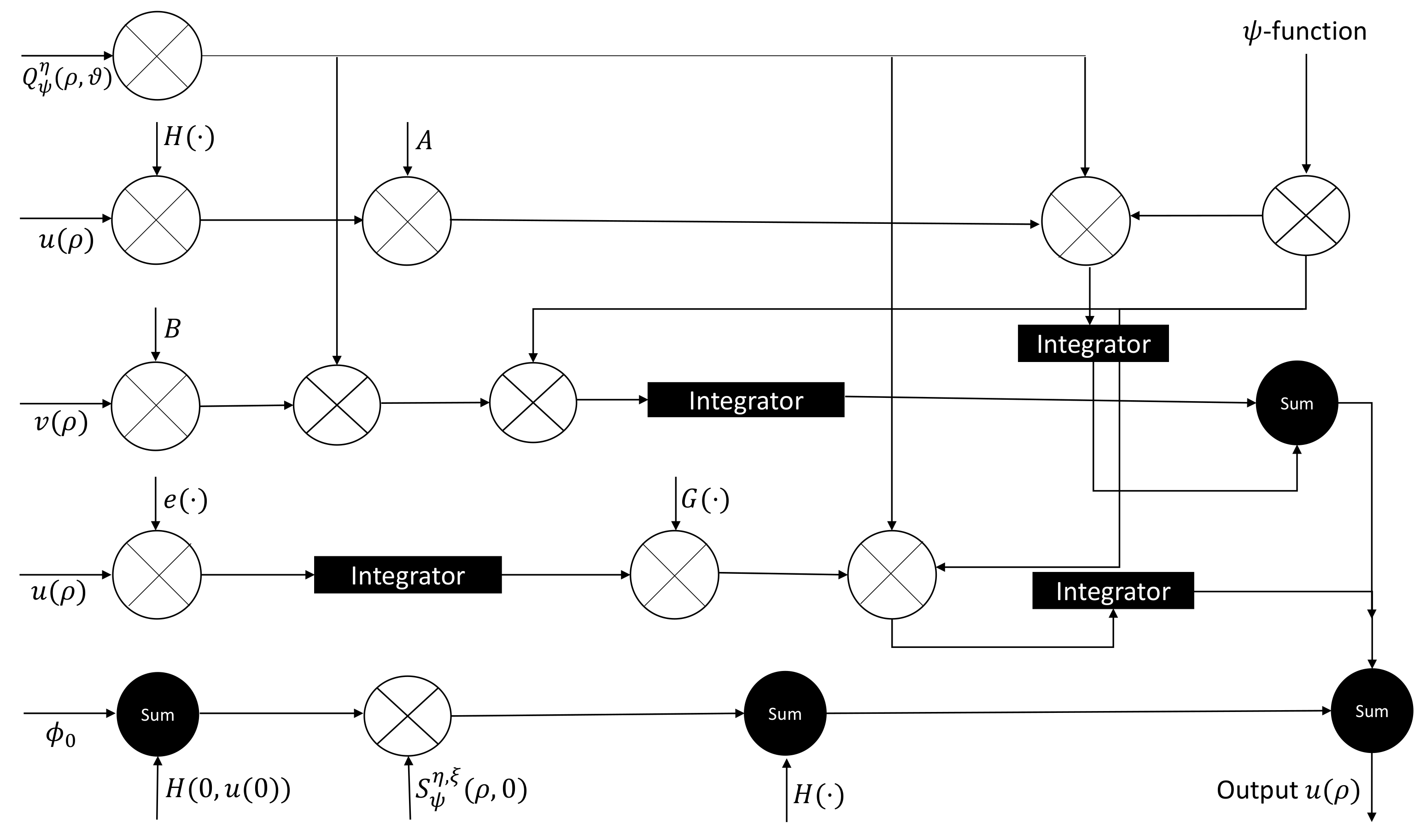
Abstract
:1. Introduction
2. Preliminaries
- (ci)
- is closed and ;
- (cii)
- is the resolvent set of containing and , we writewhere .
- 1.
- ;
- 2.
- , for ;
- 3.
- .
- (a)
- For any , and are bounded linear operators withwhere and for all .
- (b)
- The operators, and , are strongly continuous for all ; thus, we write
- (c)
- If is a compact operator , then and are compact for all .
- (d)
- If and are the compact strongly continuous semigroup of bounded linear operators for , then and are continuous in the uniform operator topology.
- (H1)
- is the -semigroup, such that .
- (H2)
- For , , are continuous functions, and for each , and are strongly measurable.
- (H3)
- There exists an increasing function and , such that for all , and ∃ a constant , then
- (H4)
- There exists a constant , such that: for all .
- (H5)
- The function is continuous, and there exists for any is strongly measurable, there exists such that:and there exists a constant such that:
3. Approximate Controllability
4. Application
4.1. Application 1
4.2. Application 2
- Product modulator 1 accepts the input and produces the output .
- Product modulator 2 accepts the input and and gives out put .
- Product modulator 3 accepts the input and produces the output .
- Product modulator 4 accepts the input and -function, and obtains the output .
- Product modulator 5 accepts the input and , and produces the output .
- Product modulator 6 accepts the input and , and gives the output .
- Product modulator 7 accepts the input and , and gives the output over the period .
- The integrator executes the input and and produces the outputover the period of time .
- Product modulator 8 accepts the input and and gives the output .
- Product modulator 9 accepts and at time , and produces .
- The integrators execute the following value:, and produces the integral value over the period .Finally, we turn all outputs from the integrators to the summer network and the output of is obtained; it is bounded and approximately controllable.
5. Conclusions
Author Contributions
Funding
Institutional Review Board Statement
Informed Consent Statement
Data Availability Statement
Acknowledgments
Conflicts of Interest
Abbreviations
| Hilfer Fractional Derivative | |
| Hilfer Fractional Differential | |
| MNC | Measure of Noncompactness. |
References
- Agarwal, R.P.; Lakshmikantham, V.; Nieto, J.J. On the concept of solution for fractional differential equations with uncertainty. Nonlinear Anal. 2010, 72, 2859–2862. [Google Scholar] [CrossRef]
- Ahmad, B.; Alsaedi, A.; Ntouyas, S.K.J.; Tariboon, J. Hadamard-Type Fractional Differential Equations, Inclusions and Inequalities; Springer International Publishing AG: Cham, Switzerland, 2017. [Google Scholar]
- Gu, H.; Trujillo, J.J. Existence of integral solution for evolution equation with Hilfer fractional derivative. Appl. Math. Comput. 2015, 257, 344–354. [Google Scholar]
- Hilfer, R. Application of Fractional Calculus in Physics; World Scientific: Singapore, 2000. [Google Scholar]
- Lakshmikantham, V.; Vatsala, A.S. Basic Theory of Fractional Differential Equations. Nonlinear Anal. Theory Methods Appl. 2008, 69, 2677–2682. [Google Scholar] [CrossRef]
- Miller, K.S.; Ross, B. An Introduction to the Fractional Calculus and Differential Equations; John Wiley: New York, NY, USA, 1993. [Google Scholar]
- Yang, M.; Wang, Q. Existence of mild solutions for a class of Hilfer fractional evolution equations with nonlocal conditions. Fract. Calc. Appl. Anal. 2017, 20, 679–705. [Google Scholar] [CrossRef]
- Podlubny, I. Fractional Differential Equations; Academic Press: San Diego, CA, USA, 1999. [Google Scholar]
- Pazy, A. Semigroups of Linear Operators and Applications to Partial Differential Equations; Applied Mathematical Sciences; Springer: New York, NY, USA, 1983. [Google Scholar]
- Varun Bose, C.S.; Udhayakumar, R. A note on the existence of Hilfer fractional differential inclusions with almost sectorial operators. Math. Methods Appl. Sci. 2022, 45, 2530–2541. [Google Scholar] [CrossRef]
- Zhou, Y. Basic Theory of Fractional Differential Equations; World Scientific: Singapore, 2014. [Google Scholar]
- Zhou, Y. Fractional Evolution Equations and Inclusions: Analysis and Control; Elsevier: New York, NY, USA, 2015. [Google Scholar]
- Rajchakit, G. Switching design for the asymptotic stability and stabilization of nonlinear uncertain stochastic discrete-time systems. Int. J. Nonlinear Sci. Numer. Simul. 2013, 14, 33–44. [Google Scholar] [CrossRef]
- Rajchakit, G. Switching design for the robust stability of nonlinear uncertain stochastic switched discrete-time systems with interval time-varying delay. J. Comput. Anal. Appl. 2014, 16, 10–19. [Google Scholar]
- Balachandran, K.; Sakthivel, R. Controllability of integro-differential systems in Banach spaces. Appl. Math. Comput. 2001, 118, 63–71. [Google Scholar]
- Chang, Y.K. Controllability of impulsive differential systems with infinite delay in Banach spaces. Chaos Solitons Fractals 2007, 33, 1601–1609. [Google Scholar] [CrossRef]
- Dineshkumar, C.; Udhayakumar, R. New results concerning to approximate controllability of Hilfer fractional neutral stochastic delay integro-differential system. Numer. Methods Partial Differ. Equ. 2020, 38, 509–524. [Google Scholar] [CrossRef]
- Gokulakrishnan, V.; Srinivasan, R.; Syed Ali, M.; Rajchakit, G. Finite-time guaranteed cost control for stochastic nonlinear switched systems with time-varying delays and reaction-diffusion. Int. J. Comput. Math. 2023, 100, 1031–1051. [Google Scholar]
- Sundara, V.B.; Raja, R.; Agarwal, R.P.; Rajchakit, G. A novel controllability analysis of impulsive fractional linear time invariant systems with state delay and distributed delays in control. Discontinuity Nonlinearity Complex. 2018, 7, 275–290. [Google Scholar]
- Vadivoo, B.S.; Raja, R.; Seadawy, R.A.; Rajchakit, G. Nonlinear integro-differential equations with small unknown parameters: A controllability analysis problem. Math. Comput. Simul. 2019, 155, 15–26. [Google Scholar] [CrossRef]
- Ji, S.; Li, G.; Wang, M. Controllability of impulsive differential systems with nonlocal conditions. Appl. Math. Comput. 2011, 217, 6981–6989. [Google Scholar] [CrossRef]
- Sakthivel, R.; Ganesh, R.; Anthoni, S.M. Approximate controllability of fractional nonlinear differential inclusions. Appl. Math. Comput. 2013, 225, 708–717. [Google Scholar] [CrossRef]
- Sakthivel, R.; Ganesh, R.; Ren, Y.; Anthoni, S.M. Approximate controllability of nonlinear fractional dynamic systems. Commun. Nonlinear Sci. Numer. Simul. 2013, 18, 3498–3508. [Google Scholar] [CrossRef]
- Singh, V. Controllability of Hilfer fractional differential systems with non-dense domain. Numer. Funct. Anal. Optim. 2019, 40, 1572–1592. [Google Scholar] [CrossRef]
- Wang, J.R.; Fan, Z.; Zhou, Y. Nonlocal controllability of semilinear dynamic systems with fractional derivative in Banach spaces. J. Optim. Theory Appl. 2012, 154, 292–302. [Google Scholar] [CrossRef]
- Almeida, R. A Caputo fractional derivative of a function with respect to another function. Commun. Nonlinear Sci. Numer. Simul. 2017, 44, 460–481. [Google Scholar] [CrossRef] [Green Version]
- Sousa, J.V.C.; Oliveira, C. On the Ψ-Hilfer fractional derivative. Cummun. Nonlinear Sci. Numer. Simul. 2018, 60, 72–91. [Google Scholar] [CrossRef]
- Suechoei, A.; Sa Ngiamsunthorn, P. Existence uniqueness and stability of mild solution for semilinear Ψ-Caputo fractional evolution equations. Adv. Differ. Equ. 2020, 2020, 114. [Google Scholar] [CrossRef] [Green Version]
- Norouzi, F.; N’guerekata, G.M. Existence results to a Ψ-Hilfer neutral fractional evolution with infinite delay. Nonautonomous Dyn. Syst. 2021, 8, 101–124. [Google Scholar] [CrossRef]
- Dhayal, R.; Zhu, Q. Stability and controllability results of Ψ-Hilfer fractional integro-differential system under the influence of impulses. Chaos Solitons Fractals 2023, 168, 113105. [Google Scholar] [CrossRef]
- Jarad, F.; Abdeljawad, T. Generalized fractional derivative and Laplace transform. Discret. Contin. Dyn. Syst. Ser. S 2020, 13, 709–722. [Google Scholar] [CrossRef] [Green Version]
- Shu, X.B.; Wang, Q. The existence and uniqueness of mild solutions for fractional differential equations with nonlocal conditions of order 1 < α < 2. Comput. Math. Appl. 2012, 64, 2100–2110. [Google Scholar]
- Dineshkumar, C.; Udhayakumar, R.; Vijayakumar, V.; Nisar, K.S. A discussion on the approximate controllability of Hilfer fractional neutral stochastic integro-differential system. Chaos Solitons Fractals 2021, 142, 110472. [Google Scholar] [CrossRef]
- Chandra, A.; Chattopadhyay, S. Design of hardware efficient FIR filter: A review of the state of the art approaches. Eng. Sci. Technol. Int. J. 2016, 19, 212–226. [Google Scholar] [CrossRef] [Green Version]
- Zahoor, S.; Naseem, S. Design and implementation of an efficient FIR digital filter. Cogent Eng. 2017, 4, 1323373. [Google Scholar] [CrossRef]

Disclaimer/Publisher’s Note: The statements, opinions and data contained in all publications are solely those of the individual author(s) and contributor(s) and not of MDPI and/or the editor(s). MDPI and/or the editor(s) disclaim responsibility for any injury to people or property resulting from any ideas, methods, instructions or products referred to in the content. |
© 2023 by the authors. Licensee MDPI, Basel, Switzerland. This article is an open access article distributed under the terms and conditions of the Creative Commons Attribution (CC BY) license (https://creativecommons.org/licenses/by/4.0/).
Share and Cite
Varun Bose, C.S.; Udhayakumar, R.; Velmurugan, S.; Saradha, M.; Almarri, B. Approximate Controllability of Ψ-Hilfer Fractional Neutral Differential Equation with Infinite Delay. Fractal Fract. 2023, 7, 537. https://doi.org/10.3390/fractalfract7070537
Varun Bose CS, Udhayakumar R, Velmurugan S, Saradha M, Almarri B. Approximate Controllability of Ψ-Hilfer Fractional Neutral Differential Equation with Infinite Delay. Fractal and Fractional. 2023; 7(7):537. https://doi.org/10.3390/fractalfract7070537
Chicago/Turabian StyleVarun Bose, Chandrabose Sindhu, Ramalingam Udhayakumar, Subramanian Velmurugan, Madhrubootham Saradha, and Barakah Almarri. 2023. "Approximate Controllability of Ψ-Hilfer Fractional Neutral Differential Equation with Infinite Delay" Fractal and Fractional 7, no. 7: 537. https://doi.org/10.3390/fractalfract7070537