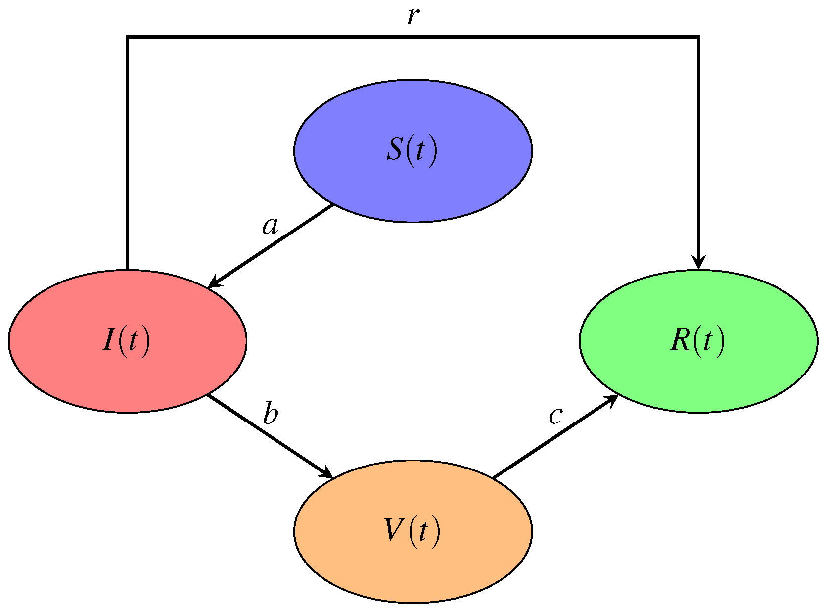
Figure 1.
Graphical representation of the SIVR model.
Figure 1.
Graphical representation of the SIVR model.
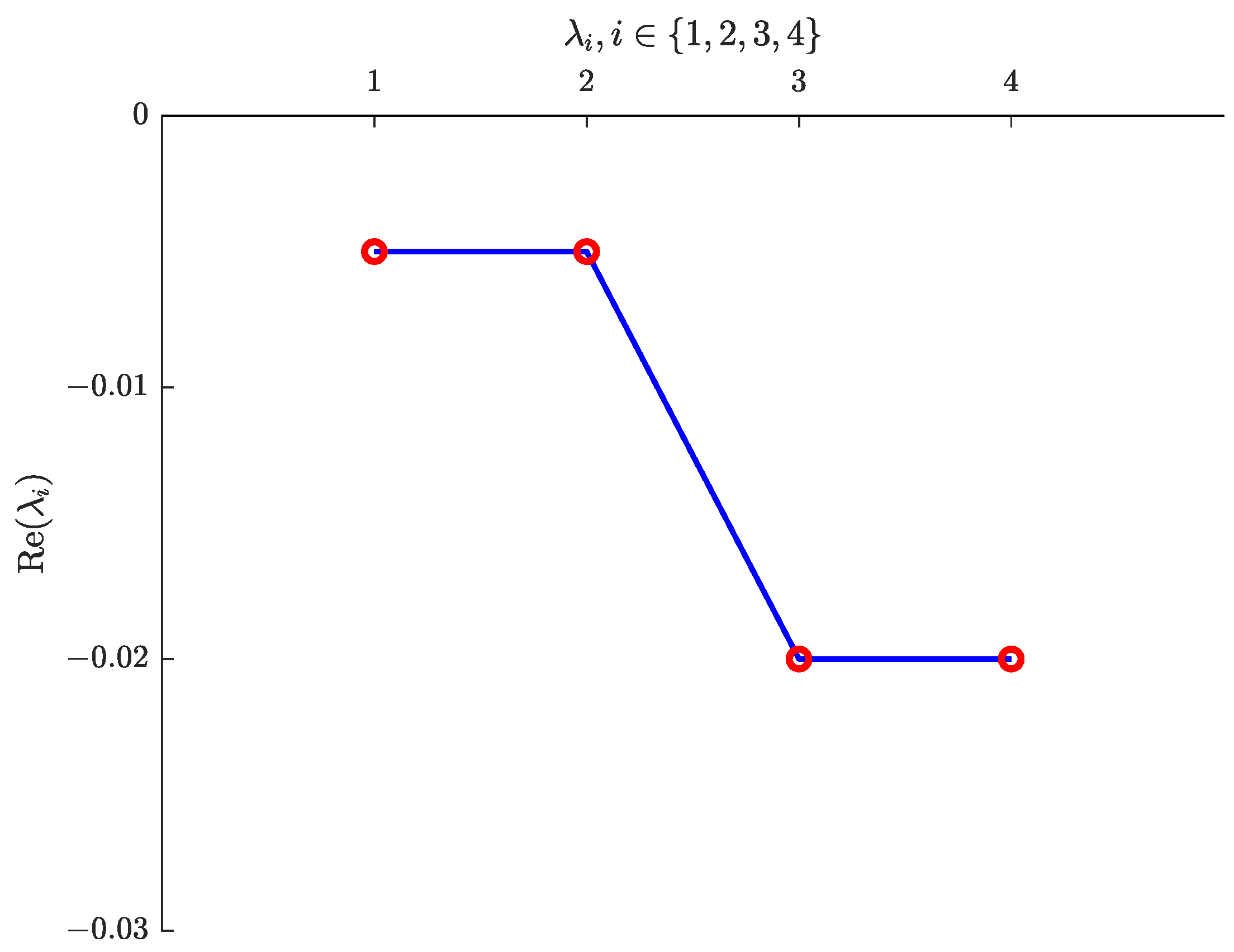
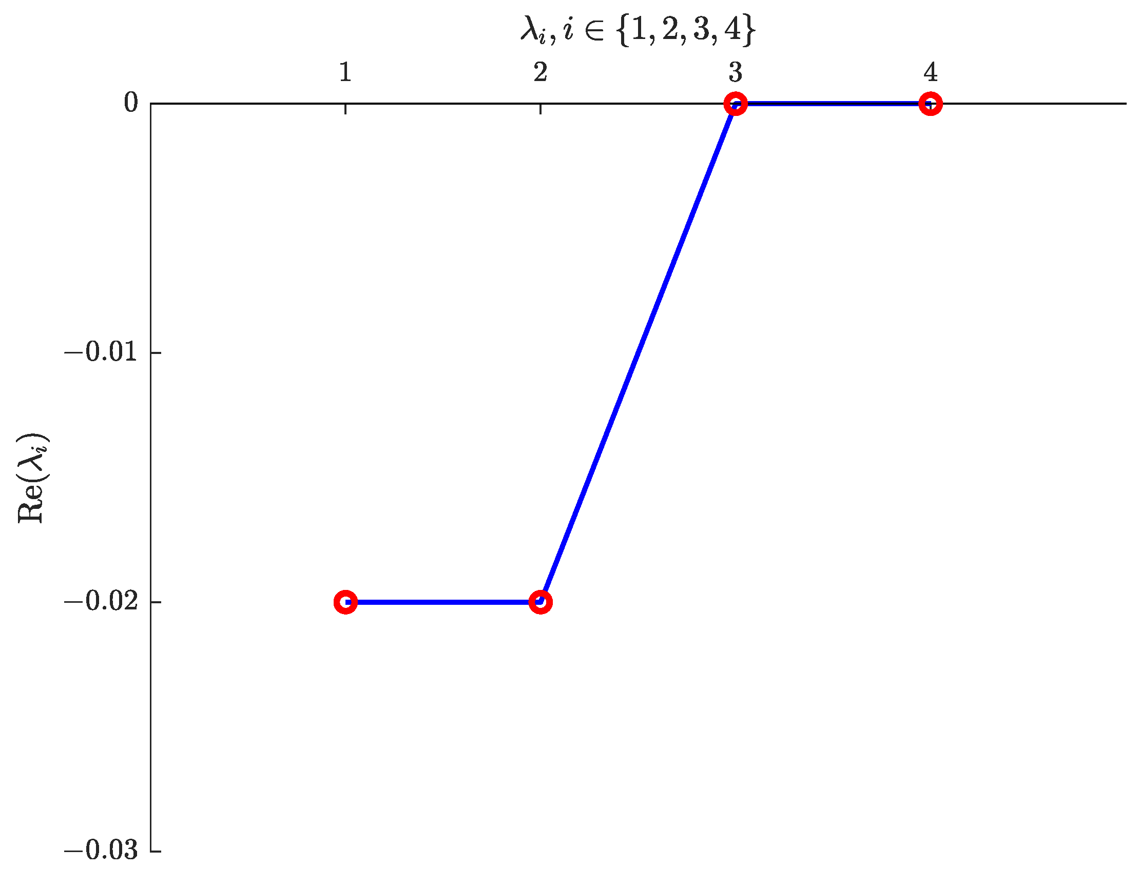
Figure 2.
Negative real parts of the eigenvalues of J.
Figure 2.
Negative real parts of the eigenvalues of J.
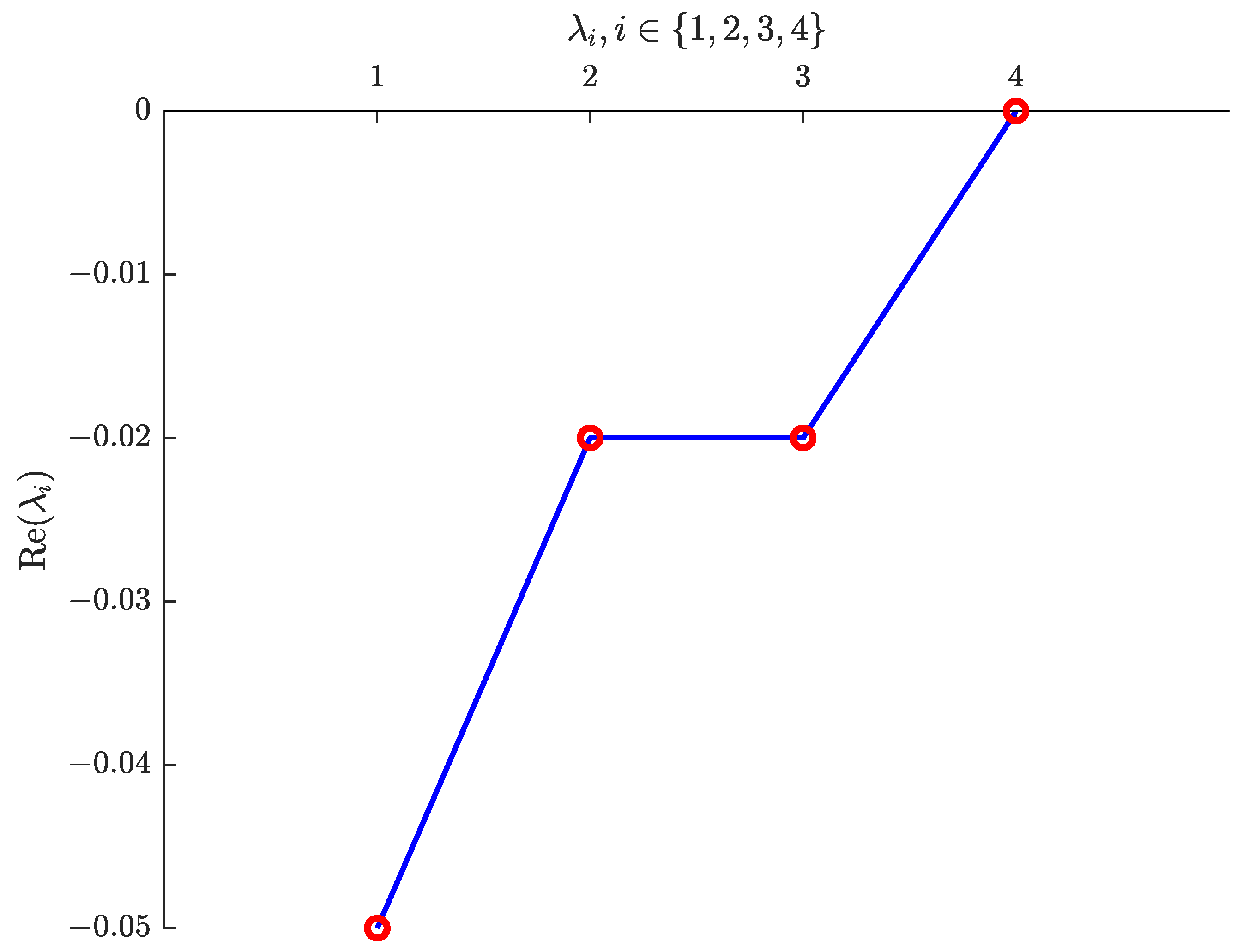
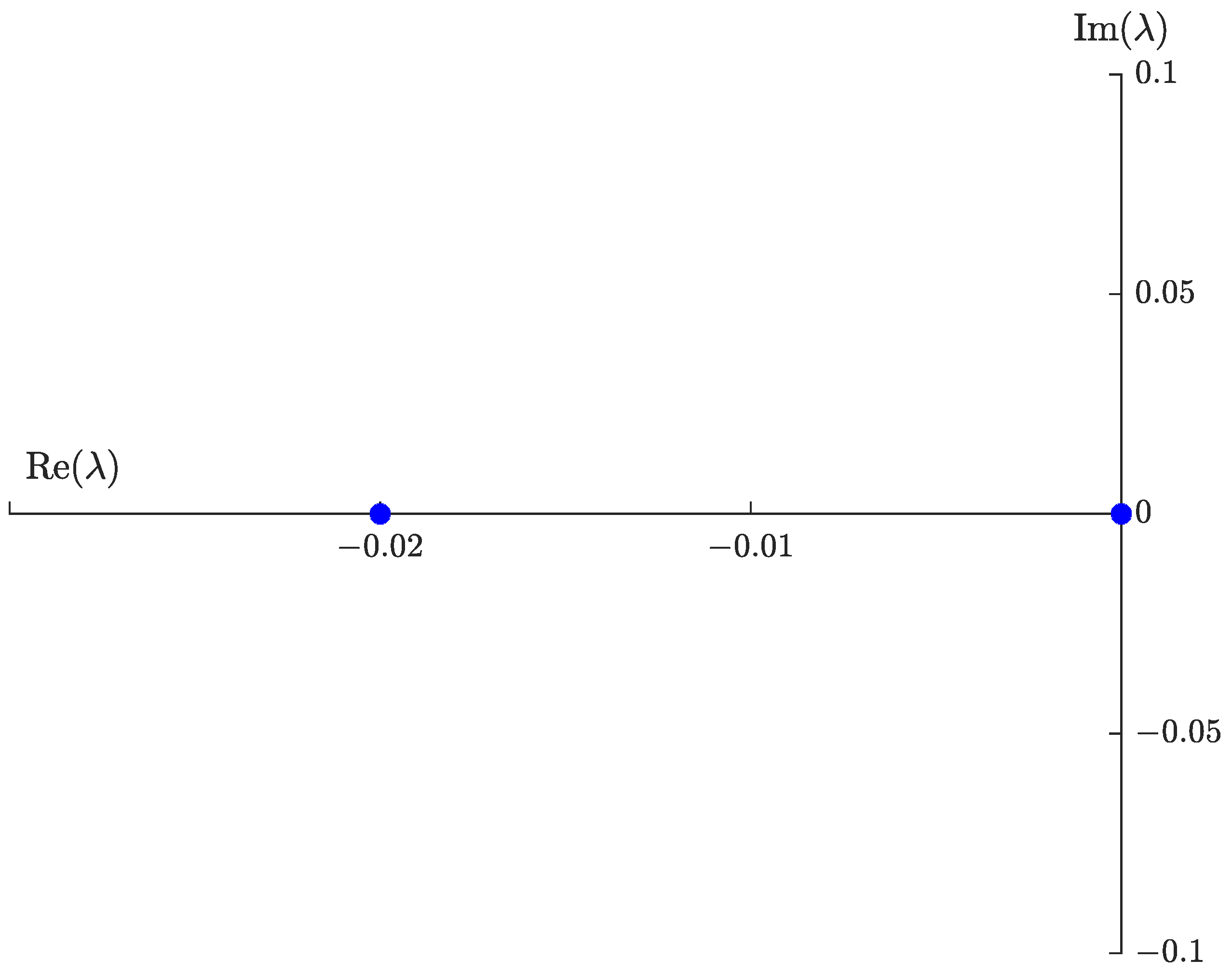
Figure 3.
Real and imaginary parts of the eigenvalues of J.
Figure 3.
Real and imaginary parts of the eigenvalues of J.
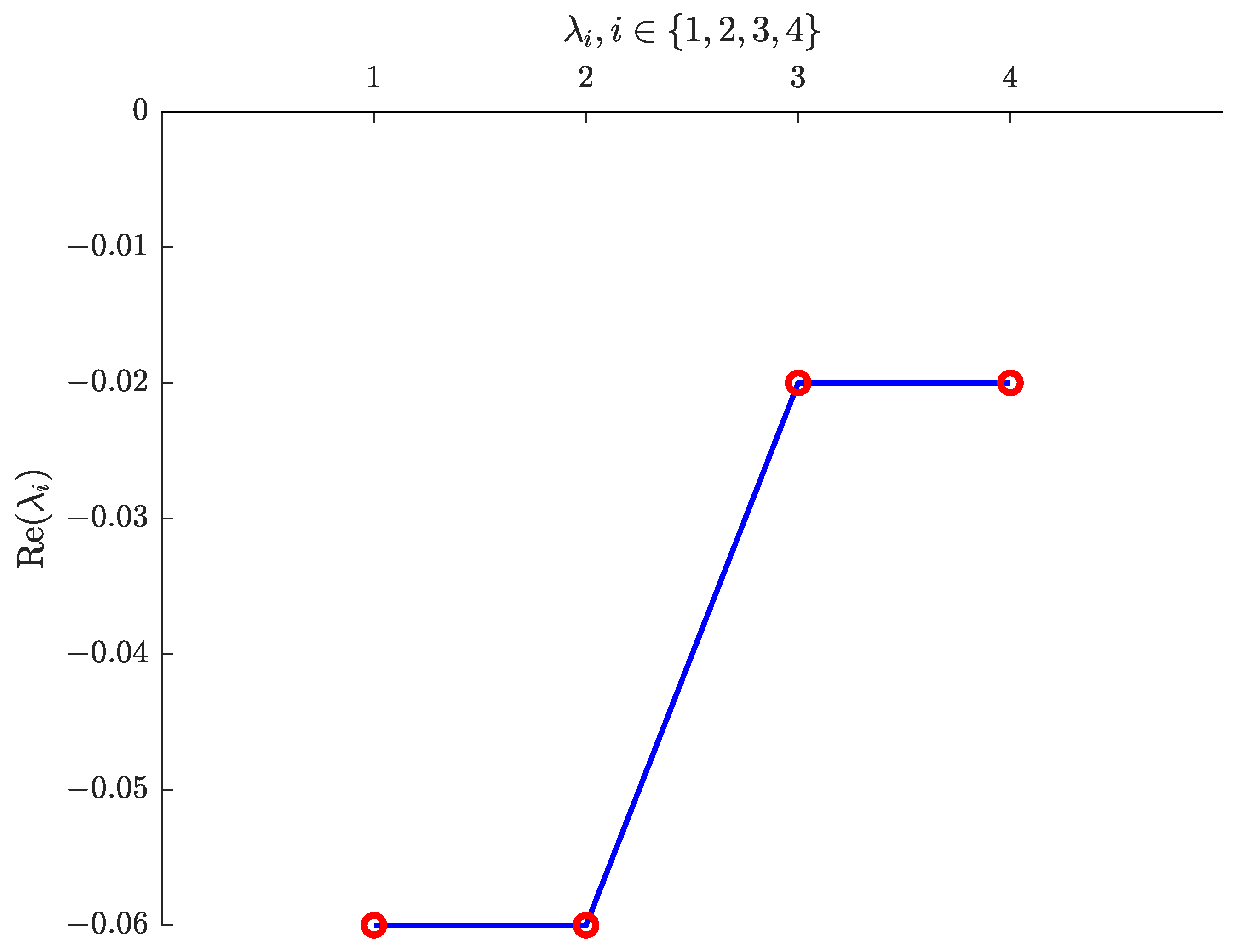
Figure 4.
Negative real parts of the eigenvalues of , for .
Figure 4.
Negative real parts of the eigenvalues of , for .
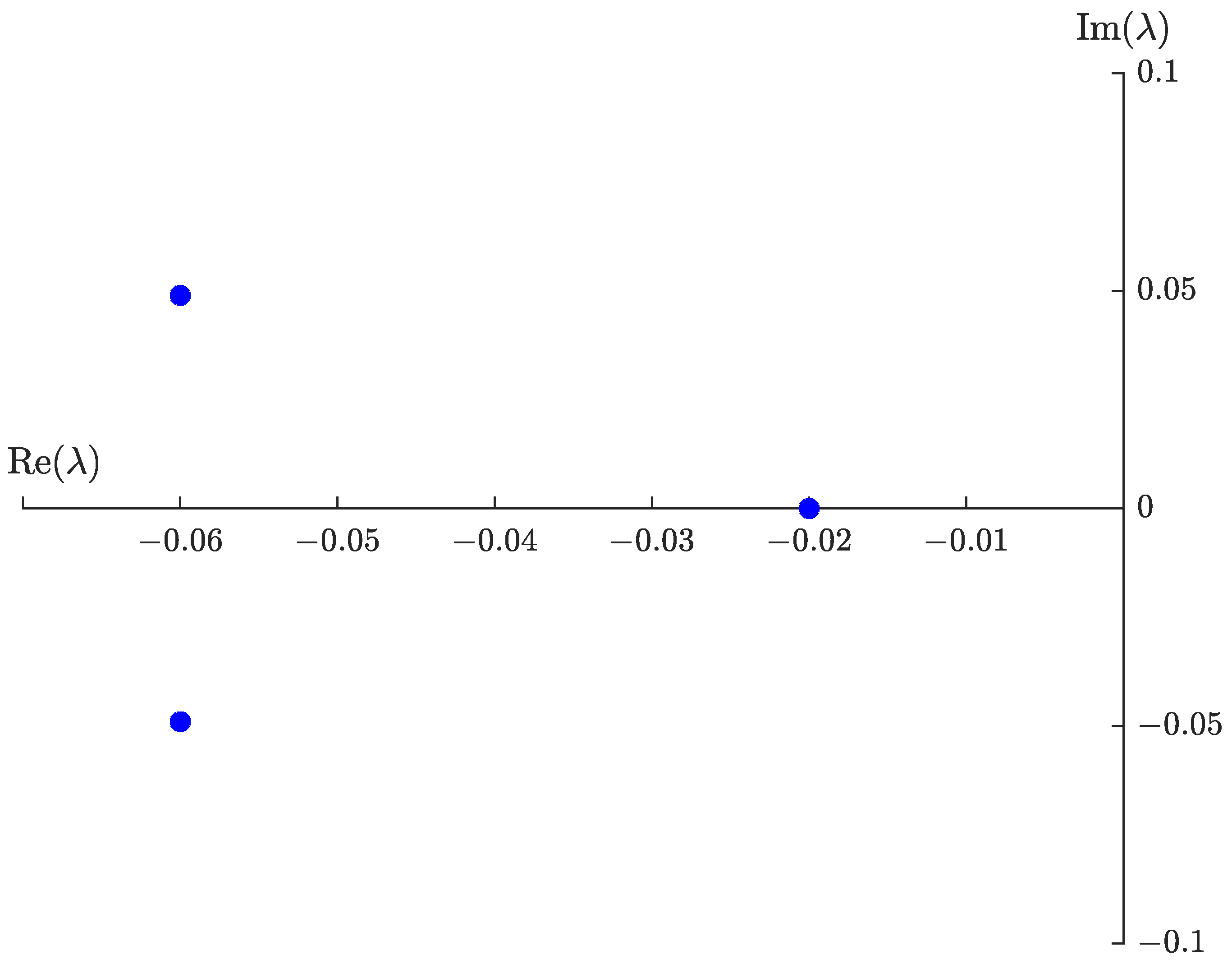
Figure 5.
Real and imaginary parts of the eigenvalues of , for .
Figure 5.
Real and imaginary parts of the eigenvalues of , for .
Figure 6.
Negative real parts of the eigenvalues of , for .
Figure 6.
Negative real parts of the eigenvalues of , for .
Figure 7.
Real and imaginary parts of the eigenvalues of , for .
Figure 7.
Real and imaginary parts of the eigenvalues of , for .
Figure 8.
Negative real parts of the eigenvalues of , for .
Figure 8.
Negative real parts of the eigenvalues of , for .
Figure 9.
Real and Imaginary parts of the eigenvalue of , for .
Figure 9.
Real and Imaginary parts of the eigenvalue of , for .
Figure 10.
3D-phase-portraits of (a) SIV and (b) SIR models.
Figure 10.
3D-phase-portraits of (a) SIV and (b) SIR models.
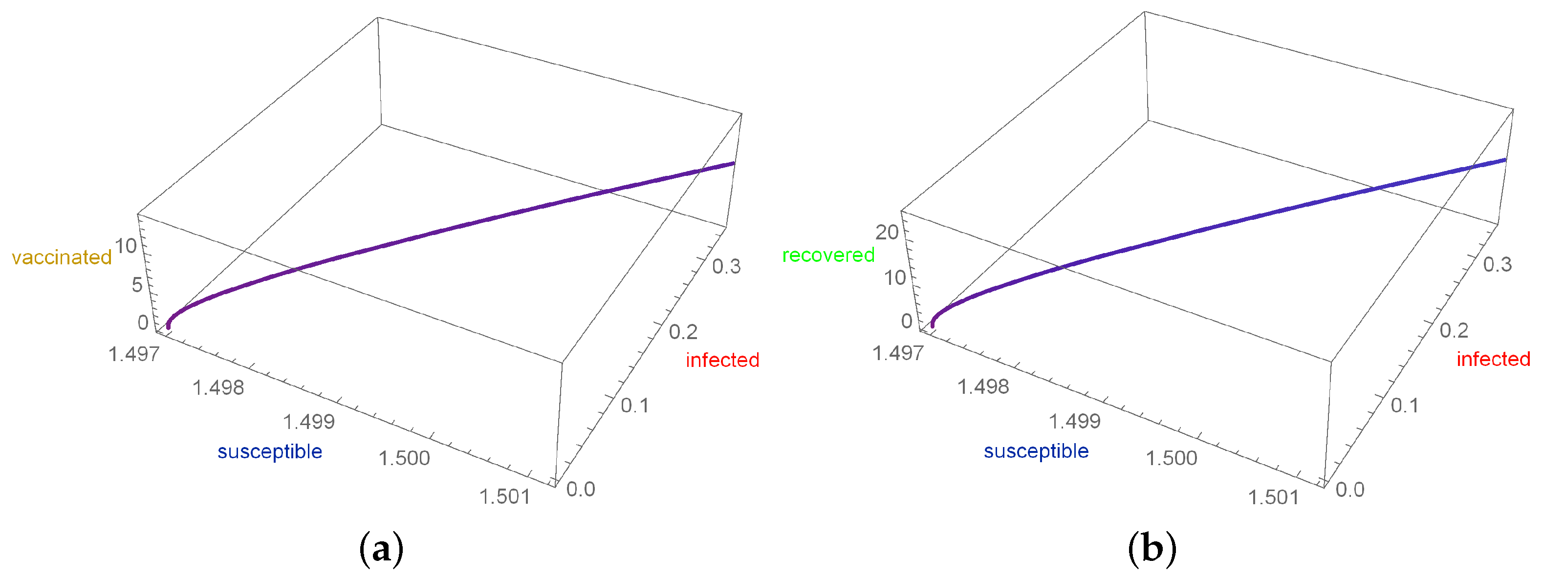
Figure 11.
Parametric plot of the relationship in the SIVR model.
Figure 11.
Parametric plot of the relationship in the SIVR model.
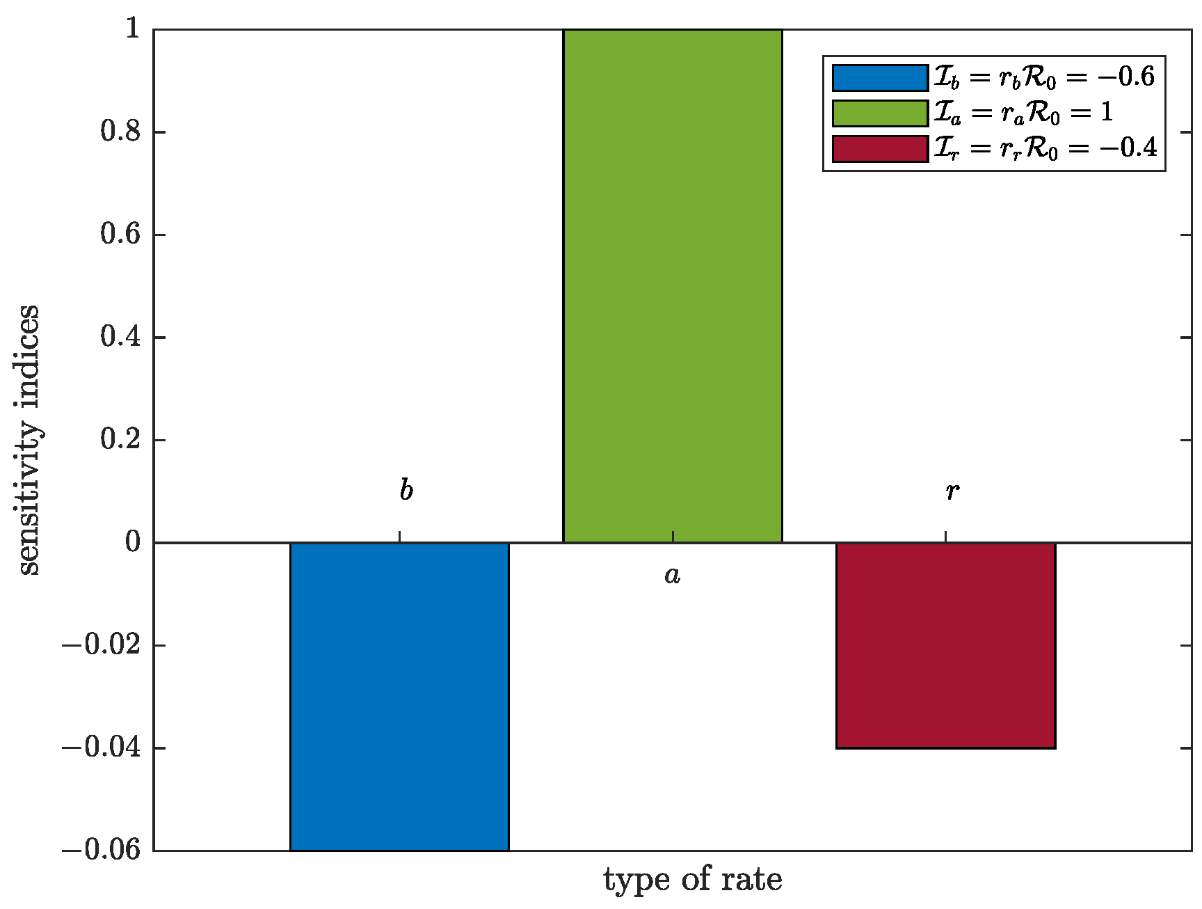
Figure 12.
Bar plot of values of the sensitivity indexes and type of rate.
Figure 12.
Bar plot of values of the sensitivity indexes and type of rate.
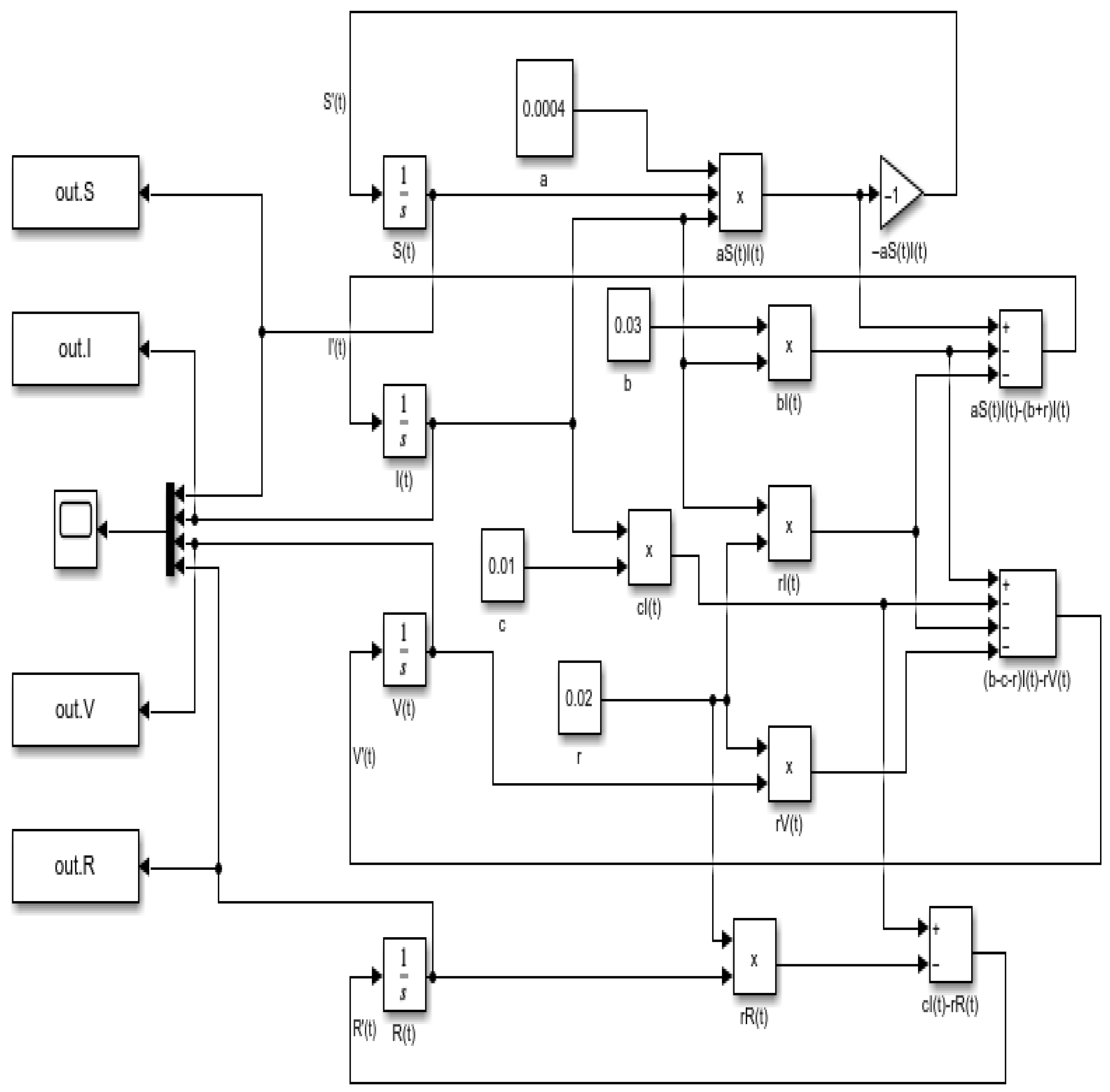
Figure 13.
Block diagram of the SIVR model given in (
1).
Figure 13.
Block diagram of the SIVR model given in (
1).
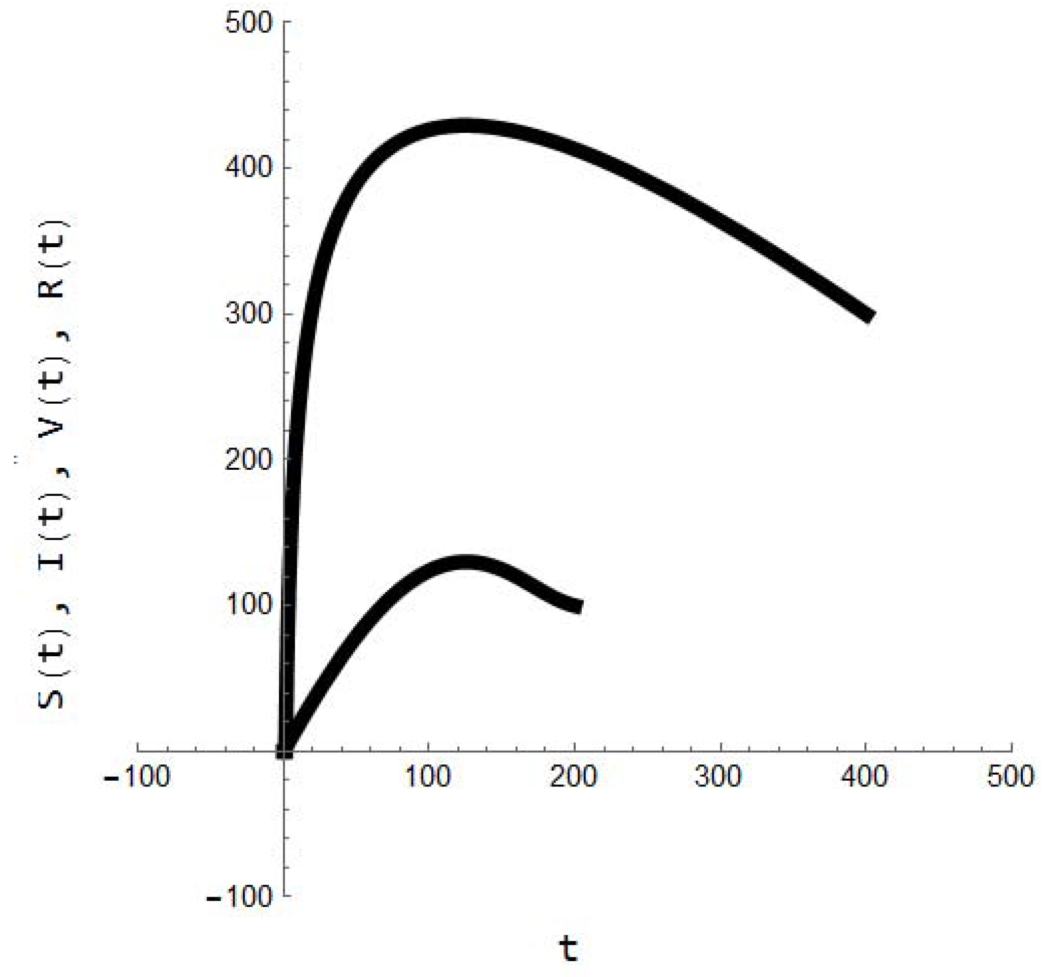
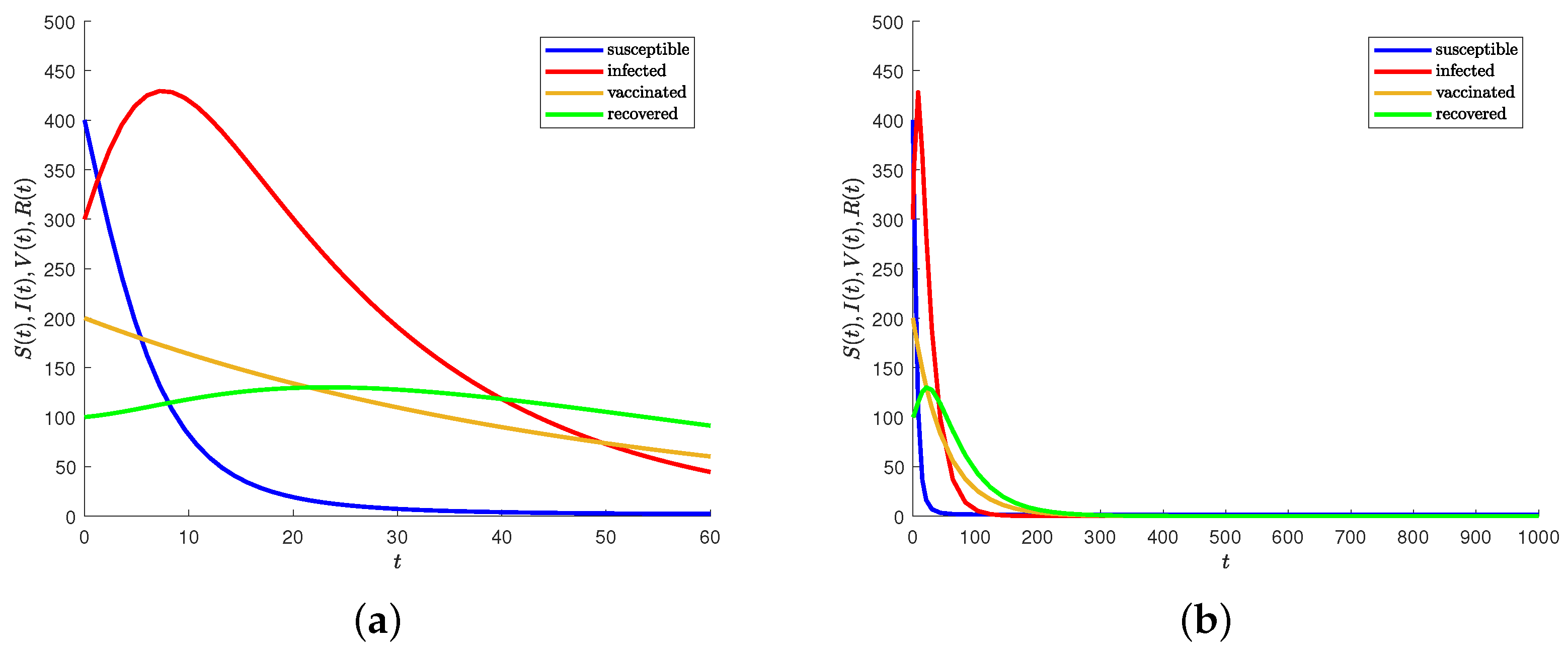
Figure 14.
Plot of the number of susceptible, infected, vaccinated, and recovered people, denoted as , , , and of the SIVR model, respectively, for solutions based on first-order ordinary derivatives over time (a) and (b) in days.
Figure 14.
Plot of the number of susceptible, infected, vaccinated, and recovered people, denoted as , , , and of the SIVR model, respectively, for solutions based on first-order ordinary derivatives over time (a) and (b) in days.
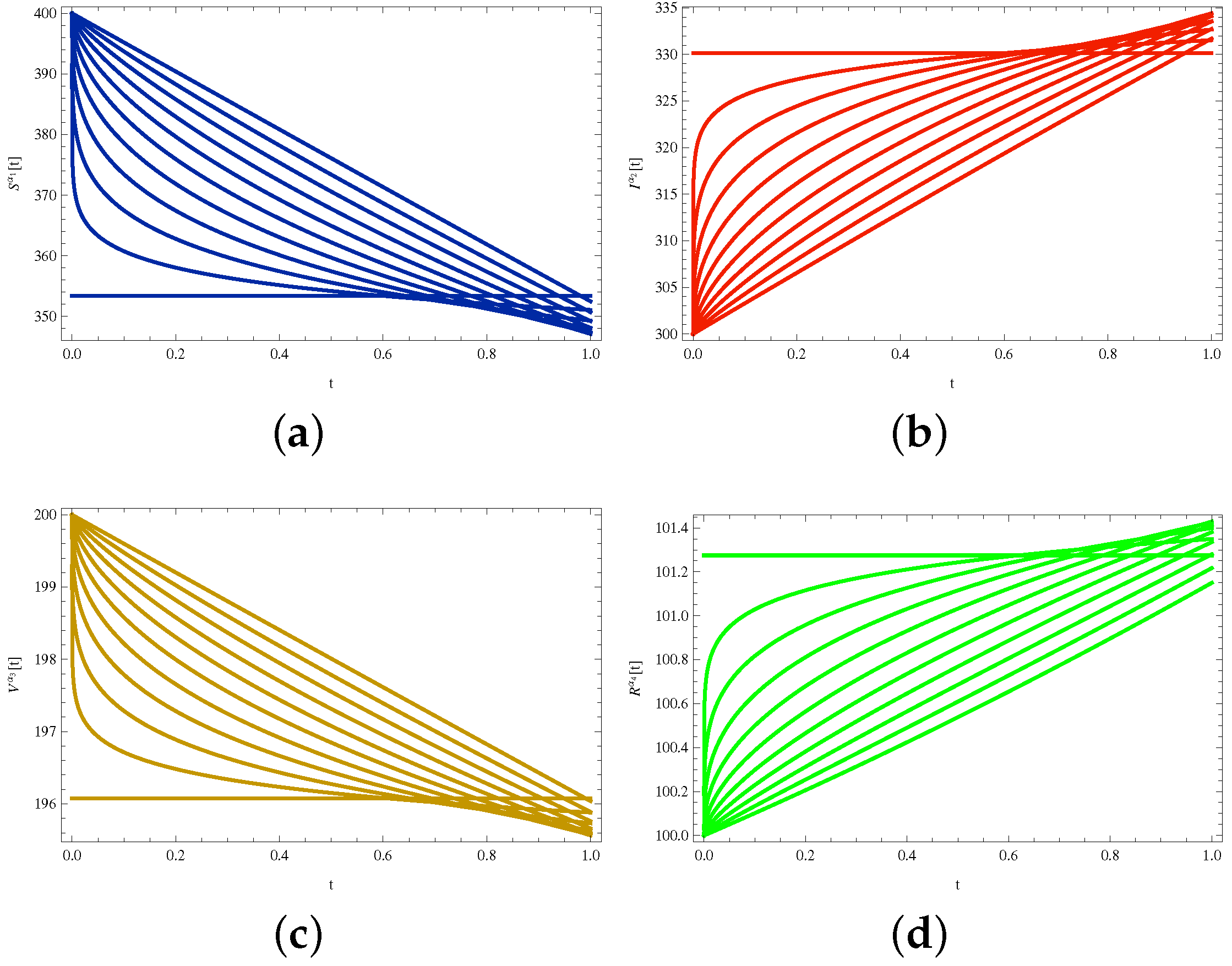
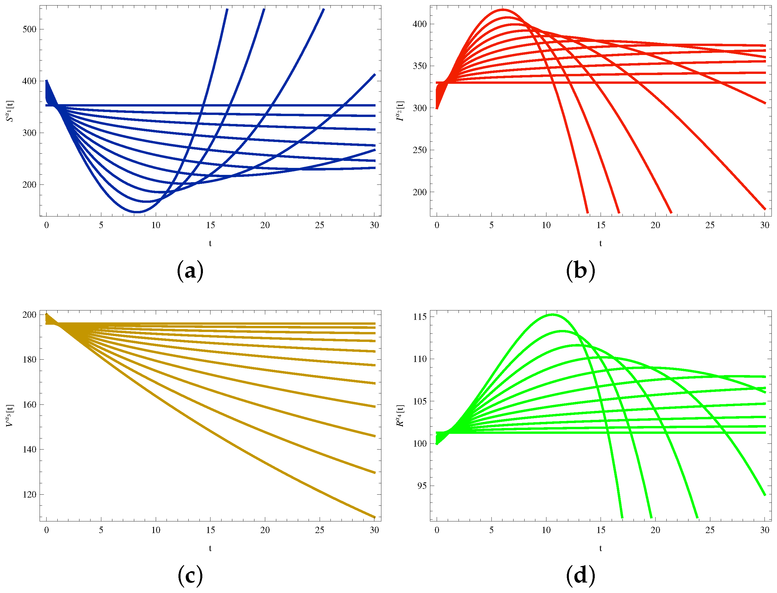
Figure 15.
Plots of the number of (a) susceptible , (b) infected , (c) vaccinated , and (d) recovered cases over time (in days) for 11 solutions each based on the th fractional derivative with for all .
Figure 15.
Plots of the number of (a) susceptible , (b) infected , (c) vaccinated , and (d) recovered cases over time (in days) for 11 solutions each based on the th fractional derivative with for all .
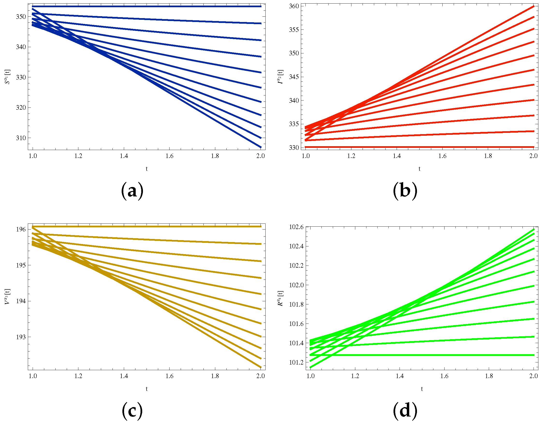
Figure 16.
Plots of the number of (a) susceptible , (b) exposed , (c) infected , and (d) recovered cases over time (in days) for 11 solutions each based on the th fractional derivative with for all .
Figure 16.
Plots of the number of (a) susceptible , (b) exposed , (c) infected , and (d) recovered cases over time (in days) for 11 solutions each based on the th fractional derivative with for all .
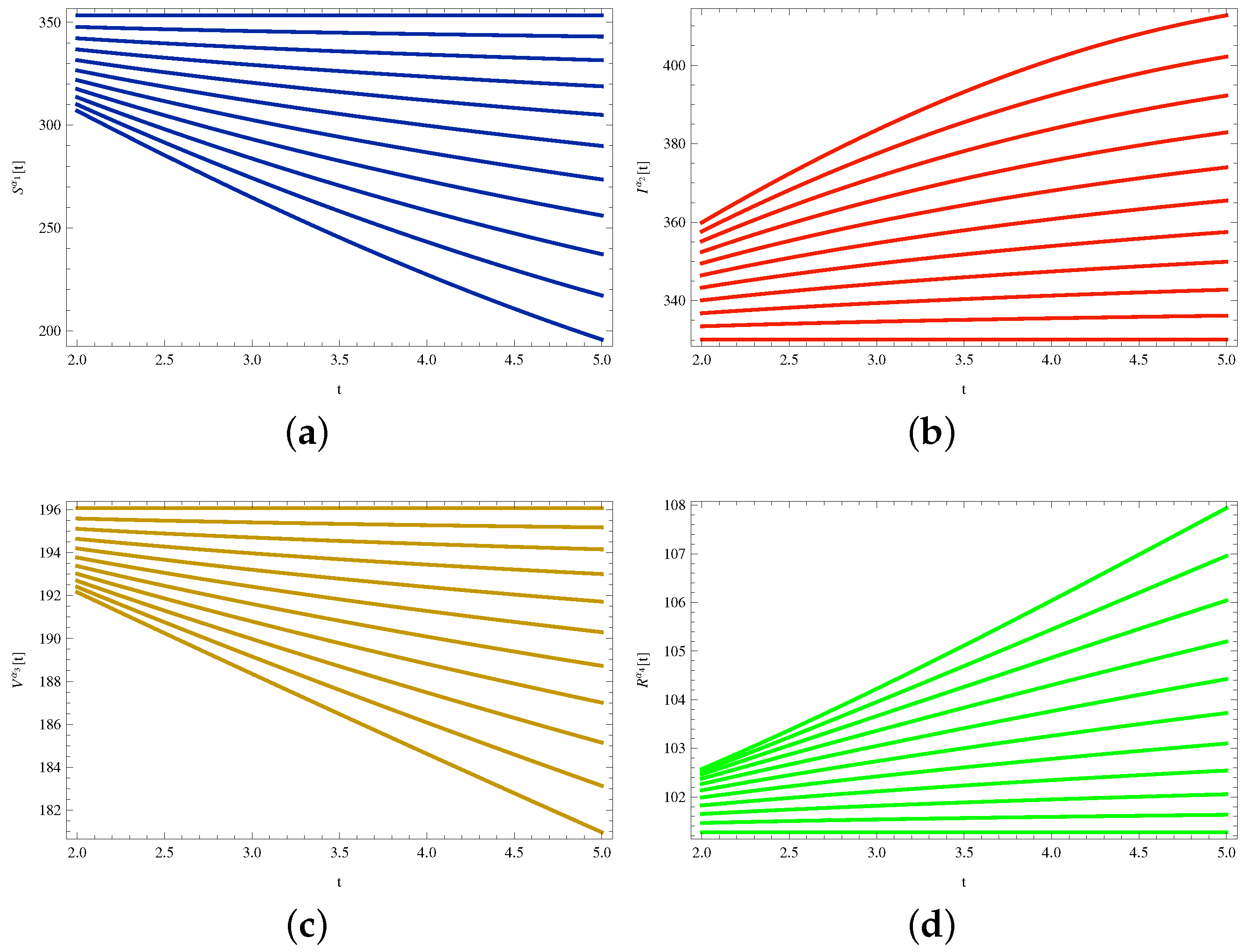
Figure 17.
Plots of the number of (a) susceptible , (b) exposed , (c) infected , and (d) recovered cases over time (in days) for 11 solutions each based on the th fractional derivative with for all .
Figure 17.
Plots of the number of (a) susceptible , (b) exposed , (c) infected , and (d) recovered cases over time (in days) for 11 solutions each based on the th fractional derivative with for all .
Figure 18.
Plots of the number of (a) susceptible , (b) exposed , (c) infected , and (d) recovered cases over time (in days) for 11 solutions each based on the th fractional derivative with for all .
Figure 18.
Plots of the number of (a) susceptible , (b) exposed , (c) infected , and (d) recovered cases over time (in days) for 11 solutions each based on the th fractional derivative with for all .
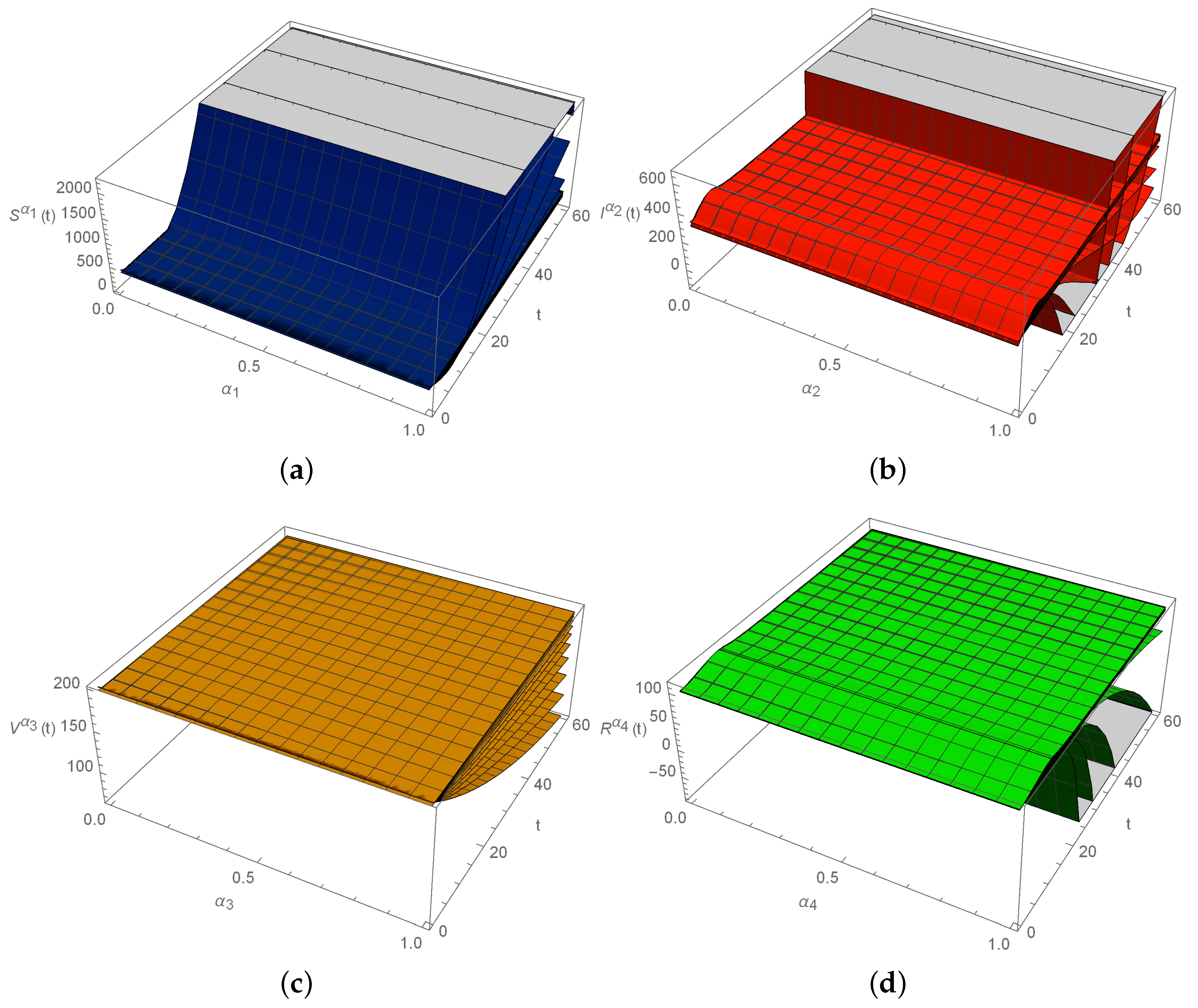
Figure 19.
3D-plots of the number of (a) susceptible , (b) infected , (c) vaccinated , and (d) recovered cases over time (in days) for solutions each based on the th fractional derivative with for all .
Figure 19.
3D-plots of the number of (a) susceptible , (b) infected , (c) vaccinated , and (d) recovered cases over time (in days) for solutions each based on the th fractional derivative with for all .
Table 1.
Notations/symbols employed in the SIVR model and values for
a,
b,
c, and
r as in [
3,
37].
Table 1.
Notations/symbols employed in the SIVR model and values for
a,
b,
c, and
r as in [
3,
37].
| Notations/Symbols | Definition |
|---|
| S | Susceptible population |
| I | Infected population |
| V | Vaccinated population |
| R | Recovered population |
| t | Time instant |
| Initial susceptible population, (fixed) |
| Initial infected population, (fixed) |
| Initial vaccinated population, (fixed) |
| Initial recovered population, (fixed) |
| Threshold point or epidemic critical community size |
| Basic reproduction number |
| a | Rate at which those susceptible become infected, (fixed) |
| b | Rate at which those infected become vaccinated, (fixed) |
| c | Rate at which those infected recover via vaccination, (fixed) |
| r | Rate at which those infected recover naturally, (fixed) |
Table 2.
Simulations with the SIVR model for at for .
Table 2.
Simulations with the SIVR model for at for .
| t | | | | |
|---|
| 0 | 400 | 300 | 200 | 100 |
| 10 | 81.833 | 419.819 | 163.746 | 118.002 |
| 20 | 19.0757 | 300.543 | 134.064 | 129.423 |
| 30 | 7.22778 | 191.081 | 109.762 | 127.787 |
| 40 | 3.93508 | 118.373 | 89.8658 | 118.29 |
| 50 | 2.70459 | 72.7313 | 73.5759 | 105.276 |
| 60 | 2.14891 | 44.5381 | 60.2388 | 91.3616 |
Table 3.
Simulations with the SIVR model for at , for .
Table 3.
Simulations with the SIVR model for at , for .
| t | | | | |
|---|
| 0 | 400 | 300 | 200 | 100 |
| 100 | 1.57405 | 6.19969 | 27.0671 | 45.7696 |
| 200 | 1.4975 | 0.0443779 | 3.66313 | 6.46463 |
| 300 | 1.49697 | 0.000317467 | 0.49575 | 0.876828 |
| 400 | 1.49697 | | 0.0670924 | 0.118679 |
| 500 | 1.49697 | | 0.00907998 | 0.0160616 |
| 600 | 1.49697 | | 0.00122884 | 0.00217371 |
| 700 | 1.49697 | | 0.000166305 | 0.000294179 |
| 800 | 1.49697 | | 0.00002250720 | 0.00003981320 |
| 1000 | 1.49697 | | | |
Table 4.
at and .
Table 4.
at and .
| | |
|---|
| | | | | | | | | | | |
|---|
| 0 | 353.4 | 353.4 | 353.4 | 353.4 | 353.4 | 353.4 | 353.4 | 353.4 | 353.4 | 353.4 | 353.4 |
| 0.1 | 400.0 | 360.8 | 358.0 | 356.4 | 355.2 | 354.2 | 353.4 | 352.7 | 352.1 | 351.6 | 351.1 |
| 0.2 | 400.0 | 367.5 | 362.8 | 359.7 | 357.4 | 355.6 | 354.0 | 352.6 | 351.4 | 350.3 | 349.3 |
| 0.3 | 400.0 | 373.5 | 367.4 | 363.3 | 360.1 | 357.4 | 355.1 | 353.1 | 351.3 | 349.6 | 348.0 |
| 0.4 | 400.0 | 378.6 | 371.9 | 367.0 | 363.1 | 359.7 | 356.7 | 354.1 | 351.7 | 349.4 | 347.3 |
| 0.5 | 400.0 | 382.9 | 375.9 | 370.6 | 366.1 | 362.2 | 358.7 | 355.5 | 352.5 | 349.7 | 347.1 |
| 0.6 | 400.0 | 386.5 | 379.6 | 374.1 | 369.3 | 364.9 | 361.0 | 357.3 | 353.8 | 350.5 | 347.4 |
| 0.7 | 400.0 | 389.5 | 382.9 | 377.4 | 372.4 | 367.8 | 363.4 | 359.3 | 355.4 | 351.7 | 348.1 |
| 0.8 | 400.0 | 391.8 | 385.8 | 380.4 | 375.4 | 370.6 | 366.0 | 361.6 | 357.4 | 353.3 | 349.2 |
| 0.9 | 400.0 | 393.7 | 388.3 | 383.2 | 378.2 | 373.4 | 368.7 | 364.1 | 359.5 | 355.1 | 350.7 |
| 1 | 400.0 | 395.2 | 390.4 | 385.6 | 380.9 | 376.1 | 371.3 | 366.6 | 361.9 | 357.2 | 352.5 |
Table 5.
at and .
Table 5.
at and .
| | |
|---|
| | | | | | | | | | | |
|---|
| 0 | 330.1 | 330.1 | 330.1 | 330.1 | 330.1 | 330.1 | 330.1 | 330.1 | 330.1 | 330.1 | 330.1 |
| 0.1 | 300.0 | 325.7 | 327.3 | 328.3 | 329.1 | 329.7 | 330.1 | 330.6 | 330.9 | 331.2 | 331.5 |
| 0.2 | 300.0 | 321.5 | 324.5 | 326.3 | 327.8 | 328.9 | 329.9 | 330.7 | 331.4 | 332.1 | 332.7 |
| 0.3 | 300.0 | 317.7 | 321.6 | 324.2 | 326.2 | 327.8 | 329.3 | 330.5 | 331.6 | 332.6 | 333.5 |
| 0.4 | 300.0 | 314.4 | 318.8 | 321.9 | 324.4 | 326.5 | 328.4 | 330.0 | 331.5 | 332.9 | 334.1 |
| 0.5 | 300.0 | 311.5 | 316.2 | 319.6 | 322.5 | 325.0 | 327.2 | 329.3 | 331.1 | 332.8 | 334.4 |
| 0.6 | 300.0 | 309.1 | 313.7 | 317.4 | 320.6 | 323.4 | 325.9 | 328.2 | 330.4 | 332.5 | 334.4 |
| 0.7 | 300.0 | 307.2 | 311.6 | 315.3 | 318.6 | 321.6 | 324.4 | 327.0 | 329.5 | 331.9 | 334.1 |
| 0.8 | 300.0 | 305.6 | 309.7 | 313.3 | 316.6 | 319.8 | 322.8 | 325.6 | 328.4 | 331.0 | 333.5 |
| 0.9 | 300.0 | 304.3 | 308.0 | 311.5 | 314.8 | 318.0 | 321.1 | 324.1 | 327.1 | 329.9 | 332.7 |
| 1 | 300.0 | 303.3 | 306.6 | 309.8 | 313.0 | 316.2 | 319.4 | 322.5 | 325.6 | 328.7 | 331.7 |
Table 6.
at and .
Table 6.
at and .
| | |
|---|
| | | | | | | | | | | |
|---|
| 0 | 196.1 | 196.1 | 196.1 | 196.1 | 196.1 | 196.1 | 196.1 | 196.1 | 196.1 | 196.1 | 196.1 |
| 0.1 | 200.0 | 196.7 | 196.5 | 196.3 | 196.2 | 196.2 | 196.1 | 196.0 | 196.0 | 195.9 | 195.9 |
| 0.2 | 200.0 | 197.3 | 196.9 | 196.6 | 196.4 | 196.3 | 196.1 | 196.0 | 195.9 | 195.8 | 195.7 |
| 0.3 | 200.0 | 197.8 | 197.3 | 196.9 | 196.7 | 196.4 | 196.2 | 196.1 | 195.9 | 195.8 | 195.6 |
| 0.4 | 200.0 | 198.2 | 197.7 | 197.2 | 196.9 | 196.6 | 196.4 | 196.2 | 195.9 | 195.8 | 195.6 |
| 0.5 | 200.0 | 198.6 | 198.0 | 197.6 | 197.2 | 196.8 | 196.6 | 196.3 | 196.0 | 195.8 | 195.6 |
| 0.6 | 200.0 | 198.9 | 198.3 | 197.8 | 197.4 | 197.1 | 196.7 | 196.4 | 196.1 | 195.9 | 195.6 |
| 0.7 | 200.0 | 199.1 | 198.6 | 198.1 | 197.7 | 197.3 | 197.0 | 196.6 | 196.3 | 196.0 | 195.7 |
| 0.8 | 200.0 | 199.3 | 198.8 | 198.4 | 197.9 | 197.6 | 197.2 | 196.8 | 196.4 | 196.1 | 195.8 |
| 0.9 | 200.0 | 199.5 | 199.0 | 198.6 | 198.2 | 197.8 | 197.4 | 197.0 | 196.6 | 196.3 | 195.9 |
| 1 | 200.0 | 199.6 | 199.2 | 198.8 | 198.4 | 198.0 | 197.6 | 197.2 | 196.8 | 196.4 | 196.0 |
Table 7.
at and .
Table 7.
at and .
| | |
|---|
| | | | | | | | | | | |
|---|
| 0 | 101.3 | 101.3 | 101.3 | 101.3 | 101.3 | 101.3 | 101.3 | 101.3 | 101.3 | 101.3 | 101.3 |
| 0.1 | 100.0 | 101.0 | 101.1 | 101.2 | 101.2 | 101.2 | 101.3 | 101.3 | 101.3 | 101.3 | 101.4 |
| 0.2 | 100.0 | 100.8 | 101.0 | 101.1 | 101.1 | 101.2 | 101.2 | 101.3 | 101.3 | 101.4 | 101.4 |
| 0.3 | 100.0 | 100.6 | 100.8 | 100.9 | 101.0 | 101.1 | 101.2 | 101.3 | 101.3 | 101.4 | 101.4 |
| 0.4 | 100.0 | 100.5 | 100.7 | 100.8 | 100.9 | 101.0 | 101.1 | 101.2 | 101.3 | 101.4 | 101.4 |
| 0.5 | 100.0 | 100.4 | 100.6 | 100.7 | 100.8 | 100.9 | 101.0 | 101.1 | 101.2 | 101.3 | 101.4 |
| 0.6 | 100.0 | 100.3 | 100.5 | 100.6 | 100.7 | 100.9 | 101.0 | 101.1 | 101.2 | 101.3 | 101.4 |
| 0.7 | 100.0 | 100.2 | 100.4 | 100.5 | 100.6 | 100.8 | 100.9 | 101.0 | 101.1 | 101.2 | 101.3 |
| 0.8 | 100.0 | 100.2 | 100.3 | 100.4 | 100.6 | 100.7 | 100.8 | 100.9 | 101.0 | 101.2 | 101.3 |
| 0.9 | 100.0 | 100.1 | 100.3 | 100.4 | 100.5 | 100.6 | 100.7 | 100.8 | 101.0 | 101.1 | 101.2 |
| 1 | 100.0 | 100.1 | 100.2 | 100.3 | 100.4 | 100.5 | 100.7 | 100.8 | 100.9 | 101.0 | 101.2 |


 ,
, 


