Author Contributions
Conceptualization, M.Ç.K., V.L. and C.M.-B.; data curation, M.Ç.K. and C.M.-B.; formal analysis, M.Ç.K., V.L. and C.M.-B.; investigation, M.Ç.K., V.L. and C.M.-B.; methodology, M.Ç.K., V.L. and C.M.-B.; writing—original draft, M.Ç.K. and C.M.-B.; writing—review and editing, V.L. All authors have read and agreed to the published version of the manuscript.
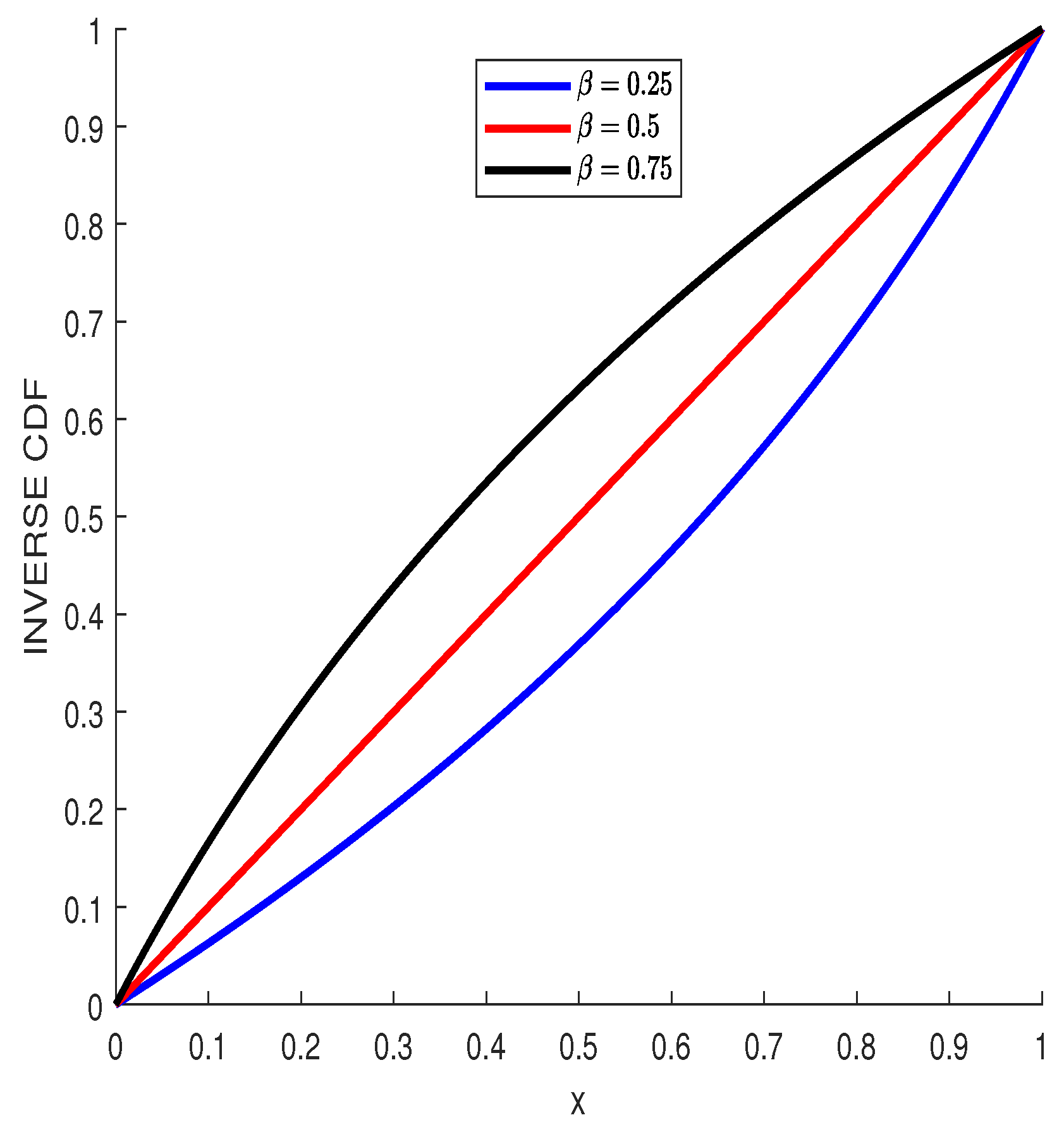
Figure 1.
The CB inverse CDF for the indicated values of .
Figure 1.
The CB inverse CDF for the indicated values of .
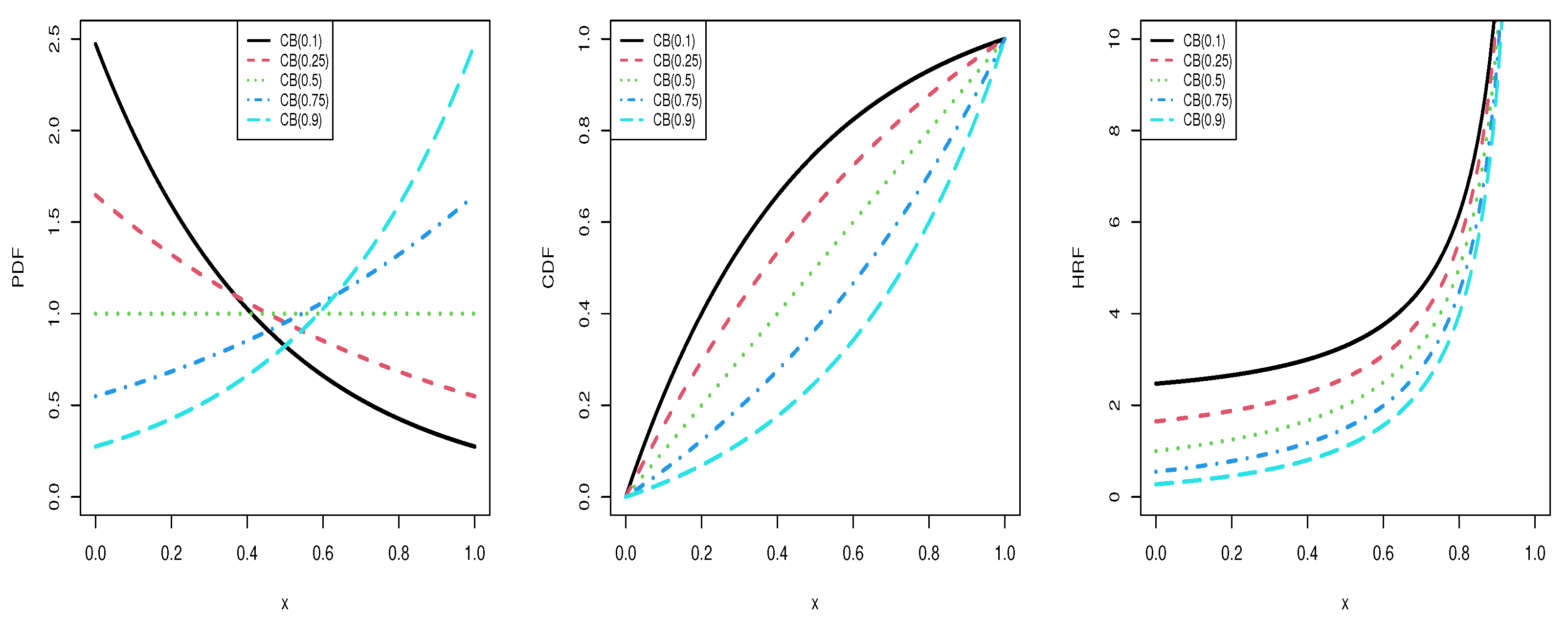
Figure 2.
Plots of the CB PDF (left), CDF (center), and HRF (right) for the listed values of .
Figure 2.
Plots of the CB PDF (left), CDF (center), and HRF (right) for the listed values of .
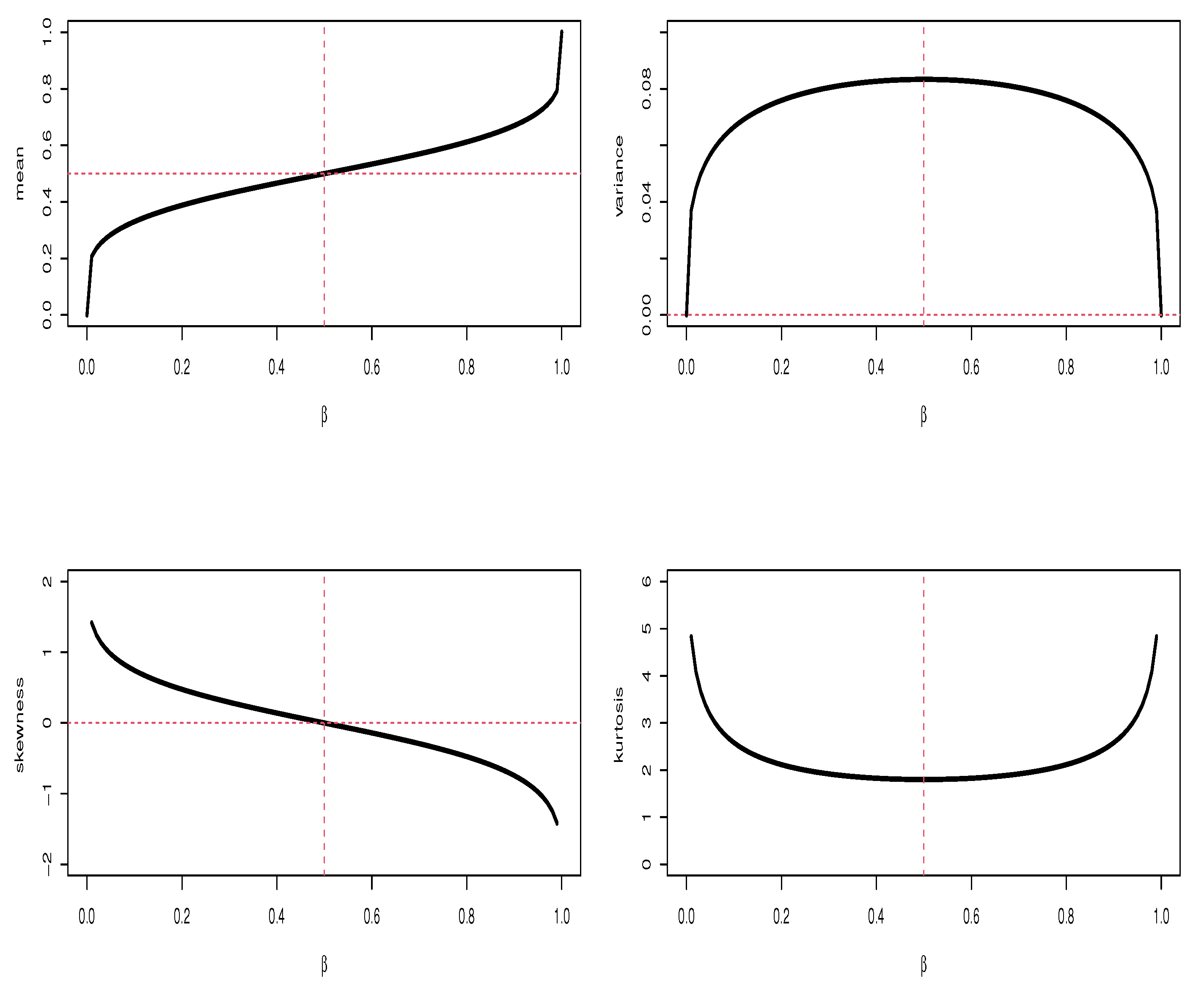
Figure 3.
Plots of the mean, variance, skewness, and kurtosis of the CB distribution for the indicated values of .
Figure 3.
Plots of the mean, variance, skewness, and kurtosis of the CB distribution for the indicated values of .
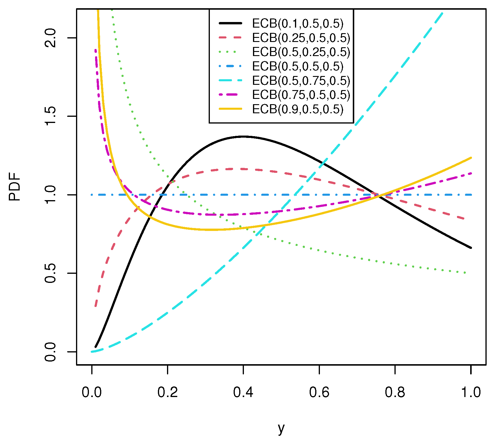
Figure 4.
Plots of the PDF stated in (
14) for the indicated values of parameters.
Figure 4.
Plots of the PDF stated in (
14) for the indicated values of parameters.
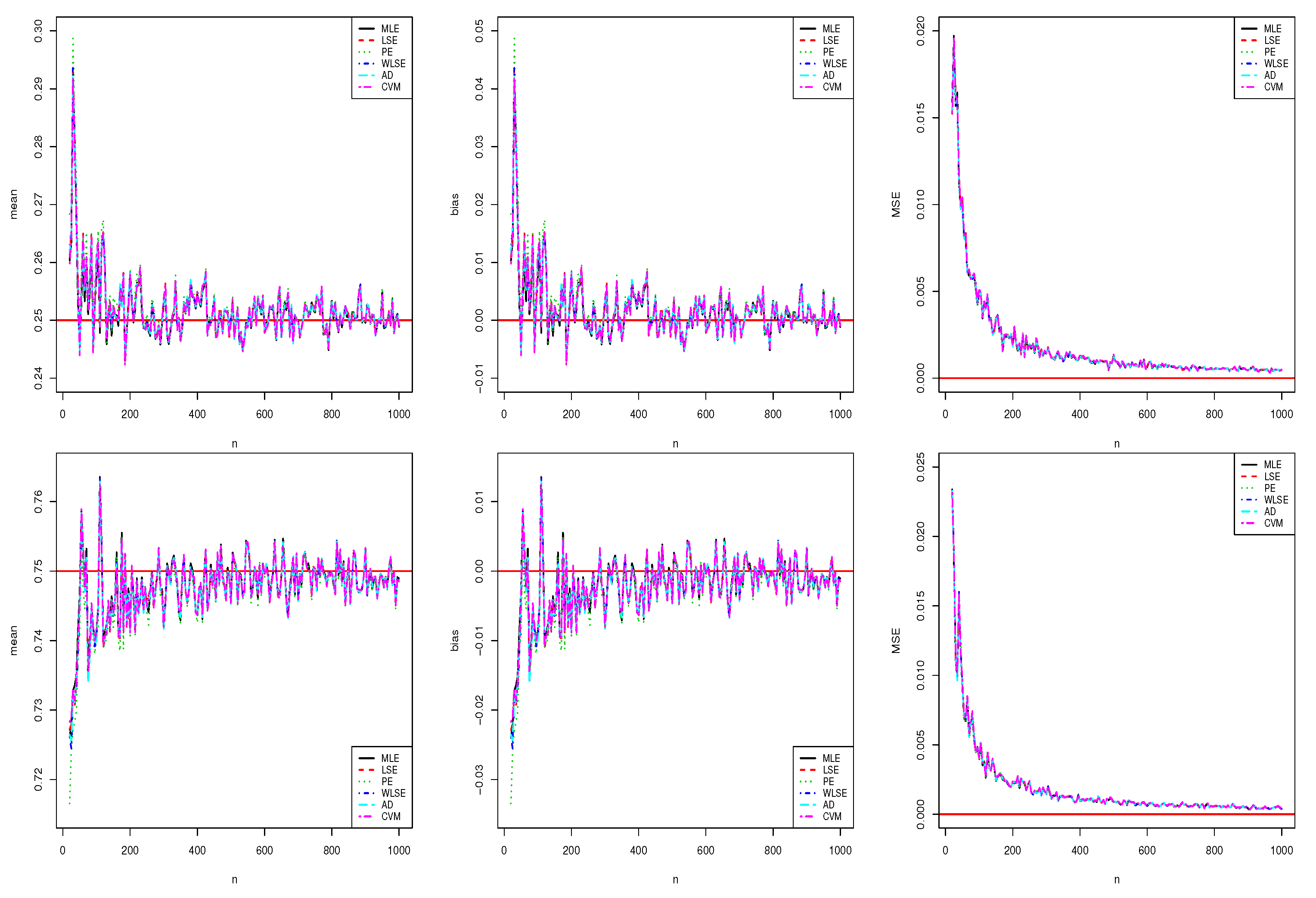
Figure 5.
Plots of simulations for the point estimation with (top) and (bottom).
Figure 5.
Plots of simulations for the point estimation with (top) and (bottom).
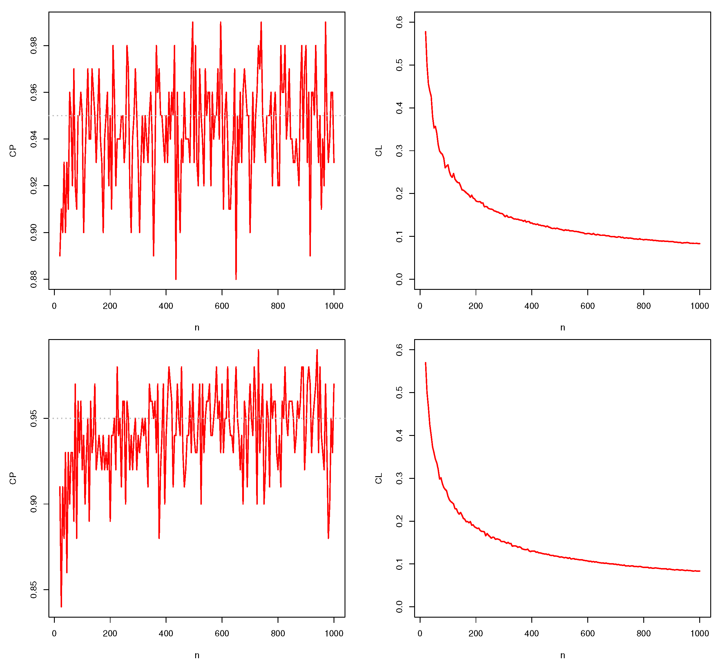
Figure 6.
Plots of simulations for the CPs and CLs with (top) and (bottom).
Figure 6.
Plots of simulations for the CPs and CLs with (top) and (bottom).
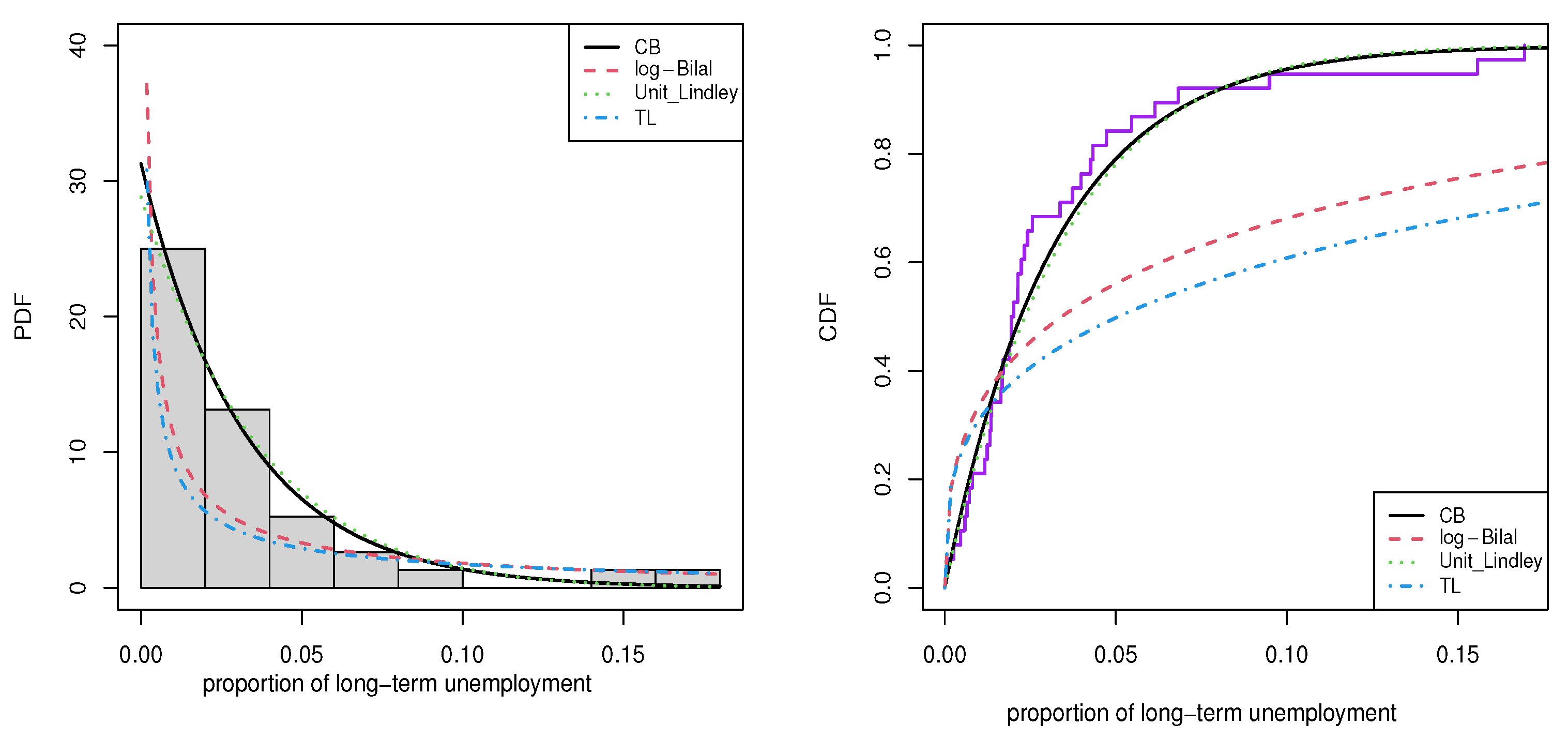
Figure 7.
Plots of fitted PDF (left) and CDF (right) for the unemployment data.
Figure 7.
Plots of fitted PDF (left) and CDF (right) for the unemployment data.
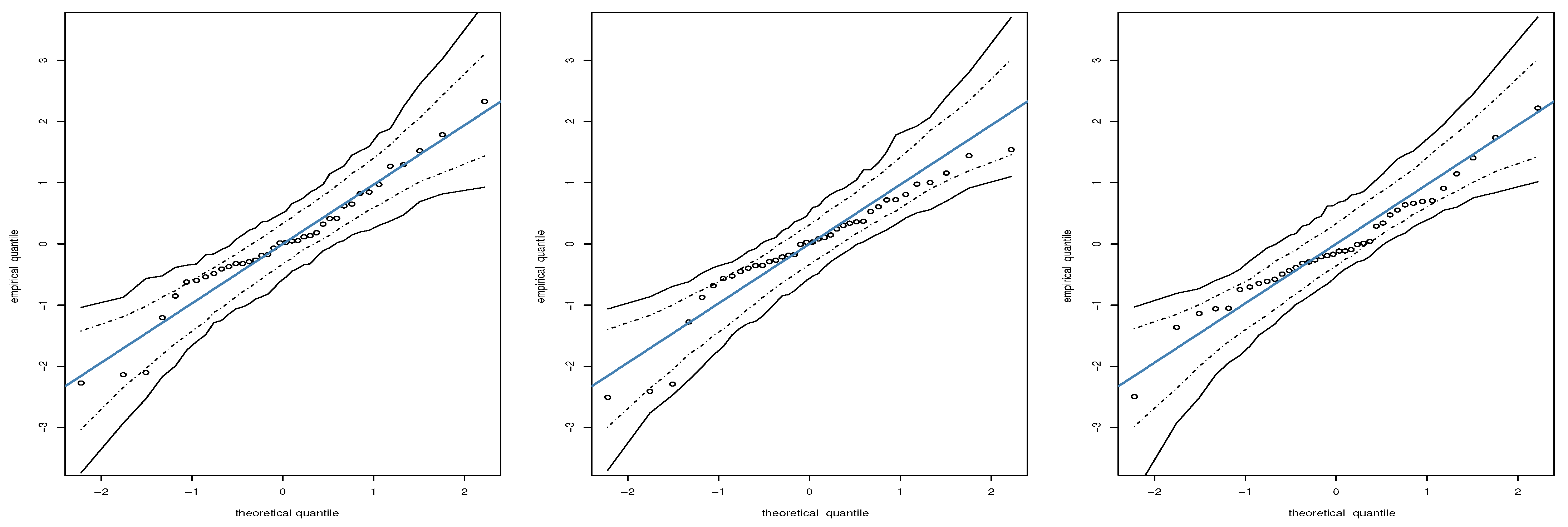
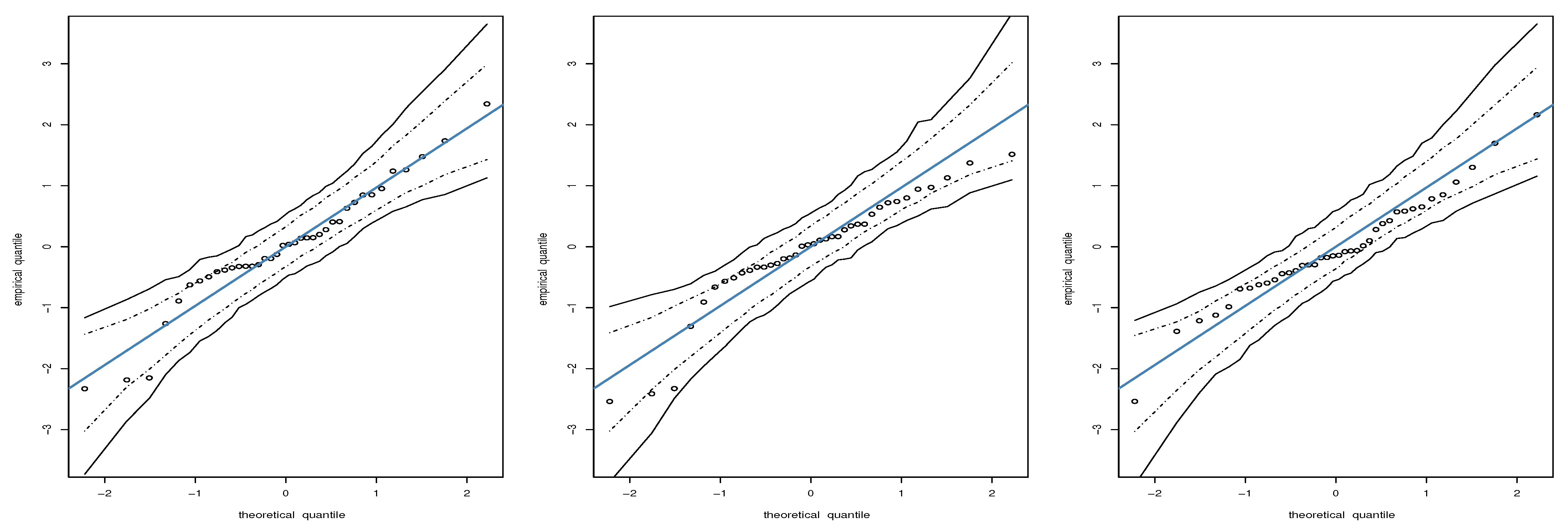
Figure 8.
QQ plots of the RQ residual for KW (left), LEEG (center), and ECB (right) models based on quantile level with educational data, where circles indicate the observed data.
Figure 8.
QQ plots of the RQ residual for KW (left), LEEG (center), and ECB (right) models based on quantile level with educational data, where circles indicate the observed data.
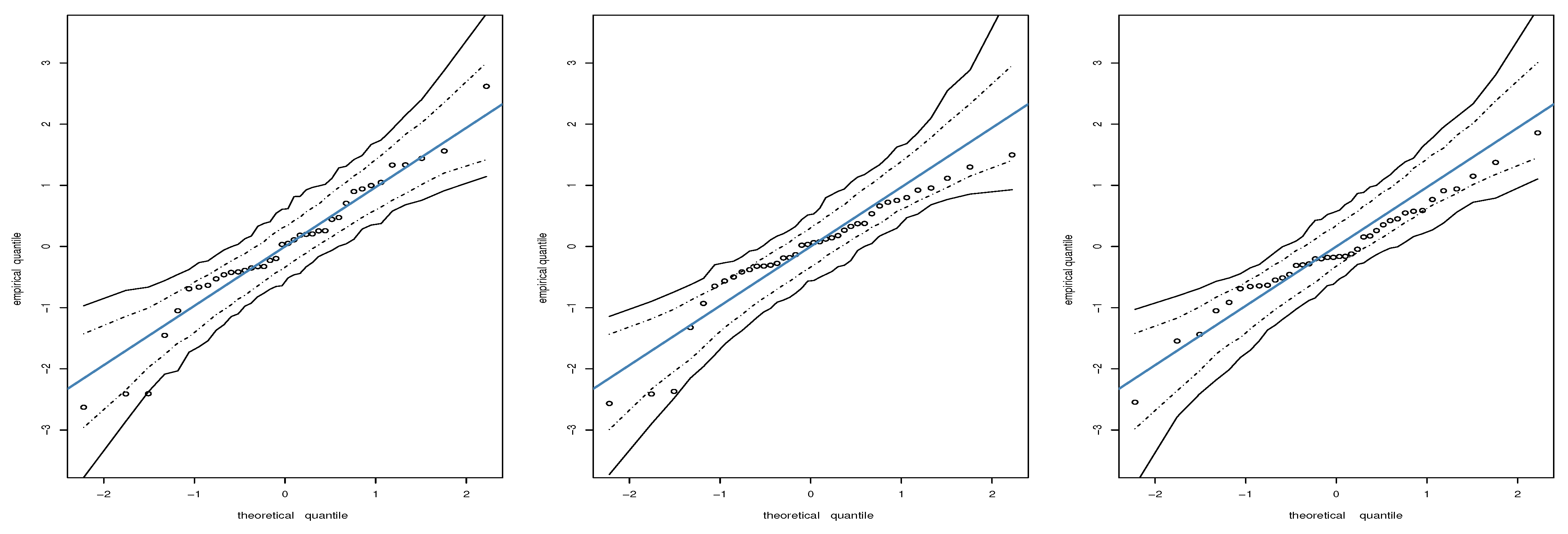
Figure 9.
QQ plots of the RQ residual for KW (left), LEEG (center), and ECB (right) models based on quantile level with educational data, where circles indicate the observed data.
Figure 9.
QQ plots of the RQ residual for KW (left), LEEG (center), and ECB (right) models based on quantile level with educational data, where circles indicate the observed data.
Figure 10.
QQ plots of the RQ residual for KW (left), LEEG (center), and ECB (right) models based on quantile level with educational data, where circles indicate the observed data.
Figure 10.
QQ plots of the RQ residual for KW (left), LEEG (center), and ECB (right) models based on quantile level with educational data, where circles indicate the observed data.
Table 1.
Simulation results with .
Table 1.
Simulation results with .
| n | Runtime (in Seconds) | | |
|---|
| 25 | | | |
| 50 | | | |
| 100 | | | |
| 200 | | | |
| 500 | | | |
| 1000 | | | |
Table 2.
Simulation results with .
Table 2.
Simulation results with .
| n | Runtime (in Seconds) | | |
|---|
| 25 | | | |
| 50 | | | |
| 100 | | | |
| 200 | | | |
| 500 | | | |
| 1000 | | | |
Table 3.
Empirical bias, MSE, CP, and CL for the ECB QR model with and for the indicated n and parameter with simulated data.
Table 3.
Empirical bias, MSE, CP, and CL for the ECB QR model with and for the indicated n and parameter with simulated data.
| n | Bias() | Bias() | Bias() | MSE() | MSE() | MSE() | CL() | CL() | CL() | CP() | CP() | CP() |
|---|
| 25 | | | | | | | | | | | | |
| 50 | | | | | | | | | | | | |
| 100 | | | | | | | | | | | | |
| 200 | | | | | | | | | | | | |
| 500 | | | | | | | | | | | | |
| 1000 | | | | | | | | | | | | |
Table 4.
Empirical bias, MSE, CP, and CL for the ECB QR model with and for the indicated n and parameter with simulated data.
Table 4.
Empirical bias, MSE, CP, and CL for the ECB QR model with and for the indicated n and parameter with simulated data.
| n | Bias() | Bias() | Bias() | MSE() | MSE() | MSE() | CL() | CL() | CL() | CP() | CP() | CP() |
|---|
| 25 | | | | | | | | | | | | |
| 50 | | | | | | | | | | | | |
| 100 | | | | | | | | | | | | |
| 200 | | | | | | | | | | | | |
| 500 | | | | | | | | | | | | |
| 1000 | | | | | | | | | | | | |
Table 5.
Empirical bias, MSE, CP, and CL for the ECB QR model with and for the indicated n and parameter with simulated data.
Table 5.
Empirical bias, MSE, CP, and CL for the ECB QR model with and for the indicated n and parameter with simulated data.
| n | Bias() | Bias() | MSE() | MSE() | CL() | CL() | CP() | CP() |
|---|
| 25 | | | | | | | | |
| 50 | | | | | | | | |
| 100 | | | | | | | | |
| 200 | | | | | | | | |
| 500 | | | | | | | | |
| 1000 | | | | | | | | |
Table 6.
Empirical bias, MSE, CP, and CL for the ECB QR model with and for the indicated n and parameter with simulated data.
Table 6.
Empirical bias, MSE, CP, and CL for the ECB QR model with and for the indicated n and parameter with simulated data.
| n | Bias() | Bias() | MSE() | MSE() | CL() | CL() | CP() | CP() |
|---|
| 25 | | | | | | | | |
| 50 | | | | | | | | |
| 100 | | | | | | | | |
| 200 | | | | | | | | |
| 500 | | | | | | | | |
| 1000 | | | | | | | | |
Table 7.
Empirical bias, MSE, CP, and CL for the ECB QR model with and for the indicated n and parameter with simulated data.
Table 7.
Empirical bias, MSE, CP, and CL for the ECB QR model with and for the indicated n and parameter with simulated data.
| n | Bias() | Bias() | Bias() | MSE() | MSE() | MSE() | CL() | CL() | CL() | CP() | CP() | CP() |
|---|
| 25 | | | | | | | | | | | | |
| 50 | | | | | | | | | | | | |
| 100 | | | | | | | | | | | | |
| 200 | | - | | | | | | | | | | |
| 500 | | - | | | | | | | | | | |
| 1000 | | - | | | | | | | | | | |
Table 8.
Empirical bias, MSE, CP, and CL for the ECB QR model with and for the indicated n and parameter with simulated data.
Table 8.
Empirical bias, MSE, CP, and CL for the ECB QR model with and for the indicated n and parameter with simulated data.
| n | Bias() | Bias() | Bias() | MSE() | MSE() | MSE() | CL() | CL() | CL() | CP() | CP() | CP() |
|---|
| 25 | | | | | | | | | | | | |
| 50 | | | | | | | | | | | | |
| 100 | | | | | | | | | | | | |
| 200 | | | | | | | | | | | | |
| 500 | | | | | | | | | | | | |
| 1000 | | | | | | | | | | | | |
Table 9.
ML estimate and standard errors, in parentheses, as well as and p-value of the goodness-of-fit test, in brackets, with unemployment data.
Table 9.
ML estimate and standard errors, in parentheses, as well as and p-value of the goodness-of-fit test, in brackets, with unemployment data.
| Distribution | | | AIC | BIC | AD | CM | KS |
|---|
| CB | | | | | | | |
| Log-Bilal | | | | | | | |
| TL | | | | | | | |
| Unit-Lindley | | | | | | | |
Table 10.
Results of fitted regressions with quantile and model selection criteria for educational data.
Table 10.
Results of fitted regressions with quantile and model selection criteria for educational data.
| Parameter | ECB | KW | LEEG |
|---|
| | Estimate | SE | p-Value | Estimate | SE | p-Value | Estimate | SE | p-Value |
|---|
| 1.9160 | 0.3172 | <0.0001 | 1.3473 | 0.1730 | <0.0001 | 1.4199 | 0.1599 | <0.0001 |
| −0.0914 | 0.0241 | <0.0001 | −0.0511 | 0.0130 | <0.0001 | −0.05588 | 0.0118 | <0.0001 |
| 11.1800 | 2.3920 | <0.0001 | 2.0563 | 1.1999 | 0.0866 | 2.3612 | 1.3068 | 0.078 |
| −21.2000 | 6.1390 | <0.001 | −7.1977 | 1.1596 | <0.0001 | −8.1841 | 1.7661 | <0.0001 |
| 0.00058 | 0.0009 | 0.5367 | 7.0769 | 1.2104 | <0.0001 | 9.1738 | 1.9582 | <0.0001 |
| 35.5794 | 33.5838 | 32.3569 |
| AIC | −61.1587 | −57.1676 | −54.7139 |
| BIC | −52.9708 | −48.9797 | −46.5259 |
Table 11.
Results of fitted regressions with quantile and model selection criteria for educational data.
Table 11.
Results of fitted regressions with quantile and model selection criteria for educational data.
| Parameter | ECB | KW | LEEG |
|---|
| | Estimate | SE | p-Value | Estimate | SE | p-Value | Estimate | SE | p-Value |
|---|
| 2.3830 | 1.7410 | <0.0001 | 1.9595 | 0.1795 | <0.0001 | 1.9907 | 0.1903 | <0.0001 |
| −0.0942 | 0.0207 | <0.0001 | −0.0639 | 0.0135 | <0.0001 | −0.0671 | 0.0134 | <0.0001 |
| 10.9300 | 2.2890 | <0.0001 | 2.3783 | 1.2035 | 0.0481 | 2.8145 | 1.4914 | 0.0591 |
| −21.0700 | 1.8860 | <0.0001 | −8.9696 | 1.3384 | <0.0001 | −9.8119 | 2.0626 | <0.0001 |
| 0.00097 | 0.0015 | 0.513 | 7.2166 | 1.2191 | <0.0001 | 9.1091 | 1.9682 | <0.0001 |
| 34.6717 | 33.8642 | 32.2079 |
| AIC | −59.3433 | −57.7286 | −54.4158 |
| BIC | −51.1553 | −49.5406 | −46.2279 |
Table 12.
Results of fitted regressions with quantile and model selection criteria for educational data.
Table 12.
Results of fitted regressions with quantile and model selection criteria for educational data.
| Parameters | ECB | KW | LEEG |
|---|
| | Estimate | SE | p-Value | Estimate | SE | p-Value | Estimate | SE | p-Value |
|---|
| 3.0897 | 0.2262 | <0.0001 | 2.5204 | 0.2044 | <0.0001 | 2.7506 | 0.2707 | <0.0001 |
| −0.0978 | 0.0229 | <0.0001 | −0.0772 | 0.0133 | <0.0001 | −0.0834 | 0.0157 | <0.0001 |
| 9.7876 | 1.8659 | <0.0001 | 2.7295 | 1.5489 | 0.0708 | 3.5070 | 1.8068 | 0.0523 |
| −19.9055 | 1.4959 | <0.0001 | −10.0828 | 1.6659 | <0.0001 | −12.1760 | 2.6050 | <0.0001 |
| 0.0022 | 0.0029 | 0.4530 | 8.2613 | 1.3396 | <0.0001 | 9.0614 | 2.0043 | <0.0001 |
| 33.8923 | 33.6323 | 32.0757 |
| AIC | −57.7847 | −57.2647 | −54.1515 |
| BIC | −49.5967 | −49.0768 | −45.9635 |


