Electromagnetic Scattering from Fractional Brownian Motion Surfaces via the Small Slope Approximation

Abstract

Marine and terrestrial natural surfaces exhibit statistical scale invariance properties that are well modelled by fractional Brownian motion (fBm), two-dimensional random processes. Accordingly, for microwave remote sensing applications it is useful to evaluate the normalized radar cross section (NRCS) of fBm surfaces. This task has been accomplished in the past by using either the Kirchhoff approximation (KA) or the small perturbation method (SPM). However, KA and SPM have rather limited ranges of application in terms of surface roughness and incidence angle: a wider range of application is achieved by the small slope approximation (SSA), more recently developed, but the latter has not been applied yet to fBm surfaces. In this paper, the first-order SSA (SSA-1) is applied to the evaluation of scattering from fBm surfaces obtaining an analytical formulation of their NRCS. It is then shown that the obtained SSA-1 expression reduces to the KA and SPM ones at near-specular and far-from-specular scattering directions, respectively. Finally, the results of the proposed method are compared to experimental data available in the literature.

1. Introduction

In microwave remote sensing applications, establishing a relationship between the intensity of the electromagnetic field scattered by a soil or sea surface and the geometric and electromagnetic parameters characterizing the scattering surface is of paramount importance [1,2,3]. To this aim, the surface roughness is usually modeled as a two-dimensional (2D) zero-mean random process, and it is often assumed that the random process is statistically stationary, so that it is synthetically described in terms of its root mean square (rms) height σ and correlation length L or sometimes in terms of its rms slope σ_s [1,2,3]. However, experimental data show that, for soil surfaces, measured values of σ and L increase with the length of the considered height profile [4,5,6], and it is well known that the measured rms slope of a sea surface increases with the maximum spatial frequency that is considered to estimate it [6,7,8]. Accordingly, σ, L and rms slope are not well suited to characterize the roughness of natural surfaces. This is related to the fact that soil and sea surfaces exhibit power-law spectra over a wide range of spatial frequencies and show scale invariance statistical properties over a wide range of scales. Both features can be accounted for by modelling the roughness of natural surfaces as fractional Brownian motion (fBm), two-dimensional processes [4,5]. Such fractal processes are not statistically stationary so that the application of usual methods for the evaluation of scattering from randomly rough surfaces requires some effort. Actually, while fractals have been widely used in the design of antennas and metamaterials [9,10,11,12,13,14], and, more recently, in some cases also of metasurfaces and reflecting intelligent surfaces (RIS) [15], their use in electromagnetic scattering from rough surfaces is not so widespread. Currently, some analytical evaluations of scattering from fBm surfaces are available, most of which employing the Kirchhoff approximation (KA) [16,17,18,19], and a few others the small perturbation method (SPM) [20], possibly within a two-scale model (TSM) [8,21]. KA and SPM, which were developed in the middle of last century [22,23], have rather limited ranges of application in terms of surface roughness and incidence angle. A wider range of application is achieved by the small slope approximation (SSA) that has been developed more recently [24,25]. In this paper, we apply the first-order SSA (SSA-1) to the evaluation of the normalized radar cross section (NRCS) of fBm surfaces and we show that the obtained SSA-1 NRCS reduces to the KA and SPM ones in their respective ranges of validity. In order to do that, we also have to reformulate the ranges of validity in terms of fBm parameters. This leads to defining an effective surface slope variance that depends on wavelength and on viewing geometry. Finally, we show that the results of the proposed method compare favorably with experimental data available in the literature.

2. Theory

2.1. fBm Surface

Height deviations, z(x,y), of a rough surface with respect to its mean plane are usually modelled by a zero-mean Gaussian random process. If the process is statistically stationary, it is fully characterized by its autocorrelation function ${\sigma }^{2}C\left(\mathsf{\Delta }x,\mathsf{\Delta }y\right)$, i.e., the mean value of z(x + Δx,y + Δy)z(x,y), or equivalently, by its power spectral density (PSD, or simply spectrum). In fact, in this case the spectrum is the Fourier transform of the autocorrelation function.

A 2D fBm is a random process z(x,y) whose increments z(x + Δx,y + Δy) − z(x,y) over a fixed horizontal distance $\rho =\sqrt{\mathsf{\Delta }{x}^2+\mathsf{\Delta }{y}^2}$ are zero-mean Gaussian random variables with variance

$$Q_{fBm}\left(\rho \right)=s^2{\rho }^{2H}$$

(1)

where s is a parameter measured in m^1−H, numerically coincident with the standard deviation of increments over 1 m distance, and H is the Hurst coefficient, with 0 < H < 1 [4,5]. Realizations of a 2D fBm process are fractal surfaces with fractal dimension D = 3 − H.

The fBm process is not statistically stationary, so that its spectrum cannot be expressed as the Fourier transform of the autocorrelation function. However, it is a stationary-increment process, so that its spectrum can be related to the function (1), called structure function. It can be shown that the PSD of an fBm follows a power law [4,5,19]:

$$S_{fBm}\left({\kappa }_x,{\kappa }_y\right)=S_0{\kappa }^{-\alpha }$$

(2)

where ${\kappa }_x \mathrm{and} {\kappa }_y$ are the x and y components of the surface wavenumber vector κ, $\kappa =\sqrt{{\kappa }_x^2+{\kappa }_y^2}$ is its modulus,

$$\alpha =2+2H, S_0=\pi H{2}^{1+2H}\frac{\mathsf{\Gamma }\left(1+H\right)}{\mathsf{\Gamma }\left(1-H\right)}{s}^2$$

(3)

and $\mathsf{\Gamma }(·)$ is the gamma function.

The variance of an fBm process is infinite; however, the measured variance ${\sigma }^2$ of the height of a patch of fBm surface of linear size $l$ is finite and increases with $l$:

$${\sigma }^2\left(l\right)=\frac{1}{2}{s}^2{l}^{2H}$$

(4)

Similarly, the variance of slopes of an fBm process are infinite (actually, realizations of an fBm process are not differentiable); however, the variance of slopes measured at a scale $\rho$ (i.e., the variance of slopes of chords joining surface points at a fixed distance $\rho$) is finite and increases as $\rho$ decreases:

$${\sigma }_s^2\left(\rho \right)=s^2/{\rho }^{2-2H}$$

(5)

Natural surfaces satisfy (1) in a usually wide but always limited range of scales, from ${\rho }_{min}$ to ${\rho }_{max}$, with ${\rho }_{min}\ll {\rho }_{max}.$ Therefore, they also satisfy (2) in a usually wide but always limited range of spatial wavenumbers, from ${\kappa }_{min}~1/{\rho }_{max}$ to ${\kappa }_{max}~1/{\rho }_{min}$. Typical values of H for natural surfaces range from 0.55 to 0.95, while the order of magnitude of s² ranges from 10⁻⁴ to 10⁻² m^2−2H [8,18,26,27,28].

2.2. Small Slope Approximation

The SSA formulation of the field scattered by a rough surface separating air from a lower, possibly lossy, medium is obtained by expanding the surface fields around a zero surface slope [24]. SSA-1 consists in neglecting surface field terms of order greater than one with respect to surface slope, as detailed in [24,25]. Therefore, SSA-1 holds if the slope variance is small with respect to unity. This is a very weak requirement with respect to SPM, which additionally requires that the rms height is much smaller than the electromagnetic wavelength $\lambda$, and to KA, which requires that the surface rms radius of curvature is much larger than $\lambda$. In this last case, if in addition the rms height is much larger than $\lambda$, the geometrical optics (GO) solution of KA (KA-GO) is obtained.

According to the SSA-1, the NRCS of a randomly rough surface is expressed as [25]:

$${\sigma }_{pq}^0\left({\vartheta }_i;{\vartheta }_s,{\phi }_s\right)=\frac{1}{\pi }{\left|\frac{2kv}{u_z}{B}_{pq}\right|}^2\underset{-\infty }{\overset{+\infty }{{\displaystyle \int }}}\underset{-\infty }{\overset{+\infty }{{\displaystyle \int }}}{e}^{-jk(u_x\mathsf{\Delta }x+u_y\mathsf{\Delta }y)}{e}^{-\frac{1}{2}{k}^2{u}_z^{2}Q\left(\mathsf{\Delta }x,\mathsf{\Delta }y\right)}d\mathsf{\Delta }xd\mathsf{\Delta }y,$$

(6)

where, see Figure 1, ${\vartheta }_i$ is the incidence angle, ${\vartheta }_s,{\phi }_s$ are the polar and azimuthal scattering angles, $k=2\pi /\lambda$ is the electromagnetic wavenumber, $v=\cos {\vartheta }_s\cos {\vartheta }_i$,

$$\{\begin{array}{l}{u}_x=\sin {\vartheta }_i-\sin {\vartheta }_s\cos {\phi }_s\hfill \\ u_y=-\sin {\vartheta }_s\sin {\phi }_s\hfill \\ u_z=-\left(\cos {\vartheta }_i+\cos {\vartheta }_s\right)\hfill \end{array},$$

(7)

and

$$\{\begin{array}{c}{B}_{hh}=\frac{\left(\epsilon -1\right)\cos {\phi }_s}{\left(\cos {\vartheta }_s+\sqrt{\epsilon -{\sin }^2{\vartheta }_s}\right)\left(\cos {\vartheta }_i+\sqrt{\epsilon -{\sin }^2{\vartheta }_i}\right)}\\ B_{vh}=\frac{\sin {\phi }_s\left(\epsilon -1\right)\sqrt{\epsilon -{\sin }^2{\vartheta }_s}}{\left(\mathsf{\epsilon }\cos {\vartheta }_s+\sqrt{\epsilon -{\sin }^2{\vartheta }_s}\right)\left(\cos {\vartheta }_i+\sqrt{\epsilon -{\sin }^2{\vartheta }_i}\right)}\\ B_{hv}=\frac{\sin {\phi }_s\left(\epsilon -1\right)\sqrt{\epsilon -{\sin }^2{\vartheta }_i}}{\left(\cos {\vartheta }_s+\sqrt{\epsilon -{\sin }^2{\vartheta }_s}\right)\left(\mathsf{\epsilon }\cos {\vartheta }_i+\sqrt{\epsilon -{\sin }^2{\vartheta }_i}\right)}\\ B_{vv}=\frac{\left(\epsilon -1\right)\left(\sqrt{\epsilon -{\sin }^2{\vartheta }_s}\sqrt{\epsilon -{\sin }^2{\vartheta }_i}\cos {\phi }_s-\epsilon \sin {\vartheta }_s\sin {\vartheta }_i\right)}{\left(\mathsf{\epsilon }\cos {\vartheta }_s+\sqrt{\epsilon -{\sin }^2{\vartheta }_s}\right)\left(\mathsf{\epsilon }\cos {\vartheta }_i+\sqrt{\epsilon -{\sin }^2{\vartheta }_i}\right)}\end{array}$$

(8)

are the bistatic Bragg coefficients, with $\epsilon$ being the relative permittivity of the lower medium and p and q standing for horizontal (h) or vertical (v) polarization. Finally, $Q\left(\mathsf{\Delta }x,\mathsf{\Delta }y\right)$ is the surface structure function, i.e., the variance of surface increments.

For “classical” rough surfaces, modelled by stationary random processes, we have

$$Q\left(\mathsf{\Delta }x,\mathsf{\Delta }y\right)=2{\sigma }^2\left[1-C\left(\mathsf{\Delta }x,\mathsf{\Delta }y\right)\right],$$

(9)

where $C\left(\mathsf{\Delta }x,\mathsf{\Delta }y\right)$ is the surface normalized autocorrelation function. For the isotropic Gaussian autocorrelation function, $C\left(\mathsf{\Delta }x,\mathsf{\Delta }y\right)=C\left(\rho \right)=e^{-{\rho }^2/L^2}$, an analytical expression of (6) in terms of series expansion is available [1,2]. However, it is well known that natural rough surfaces are not well modelled by the Gaussian autocorrelation function. For other autocorrelation functions, numerical integration is needed to evaluate (6); in addition, if, as it is the case for sea surfaces, the surface spectrum is assigned instead of surface autocorrelation, an additional preliminary numerical integration is needed to obtain the autocorrelation function from the spectrum. Analytical closed-form expressions of (6) for classical rough surfaces can be obtained only in two limiting cases [24,25]. The first one is when the Rayleigh parameter $k^2{\sigma }^2{u}_z^2 \mathrm{is}\mathrm{much}\mathrm{smaller}\mathrm{than}\mathrm{one}$, so that the second exponential in (6) can be expanded in Taylor series up to the first order, so obtaining:

$${\sigma }_{pq}^0\left({\vartheta }_i;{\vartheta }_s,{\phi }_s\right)={\sigma }_{pq}^{0\left(coe\right)}+\frac{4}{\pi }{k}^4{v}^2{\left|B_{pq}\right|}^{2}S\left(k{u}_x,k{u}_y\right)$$

(10)

where ${\sigma }_{pq}^{0\left(coe\right)}$ is the coherent component of the NRCS, different from zero only in a very narrow cone around the specular direction ${\vartheta }_s={\vartheta }_i, {\phi }_s=0$ (i.e., $u_x=u_y=0)$, and $S\left(k{u}_x,k{u}_y\right)$ is the surface PSD evaluated at the Bragg resonant surface wavenumber vector ${\mathsf{\kappa }}_B=k{u}_x\widehat{x}+k{u}_y\widehat{y}$. The expression (10) coincides with the SPM formulation of the NRCS.

The second limiting case is obtained when $k^2{\sigma }^2{u}_z^2\gg 1$, so that the second exponential in (6) is appreciably different from zero only for very small values of $\rho$. In this case, $C\left(\rho \right)$ can be expanded in Taylor series around ρ = 0 up to the second order, so obtaining:

$${\sigma }_{pq}^0\left({\vartheta }_i;{\vartheta }_s,{\phi }_s\right)=\frac{8{\left|B_{pq}\right|}^2{v}^2}{u_z^4{\sigma }_s^2}{e}^{-\frac{u_{\rho }^2}{2u_z^2{\sigma }_s^2}},$$

(11)

where $u_{\rho }^2=u_x^2+u_y^2$, so that $k{u}_{\rho }={\kappa }_B$ is the Bragg resonant wavenumber, and ${\sigma }_s^2=-{\sigma }^2{C}^{″}\left(0\right)$ is the surface slope variance, with $C^{″}\left(0\right)<0$ since $C\left(\rho \right)$ is maximum at ρ = 0. This expression coincides with the KA-GO formulation of the NRCS, at least for near-specular directions.

SSA-1 is applicable to an fBm surface if the variance of slopes, as measured at the scale lengths that most contribute to the scattering, is much smaller than one. We will later verify that this condition is satisfied for most natural surfaces. The SSA-1 NRCS of an fBm surface is obtained by using (1), instead of (9), in (6), by performing the usual Cartesian to polar coordinate transformation and exploiting the integral definition of Bessel functions [29]:

$$\begin{array}{ll}{\sigma }_{pq}^0\left({\vartheta }_i;{\vartheta }_s,{\phi }_s\right)& =\frac{1}{\pi }{\left|\frac{2kv}{u_z}{B}_{pq}\right|}^2\underset{-\infty }{\overset{+\infty }{{\displaystyle \int }}}\underset{-\infty }{\overset{+\infty }{{\displaystyle \int }}}{e}^{-jk(u_x\mathsf{\Delta }x+u_y\mathsf{\Delta }y)}{e}^{-\frac{1}{2}{k}^2{u}_z^2{s}^2{\rho }^{2H}}d\mathsf{\Delta }xd\mathsf{\Delta }y\\ & =\frac{1}{\pi }{\left|\frac{2kv}{u_z}{B}_{pq}\right|}^2\underset{0}{\overset{2\pi }{{\displaystyle \int }}}\underset{0}{\overset{+\infty }{{\displaystyle \int }}}{e}^{-jk{u}_{\rho }\rho \cos \left(\phi -\psi \right)}{e}^{-\frac{1}{2}{k}^2{u}_z^2{s}^2{\rho }^{2H}}\rho d\rho d\phi \\ & =\frac{1}{\pi }{\left|\frac{2kv}{u_z}{B}_{pq}\right|}^{2}2\pi \underset{0}{\overset{\infty }{{\displaystyle \int }}}{\mathrm{J}}_0\left(k{u}_{\rho }\rho \right)e^{-\frac{1}{2}{k}^2{u}_z^2{s}^2{\rho }^{2H}}\rho d\rho \end{array}$$

(12)

with $\phi =\arctan \left(\mathsf{\Delta }y/\mathsf{\Delta }x\right)$ and $\psi =\arctan \left(u_y/u_x\right)$. The integral in (12), in which ${\mathrm{J}}_0(.)$ is the zeroth-order Bessel function, also appears in the KA expression of the NRCS of an fBm surface [18,19] and can be analytically evaluated in a similar way (see Appendix A of [18] and Appendixes B and C of [19]). Therefore, for small values of the dimensionless parameter

$$\mathsf{\Omega }=\frac{\frac{1}{2}{k}^2{u}_z^2{s}^2}{{\left(k^2{u}_{\rho }^2\right)}^H}$$

(13)

the following asymptotic series expansion can be used:

$${\sigma }_{pq}^0\left({\vartheta }_i;{\vartheta }_s,{\phi }_s\right)=2{\left|\frac{2kv}{u_z}{B}_{pq}\right|}^{2}2H{\displaystyle \sum }_{n=1}^{\infty }\frac{{\left(-1\right)}^{n+1}{2}^{2nH}}{\left(n-1\right)!}\frac{\mathsf{\Gamma }\left(1+nH\right)}{\mathsf{\Gamma }\left(1-nH\right)}\frac{{\left(\frac{1}{2}{k}^2{u}_z^2{s}^2\right)}^n}{{\left(k^2{u}_{\rho }^2\right)}^{1+nH}}$$

(14)

Conversely, for large values of $\mathsf{\Omega }$ the following asymptotic series expansion can be used:

$${\sigma }_{pq}^0\left({\vartheta }_i;{\vartheta }_s,{\phi }_s\right)=2{\left|\frac{2kv}{u_z}{B}_{pq}\right|}^2\frac{1}{2H}{\displaystyle \sum }_{n=0}^{\infty }\frac{{\left(-1\right)}^n}{2^{2n}{\left(n!\right)}^2}\mathsf{\Gamma }\left(\frac{n+1}{H}\right)\frac{k^{2n}{u}_{\rho }^{2n}}{{\left(\frac{1}{2}{k}^2{u}_z^2{s}^2\right)}^{\frac{n+1}{H}}}$$

(15)

For $\mathsf{\Omega }\ll 1$ the terms in (14) with n > 1 are negligible, and the series can be truncated at the first order, so obtaining:

$${\sigma }_{pq}^0\left({\vartheta }_i;{\vartheta }_s,{\phi }_s\right)\cong 4k^4{v}^2{\left|B_{pq}\right|}^{2}H{2}^{1+2H}\frac{\mathsf{\Gamma }\left(1+H\right)}{\mathsf{\Gamma }\left(1-H\right)}\frac{s^2}{{\left(k{u}_{\rho }\right)}^{2+2H}}$$

(16)

By using (2) and (3) in (16) we get

$${\sigma }_{pq}^0\left({\vartheta }_i;{\vartheta }_s,{\phi }_s\right)\cong \frac{4}{\pi }{k}^4{v}^2{\left|B_{pq}\right|}^2{S}_{fBm}\left(k{u}_{\rho }\right)$$

(17)

which coincides with the SPM formulation of the NRCS of fBm, see [20,21].

Similarly, for $\mathsf{\Omega }\gg 1$ the terms in (15) with n > 1 are negligible, and the series can be truncated at the first order (i.e., considering only the terms of (15) with n = 0 and n = 1), so obtaining:

$$\begin{array}{l}{\sigma }_{pq}^0\left({\vartheta }_i;{\vartheta }_s,{\phi }_s\right)\cong 2{\left|\frac{2kv}{u_z}{B}_{pq}\right|}^2\frac{\mathsf{\Gamma }\left(1/H\right)}{2H {\left(\frac{1}{2}{k}^2{s}^2{u}_z^2\right)}^{1/H}}\left(1-\frac{\mathsf{\Gamma }\left(2/H\right) k^2{u}_{\rho }^2}{4 \mathsf{\Gamma }\left(1/H\right) {\left(\frac{1}{2}{k}^2{s}^2{u}_z^2\right)}^{1/H}}\right)\\ \cong 2{\left|\frac{2kv}{u_z}{B}_{pq}\right|}^2\frac{\mathsf{\Gamma }\left(1/H\right)}{2H {\left(\frac{1}{2}{k}^2{s}^2{u}_z^2\right)}^{1/H}}\exp \left(-\frac{\mathsf{\Gamma }\left(2/H\right) k^2{u}_{\rho }^2}{4 \mathsf{\Gamma }\left(1/H\right) {\left(\frac{1}{2}{k}^2{s}^2{u}_z^2\right)}^{1/H}}\right)\end{array}$$

(18)

The last approximate equality in (18) is obtained by recalling the Taylor series expansion of the exponential function for small values of the argument, truncated at the first order.

Equation (18) shows some similarity with (11). Actually, in the next section we will better analyze the formulation in (18) and will show that this similarity is deeper than one can say at first sight.

3. Discussion

In order to provide a physical interpretation of Equations (14)–(18), and to evaluate their validity ranges, it is necessary to analyze the parameter $\mathsf{\Omega }$, defined in (13). First of all, we want to evaluate its order of magnitude for natural surfaces. To this aim, we note that $\mathsf{\Omega }$ is directly proportional to the slope variance evaluated at the electromagnetic wavelength scale:

$$\mathsf{\Omega }~ s^2{k}^{2-2H}~ s^2/{\lambda }^{2-2H}={\sigma }_s^2\left(\lambda \right)$$

(19)

For natural surfaces (see the values of $s^2$ and H in Section 2.1) up to Ku-band frequencies ($\lambda \cong 2 \mathrm{cm})$ this slope variance is much smaller than one. The proportionality constant $u_z^2/u_{\rho }^{2H}$ is of the order of unity for far-from-specular scattering directions, but it is very large for near-specular scattering directions, where $u_{\rho }^{}\cong 0$. Therefore, $\mathsf{\Omega }$ is small far from the specular directions, and it increases up to very large values as the scattering direction approaches the specular one.

The physical meaning of the parameter $\mathsf{\Omega }$ is more transparent if we rewrite it as follows:

$$\mathsf{\Omega }=\frac{\frac{1}{2}{k}^2{u}_z^2{s}^2}{{\kappa }_B^{2H}}=\frac{1}{2}{k}^2{u}_z^2{s}^2{\left(\frac{{\mathsf{\Lambda }}_B}{2\pi }\right)}^{2H}=k^2{u}_z^2{\sigma }^2\left(\frac{{\mathsf{\Lambda }}_B}{2\pi }\right)$$

(20)

i.e., $\mathsf{\Omega }$ is the Rayleigh parameter for fBm surface patches of linear size of the order of the Bragg resonant wavelength ${\mathsf{\Lambda }}_B$, which is known to be the scale length mainly involved in the scattering phenomenon for surfaces with small deviations. Therefore, at far-from-specular directions the “effective” Rayleigh parameter is small, and the SPM holds. This is consistent with the fact that for $\mathsf{\Omega }\ll 1$ the SPM expression is obtained, see (17). Note that (20) allows reformulating the SPM validity limits in terms of fBm parameters H and s², since the effective Rayleigh parameter is expressed via these parameters.

It is important to note that the surface slope variance at the Bragg resonant wavenumber is

$${\sigma }_s^2\left(\frac{{\mathsf{\Lambda }}_B}{2\pi }\right)=s^2/{\left(\frac{{\mathsf{\Lambda }}_B}{2\pi }\right)}^{2-2H}=s^2{\kappa }_B^{2-2H}=s^2{k}^{2-2H}{u}_{\rho }^{2-2H}$$

(21)

which is of the order of no more than the slope variance at the electromagnetic wavelength scale (since |u_ρ| is smaller than 2), and it is therefore much smaller than unity for natural surfaces, so that SSA-1 can be applied.

As the scattering direction approaches the specular one, $\mathsf{\Omega }$ increases, the SPM does not hold, an increasing number of terms are needed to evaluate (14), and a decreasing number of terms are needed to evaluate (15). The scale lengths involved in the scattering phenomenon are no more necessarily on the order of the Bragg resonant wavelength: at near-specular directions, i.e., for small values of u_ρ, this range of scales can be identified with the values of ρ such that the function $f\left(\rho \right)=e^{-\frac{1}{2}{k}^2{u}_z^2{s}^2{\rho }^{2H}}\rho$ appearing in the integral (12) is appreciably different from zero. This happens for values of ρ such that $\frac{1}{2}{k}^2{u}_z^2{s}^2{\rho }^{2H}~1$, i.e., for

$$\rho ~ {\rho }_0=\frac{1}{{\left(\frac{1}{2}{k}^2{s}^2{u}_z^2\right)}^{\frac{1}{2H}}}$$

(22)

see Figure 2. The surface slope variance at this scale is

$${\sigma }_s^2\left({\rho }_0\right)=s^2/{\rho }_0^{2-2H}=\frac{{\left(\frac{1}{2}{k}^2{s}^2{u}_z^2\right)}^{\frac{1}{H}}}{\frac{1}{2}{k}^2{u}_z^2}$$

(23)

By using (23) in (18), we get the following expression of the NRCS for $\mathsf{\Omega }\gg 1$, i.e., at near-specular direction:

$${\sigma }_{pq}^0\left({\vartheta }_i;{\vartheta }_s,{\phi }_s\right)=\frac{8{\left|B_{pq}\right|}^2{v}^2}{a u_z^4{\sigma }_{seff}^2}{e}^{-\frac{u_{\rho }^2}{2u_z^2{\sigma }_{seff}^2}}$$

(24)

where

$${\sigma }_{seff}^2=\frac{\mathsf{\Gamma }\left(1/H\right)}{\mathsf{\Gamma }\left(2/H\right)}{\sigma }_s^2\left({\rho }_0\right)$$

(25)

is an effective surface slope variance, of the order of the surface slope variance as measured at the scale lengths involved in the scattering phenomenon, and

$$a=\frac{{\mathsf{\Gamma }}^2\left(1/H\right)}{H\mathsf{\Gamma }\left(2/H\right)}$$

(26)

is a parameter of the order of unity, see Figure 3. Accordingly, the SSA-1 NRCS for an fBm surface at near-specular direction coincides (apart from the almost-unitary factor a) with the classical KA-GO solution of (11), provided that an effective surface slope variance is used, that changes with frequency, via k, and with the incidence and scattering angles, via $u_z^{}$.

We note that for natural surfaces (see the values of $s^2$ and H in Section 2.1), up to microwave frequencies, the effective slope variance ${\sigma }_{seff}^2$ is much smaller than one, so that also for near-specular directions SSA-1 can be applied.

We also note that the GO validity limits are formulated in terms of fBm parameters via the condition $\mathsf{\Omega }\gg 1$.

Finally, the above discussion shows that our approach is fully compatible with the TSM for power-law-spectrum surfaces [8,21,30,31], with the advantage that our approach does not require the introduction of a cutoff wavenumber separating small-scale from large-scale roughness, whose choice has a certain degree of arbitrariness.

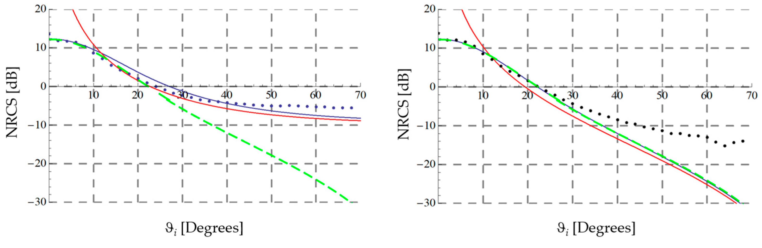
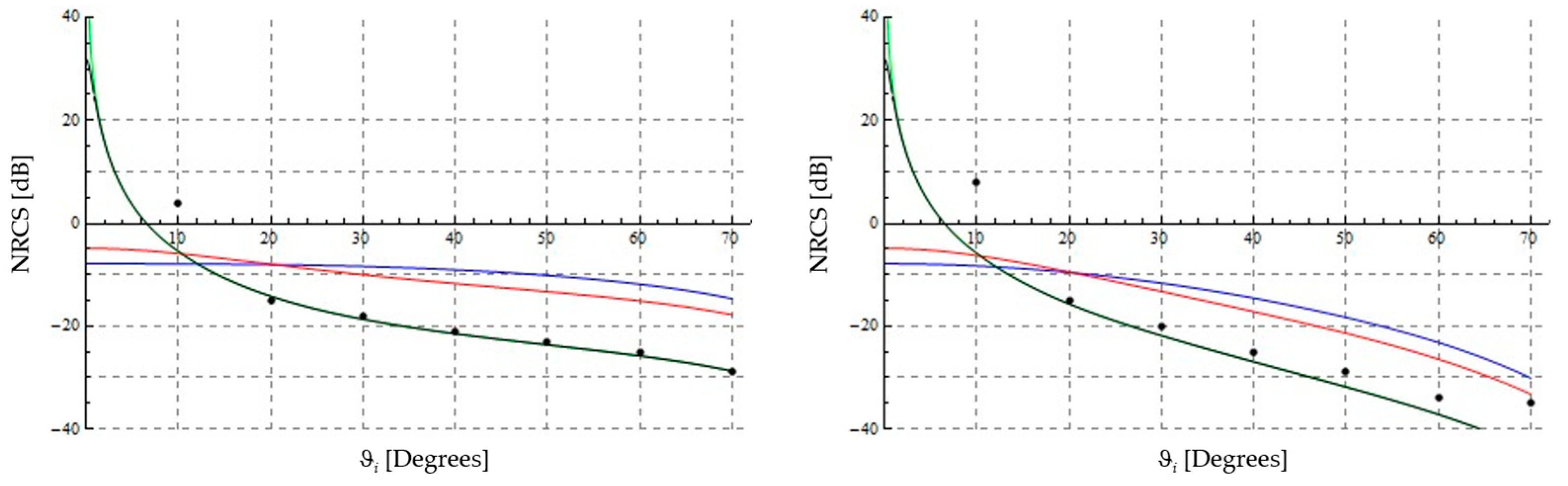
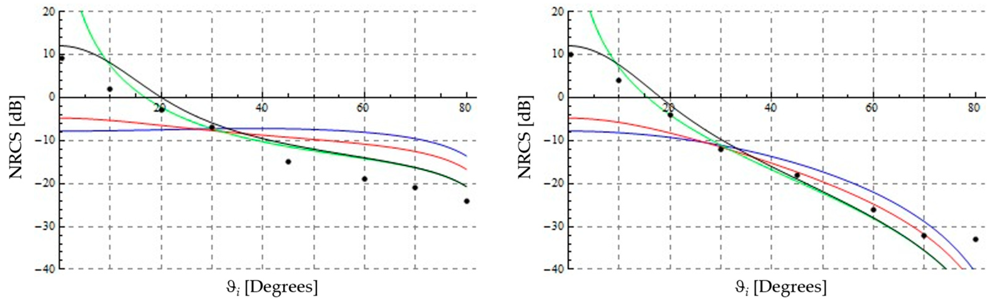
4. Numerical Results

In this section we compare the numerical results of SSA-1 for fBm surfaces with the results of SPM and KA for fBm surfaces, and with some measurements.

We first consider an artificially manufactured aluminum fBm surface, with prescribed H and $s^2$ parameters reported in the first line of

Table 1. Parameters of the surfaces considered in the comparisons with measurements.

Surface	H	s2	ε
Artificial surface [32,33]	0.7	3.6 10−3 m2−2H	~∞
Soil surface [20,34]	0.55	3.0 10−4 m2−2H	15.37–j3.71
Sea surface [1,20]	0.75	3.7 10−3 m2−2H	48.3–j34.9

. The manufacturing of this surface is described in detail in [32], and a photo of the surface is shown in Figure 4. Measurements of the backscattering NRCS of this surface, under a controlled environment, were performed at a frequency of 10 GHz for both VV and HH polarization and at several incidence angles, as described in [33]. These measurements are reported as dots in the plots of Figure 5, while SSA-1 results are reported as light-blue lines in the same figure, results of SPM and KA are also plotted for reference. We can note that, at VV polarization, the proposed SSA-1 results are in good agreement with measurements at all incidence angles, whereas KA is in good agreement with measurements only at small incidence angles and SPM is in good agreement with measurements only at large incidence angles.

It can be also noted that, at HH polarization, SSA-1 and KA results coincide. This is because in the backscattering direction for HH polarization the Bragg coefficient $B_{hh}$ appearing in the SSA-1 formulation coincides with the Fresnel reflection coefficient appearing in the KA formulation.

We want now to compare fBm SSA-1 results with backscattering measurements performed over natural scattering surfaces. In particular, we first consider a soil surface, whose measured NRCSs at 1.5 GHz and at several incidence angles, for both VV and HH polarizations, are reported in [34]. The complex relative dielectric constant of this surface, as provided in [34], is reported in the second line of Table 1, together with the parameters H and $s^2$, as determined in [20]. Comparison of measured and fBm SSA-1 backscattering NRCS values is reported in the plots of Figure 6. A very good agreement is obtained at all incidence angles, except that at 10 degrees where an underestimation of almost 10 dB is obtained. Figure 6 also shows the plots of results obtained by using SPM when applied to the fBm surface and to classical surfaces with Gaussian and exponential autocorrelation functions. These plots illustrate that fBm SSA-1 results are very similar to fBm SPM results, and that they are in much better agreement with data with respect to results obtained by SPM when applied to classical surfaces.

Finally, we consider a sea surface, whose measured NRCSs at 8.9 GHz and at several incidence angles, for both VV and HH polarizations, are reported in [1]. The complex relative dielectric constant of this surface, as provided in [1], is reported in the third line of Table 1, together with the parameters H and $s^2$, as determined in [20].

Comparison of measured and fBm SSA-1 backscattering NRCS values is reported in the plots of Figure 7. A good agreement is obtained at all incidence angles, including small ones. Figure 7 also shows the plots of results obtained by using SPM when applied to the fBm surface and to classical surfaces with Gaussian and exponential autocorrelation functions. By comparing these plots with the fBm SSA-1 ones, we can verify that fBm SSA-1 results are comparable with fBm SPM results for incidence angles greater than or equal to 10 degrees, whereas they are in much better agreement with respect to fBm SPM results at perpendicular incidence (i.e., at specular direction). In addition, fBm SSA-1 results are in much better agreement with data with respect to results obtained by SPM when applied to classical surfaces with Gaussian and exponential autocorrelation functions.

A few last words are needed on computational efficiency of the proposed method. It turns out that, with usual surface parameters of natural surfaces (see the values of $s^2$ and H in Section 2.1), at least one among series (14) and (15) converges after very few terms, except that at intermediate incidence angles where a few tens of terms are necessary. In any case, all plots in Figure 5, Figure 6 and Figure 7 are obtained in less than one second by using a commonly available laptop.

5. Conclusions

We have provided the SSA-1 formulation of the NRCS of fBm surfaces and have shown that it reduces to KA-GO and SPM formulations in their respective ranges of validity. In doing that, we have identified and fully discussed a key-parameter, i.e., Ω of (13), influencing the behavior of the obtained formulation. In addition, we have defined an effective surface slope variance, depending on frequency and viewing geometry. Our method finds application in the computation of scattering from natural (sea and soil) surfaces, which are well modeled by fBm surfaces.

The proposed formulation is fully analytical, and it does not require any numerical integration, so that it is very computationally efficient. In addition, with respect to other methods to compute scattering from power-law-spectrum surfaces, it has the advantage of not requiring the arbitrary choice of a cutoff wavenumber separating small-scale from large-scale roughness.

Presented numerical examples have shown that proposed fBm SSA-1 results are in good agreement with measurements of scattering both from an artificially manufactured fBm surface and from natural, soil and sea, surfaces. In particular, at variance with fBm SPM and fBm KA results, fBm SSA-1 results are in good agreement with measurements at both near-specular and far-from-specular directions.

The proposed method can be applied to scattering from sea surfaces at wind speeds up to about 20 m/s: at higher wind speed, unmodelled breaking waves significantly influence the scattering. This limitation is shared with KA and SPM. In addition, the proposed method can be applied to scattering from bare or sparsely vegetated soil. However, fBm surfaces are statistically isotropic, so that possible surface anisotropy cannot be accounted for by our approach in its current implementation. The extension of the fBm surface description to statistically non-isotropic surfaces is currently under study.

Finally, it must be recalled that SSA-1, just like SPM and KA, cannot account for multiple scattering and shadowing effects. This is the price to be paid for computational efficiency and simplicity of formulation.

References

1. Ulaby, F.T.; Moore, R.K.; Fung, A.K. Microwave Remote Sensing; Addison-Wesley: Reading, MA, USA, 1982; Volume II. [Google Scholar]
2. Tsang, L.; Kong, J.A.; Shin, R.T. Theory of Microwave Remote Sensing; John Wiley: New York, NY, USA, 1985. [Google Scholar]
3. Fung, A.K. Microwave Scattering and Emission: Models and Their Applications; Artech House: Norwood, MA, USA, 1994. [Google Scholar]
4. Mandelbrot, B.B. The Fractal Geometry of Nature; W.H. Freeman: New York, NY, USA, 1983. [Google Scholar]
5. Falconer, K. Fractal Geometry; John Wiley: New York, NY, USA, 1990. [Google Scholar]
6. Campbell, B.A. Scale-Dependent Surface Roughness Behavior and Its Impact on Empirical Models for Radar Backscatter. IEEE Trans. Geosci. Remote Sens. 2009, 47, 3480–3488. [Google Scholar] [CrossRef]
7. Johnson, J.T.; Shinan, R.T.; Kong, J.A.; Tsang, L.; Pak, K. A Numerical Study of the Composite Surface Model for Ocean Backscattering. IEEE Trans. Geosci. Remote Sens. 1998, 36, 72–83. [Google Scholar] [CrossRef]
8. Di Martino, G.; Iodice, A.; Riccio, D. Closed-form Anisotropic Polarimetric Two-Scale Model for fast Evaluation of Sea Surface Backscattering. IEEE Trans. Geosci. Remote Sens. 2019, 57, 6182–6194. [Google Scholar] [CrossRef]
9. Kubacki, R.; Czyżewski, M.; Laskowski, D. Minkowski Island and Crossbar Fractal Microstrip Antennas for Broadband Applications. Appl. Sci. 2018, 8, 334. [Google Scholar] [CrossRef]
10. Guariglia, E. Harmonic Sierpinski Gasket and Applications. Entropy 2018, 20, 714. [Google Scholar] [CrossRef]
11. Hwang, K.C. A Modified Sierpinski Fractal Antenna for Multiband Application. IEEE Antennas Wirel. Propag. Lett. 2007, 6, 357–360. [Google Scholar] [CrossRef]
12. Guariglia, E. Entropy and Fractal Antennas. Entropy 2016, 18, 84. [Google Scholar] [CrossRef]
13. Best, S.R. A Discussion on the Significance of Geometry in Determining the Resonant Behavior of Fractal and Other Non-Euclidean Wire Antennas. IEEE Antennas Propag. Mag. 2003, 45, 9–28. [Google Scholar] [CrossRef]
14. Krzysztofik, W.J. Fractal Geometry in Electromagnetics Applications—From Antenna to Metamaterials. Microw. Rev. 2013, 19, 3–14. [Google Scholar]
15. Li, S.J.; Cui, T.J.; Li, Y.B.; Zhang, C.; Li, R.Q.; Cao, X.Y.; Guo, Z.X. Multifunctional and Multiband Fractal Metasurface Based on Inter-Metamolecular Coupling Interaction. Adv. Theory Simul. 2019, 2, 1900105. [Google Scholar] [CrossRef]
16. Berry, M.V.; Blackwell, T.M. Diffractal Echoes. J. Phys. A Math. Gen. 1981, 14, 3101–3110. [Google Scholar] [CrossRef]
17. Yordanov, O.Y.; Ivanova, K. Kirchhoff Diffractals. J. Phys. A Math. Gen. 1994, 27, 5979–5993. [Google Scholar] [CrossRef]
18. Franceschetti, G.; Iodice, A.; Migliaccio, M.; Riccio, D. Scattering from Natural Rough Surfaces Modelled by Fractional Brownian Motion Two-Dimensional Processes. IEEE Trans. Antennas Propag. 1999, 47, 1405–1415. [Google Scholar] [CrossRef]
19. Franceschetti, G.; Iodice, A.; Riccio, D. Fractal Models for Scattering from Natural Surfaces. In Scattering; Pike, R., Sabatier, P., Eds.; Academic Press: London, UK, 2001; pp. 467–485. [Google Scholar]
20. Franceschetti, G.; Iodice, A.; Migliaccio, M.; Riccio, D. Fractals and the Small Perturbation Scattering Model. Radio Sci. 1999, 34, 1043–1054. [Google Scholar] [CrossRef]
21. Di Martino, G.; Di Simone, A.; Iodice, A.; Riccio, D. Bistatic Scattering From Anisotropic Rough Surfaces via a Closed-Form Two-Scale Model. IEEE Trans. Geosci. Remote Sens. 2021, 59, 3656–3671. [Google Scholar] [CrossRef]
22. Beckmann, P.; Spizzichino, A. The Scattering of Electromagnetic Waves from Rough Surfaces; Artech House: Norwood, MA, USA, 1987. [Google Scholar]
23. Rice, S.O. Reflection of electromagnetic waves from slightly rough surfaces. Commun. Pure Appl. Math. 1951, 4, 351–378. [Google Scholar] [CrossRef]
24. Voronovich, A.G. Small-Slope Approximation for Electromagnetic Wave Scattering at a Rough Interface of Two Dielectric Half-Spaces. Waves Random Media 1994, 4, 337–367. [Google Scholar] [CrossRef]
25. Voronovich, A.G.; Zavorotny, V.U. Full-Polarization Modeling of Monostatic and Bistatic Radar Scattering from a Rough Sea Surface. IEEE Trans. Antennas Propag. 2014, 62, 1362–1371. [Google Scholar] [CrossRef]
26. Brown, S.R.; Scholz, C.H. Broad-Band Study of the Topography of Natural Rock Surfaces. J. Geophys. Res. 1985, 90, 12575–12582. [Google Scholar] [CrossRef]
27. Austin, T.R.; England, A.W.; Wakefield, G.H. Special Problems in the Estimation of Power-Law Spectra as Applied to Topographical Modeling. IEEE Trans. Geosci. Remote Sensing 1994, 32, 928–939. [Google Scholar] [CrossRef]
28. Di Martino, G.; Iodice, A.; Riccio, D.; Ruello, G. Equivalent Number of Scatterers for SAR Speckle Modeling. IEEE Trans. Geosci. Remote Sens. 2014, 52, 2555–2564. [Google Scholar] [CrossRef]
29. Abramowitz, M.; Stegun, I.A. Handbook of Mathematical Functions; Dover: New York, NY, USA, 1970. [Google Scholar]
30. Wright, J. A New Model for Sea Clutter. IEEE Trans. Antennas Propag. 1968, 16, 217–223. [Google Scholar] [CrossRef]
31. Valenzuela, G.R. Scattering of Electromagnetic Waves from a Tilted Slightly Rough Surface. Radio Sci. 1968, 3, 1057–1066. [Google Scholar] [CrossRef]
32. Ruello, G.; Blanco, P.; Iodice, A.; Mallorqui, J.J.; Riccio, D.; Broquetas, A.; Franceschetti, G. Synthesis, Construction and Validation of a Fractal Surface. IEEE Trans. Geosci. Remote Sens. 2006, 44, 1403–1412. [Google Scholar]
33. Ruello, G.; Blanco, P.; Iodice, A.; Mallorqui, J.J.; Riccio, D.; Broquetas, A.; Franceschetti, G. Measurement of the Electromagnetic Field Backscattered by a Fractal Surface for the Verification of Electromagnetic Scattering Models. IEEE Trans. Geosci. Remote Sens. 2010, 48, 1777–1787. [Google Scholar] [CrossRef]
34. Oh, Y.; Sarabandi, K.; Ulaby, F.T. An Empirical Model and an Inversion Technique for Radar Scattering from Bare Soil Surfaces. IEEE Trans. Geosci. Remote Sens. 1992, 30, 370–381. [Google Scholar] [CrossRef]
Figure 1. Geometry of the problem.
Fractalfract 07 00387 g001
Figure 2. Plot of the function f ( ρ ) = e 1 2 k 2 u z 2 s 2 ρ 2 H ρ , for H = 0.6 (blue line), H = 0.75 (red line), and H = 0.9 (green line) showing that it is peaked for ρ ~ ρ 0 .
Fractalfract 07 00387 g002
Figure 3. Plots of Γ ( 1 / H ) Γ ( 2 / H ) (left) and a (right) vs. H, showing that these parameters are of the order of unity.
Fractalfract 07 00387 g003
Figure 4. Artificially manufactured fBm surface, see first line of Table 1.
Fractalfract 07 00387 g004
Figure 5. Plots of backscattering NRCS vs. incidence angle at 10 GHz, VV (left) and HH (right) polarizations, for the aluminum artificial fBm surface, see the first line of Table 1: measured data (black dots), SSA-1 (blue solid line), KA (green dashed line), and SPM (red solid line).
Fractalfract 07 00387 g005
Figure 6. Plots of backscattering NRCS vs. incidence angle at 1.5 GHz, VV (left) and HH (right) polarizations, for a wet soil surface, see the second line of Table 1: measured data (dots), fBm SSA-1 (black line), fBm SPM (green line), Gaussian SPM (blue line), and exponential SPM (red line). Black and green lines are practically superimposed, except at very small incidence angles. For classical surface models, surface parameters are = 0.13 and kL = 2.6.
Fractalfract 07 00387 g006
Figure 7. Plots of backscattering NRCS vs. incidence angle at 8.9 GHz, VV (left) and HH (right) polarizations, for a sea surface, see the third line of Table 1: measured data (dots), fBm SSA-1 (black line), fBm SPM (green line), Gaussian SPM (blue line), and exponential SPM (red line). For classical surface models, surface parameters are = 0.13 and kL = 2.0.
Fractalfract 07 00387 g007