Evaluation of the Methods for Nonlinear Analysis of Heart Rate Variability

Abstract

The dynamics of cardiac signals can be studied using methods for nonlinear analysis of heart rate variability (HRV). The methods that are used in the article to investigate the fractal, multifractal and informational characteristics of the intervals between heartbeats (RR time intervals) are: Rescaled Range, Detrended Fluctuation Analysis, Multifractal Detrended Fluctuation Analysis, Poincaré plot, Approximate Entropy and Sample Entropy. Two groups of people were studied: 25 healthy subjects (15 men, 10 women, mean age: 56.3 years) and 25 patients with arrhythmia (13 men, 12 women, mean age: 58.7 years). The results of the application of the methods for nonlinear analysis of HRV in the two groups of people studied are shown as mean ± std. The effectiveness of the methods was evaluated by t-test and the parameter Area Under the Curve (AUC) from the Receiver Operator Curve (ROC) characteristics. The studied 11 parameters have statistical significance (p < 0.05); therefore, they can be used to distinguish between healthy and unhealthy subjects. It was established by applying the ROC analysis that the parameters H_q=2(MFDFA), F(α)(MFDFA) and SD₂(Poincaré plot) have a good diagnostic value; H(R/S), α₁(DFA), SD₁/SD₂(Poincaré plot), ApEn and SampEn have a very good score; α₂(DFA), α_all(DFA) and SD₁(Poincaré plot) have an excellent diagnostic score. In conclusion, the methods used for nonlinear analysis of HRV have been evaluated as effective, and with their help, new perspectives are opened in the diagnosis of cardiovascular diseases.

1. Introduction

The methods of nonlinear dynamics are one of the promising tools for system analysis, which have found effective application in physics, chemistry, economics, biology, medicine, and others [1,2,3,4,5,6]. The relevance of these methods is determined by the possibility of analysis, forecasting and dynamic management of the studied processes. It is known that, for studying the nonlinear properties of cardiac signals, an important place is occupied by the analysis of the electrocardiogram, which represents the electrical activity of the heart [7,8]. The slightest deviation from the norm can mean a violation of the heart rhythm and be evidence of the presence of various diseases. One of the methods for diagnosing cardiovascular diseases is the analysis of heart rate variability (HRV). At present, the determination of HRV is recognized as one of the informative non-invasive methods for quantitative assessment of the autonomic regulation of heart rate. With the analysis of the HRV, it is possible not only to evaluate the current functional state of the human body, but also to observe its dynamics. It is believed that the reduction of HRV is due to a pathological condition of the human organism and there is a possibility of death, while high levels are registered in healthy young people, athletes [9,10]. Currently, HRV is widely used in various fields of medicine for the purpose of risk determination and diagnosis, especially in patients with cardiovascular diseases. The active study of HRV in recent years by scientists and doctors has led to the need to standardize terminology, develop optimal methods for HRV analysis, as well as determine the values of their parameters in normal and pathological conditions. This line of research has largely been initiated by the European Society of Cardiology and the North American Society of Pacing and Electrophysiology, which provides recommendations for the clinical use of HRV and creates a standard by which to assess the risk of various cardiac diseases such as angina pectoris, heart attack, life-threatening arrhythmias and others [11]. According to the created standard, the mathematical methods for the analysis of HRV fall into two main classes: linear and nonlinear. Quantitative measurements of the studied parameters when using the linear mathematical methods for analysis in the time and frequency domains have a significant clinical application, because the normal-pathology boundaries are known, according to the introduced standard. Nonlinear methods for the analysis and assessment of HRV are potentially promising tools, but they are currently in limited use because they are not standardized. The numerous scientific studies conducted in the last decade in the field of digital cardiac signals such as electrocardiograms and photoplethysmograms show that these biomedical signals include deterministic, stochastic and chaotic components [12,13,14,15]. The first and second components can be recognized by applying the methods of linear analysis, while the analysis of the chaotic properties of signals causes certain difficulties related to the need to use methods of the nonlinear dynamics. The nonlinear chaotic dynamics give the body many functional advantages. Systems that exhibit a certain amount of chaos are capable of operating in a wide range of conditions and therefore easily adapt to changes in the environment. Chaotic behavior externally manifests itself in data variability. The decrease in variability is a manifestation of pathological changes in the human body. Thus, for example, in a publication [16] it is reported that heart rate variability decreases compared to the norm for several seconds and sometimes for several months before the occurrence of a cardiac arrest. Therefore, timely measurement of the parameters of the chaotic behavior of cardiac signals can facilitate the task of diagnosing the patient’s condition and reduce the likelihood of serious illness or death. The authors of [17] declared the reduced HRV and increased probability of death after myocardial infarction. Their conclusions are based on a studied group of patients who experienced myocardial infarction and subsequent death.

In recent years, fractal and multifractal methods have been used for the analysis of cardiac time series [18,19,20,21,22], which take into account the dynamics of the heart rhythm. Their distinguishing feature is that, together with the global characteristics of the process, they also allow revealing the peculiarities of their local structure. An important characteristic of these time series is the fractal dimension D=2-H, where H is the Hurst exponent, which is one of the key indicators characterizing fractal processes [23]. The values of this parameter are in the interval (0, 1). When the value of the Hurst exponent is greater than 0.5 and less than 1.0 (0.5 < H < 1.0), these processes have a stable behavior (maintaining the existing trend). The higher the value of this parameter and it approaches 1.0, the stronger the tendency and the process approaches a state of determinism and full predictability. In the case that H = 0.5, the process consists of random and uncorrelated increments. Such a process is called “white noise” and is characterized by maximum chaos and minimum predictability. If the value of the Hurst exponent is 0 < H < 0.5, this process is called antipersistent, which means that its increase in the past means a decrease in the future and vice versa. The value of the Hurst exponent of the fractal processes is 0.5 < H < 1.0, and it can be determined by applying the statistical methods [24]. The fractal processes are characterized by the following two properties: self-similarity and fractal dimensionality. A fractal process is self-similar if it can be decomposed into smaller parts, each of which is similar to the main one. The fractal dimension takes fractional values and lies between the Euclidean and topological dimensions. The fractal processes are of two main types: monofractal and multifractal. The monofractal process is described by a single value of the Hurst parameter/fractal dimension, while the multifractal process is described by a spectrum of values of the Hurst parameter/fractal dimension [25]. The fractal and multifractal analyses provide new opportunities for studying the nonlinear cardiac signals by applying the following methods: Detrended Fluctuation Analysis (DFA) and Multifractal Detrended Fluctuation Analysis (MFDFA). These nonlinear methods are based on the assumption that the interval series between heartbeats (RR time intervals) possess characteristics related to fractal geometry, such as self-similarity, scalability, fractal dimension.

Another important characteristic of dynamical systems is entropy, which provides an estimate of the complexity and predictability of the time series [26,27]. The entropy value gives information on how far the system is from an ordered, structured state and how close it is to a completely chaotic, structureless, homogeneous form.

The application of nonlinear graphical methods, such as the Poincaré plot for the analysis of HRV, provides visual information about the physiological state of patients and opens up additional opportunities for clinical and research applications [28].

Despite the wide use of HRV in studying the state of the cardiovascular system of patients by applying linear methods, and in recent years also using nonlinear methods, there remain a number of unsolved problems related to the correct interpretation of the results of nonlinear analysis, which requires research in this area to continue. It has been suggested that nonlinear analysis methods can provide important information about the physiological state as well as cardiovascular disease risk assessment, but there is a problem related to determining which nonlinear methods are most informative and what the values of the studied parameters are in healthy and diseased subjects.

The purpose of the present article is to solve the problems mentioned above in the study of the fractal, multifractal, visual and informational properties of the intervals between heartbeats of two groups of people: healthy individuals and patients with arrhythmia. The research was conducted by applying the following nonlinear analysis methods: Rescaled Range, Detrended Fluctuation Analysis, Multifractal Detrended Fluctuation Analysis, Poincaré plot, Approximate Entropy and Sample Entropy. The efficiency of the used nonlinear methods will be evaluated by means of the t-test and the parameter Area Under the Curve (AUC) from the Receiver Operator Curve (ROC) characteristics. Based on the obtained results, a diagnostic assessment of the methods used will be done.

2. Materials and Methods

To analyze and evaluate the informational characteristics of the internal organization of the intervals between heartbeats (RR interval series), it is expedient to use methods of nonlinear dynamics, which are grouped into the following categories:

• Fractal and multifractal methods: Rescaled Range (R/S), Detrended Fluctuation Analysis (DFA) and Multifractal Detrended Fluctuation Analysis (MFDFA;
• Visual methods: Poincaré plot;
• Information methods: Approximate Entropy (AppEn) and Sample Entropy (SampEn).

2.1. Fractal and Multifractal Methods

2.1.1. R/S Method

To study self-similar (fractal) processes, statistical methods can be used to determine the value of the Hurst exponent. R/S is one of the most commonly used statistical methods. This method was proposed by the English researcher Hurst, who discovered that the data on the flooding of the Nile River over a long period of time (800 years) were randomly scattered around a straight line with a slope of H > 1/2, and this was defined as the effect of Hurst [29]. Although the method was created a long time ago, it is still used today in the analysis of fractal processes in various fields of science; as proof of this are numerous publications [24,30,31,32,33].

The main steps of the R/S method are:

Step 1:

The investigated process is divided into segments of different lengths.

Step 2:

For each segment, the parameters are calculated: Range R(n) and standard deviation S(n) with the following formulas:

• Range R(n):

  $$\mathrm{R}\left(\mathrm{n}\right)=\max \left(0,{\mathrm{W}}_1,\dots ,{\mathrm{W}}_{\mathrm{n}}\right)-\min \left(0,{\mathrm{W}}_1,\dots ,{\mathrm{W}}_{\mathrm{n}}\right),$$

  (1)

  where:

  $$W_j=\left({\mathrm{X}}_1+{\mathrm{X}}_2+\dots +W_j\right)-\mathrm{j}\overline{\mathrm{X}\left(\mathrm{n}\right)}, \mathrm{j}=1, 2, \dots , \mathrm{n}.$$

  (2)
• Standard deviation S(n):

  $$\mathrm{S}\left(\mathrm{n}\right)=\sqrt{\mathrm{E}{\left({\mathrm{X}}_{\mathrm{j}}-\mathsf{\mu }\right)}^2,} \mathsf{\mu } \mathrm{is} \mathrm{the} \mathrm{mean} \mathrm{of} ({\mathrm{X}}_1, \dots , {\mathrm{X}}_{\mathrm{j}}).$$

  (3)

Step 3:

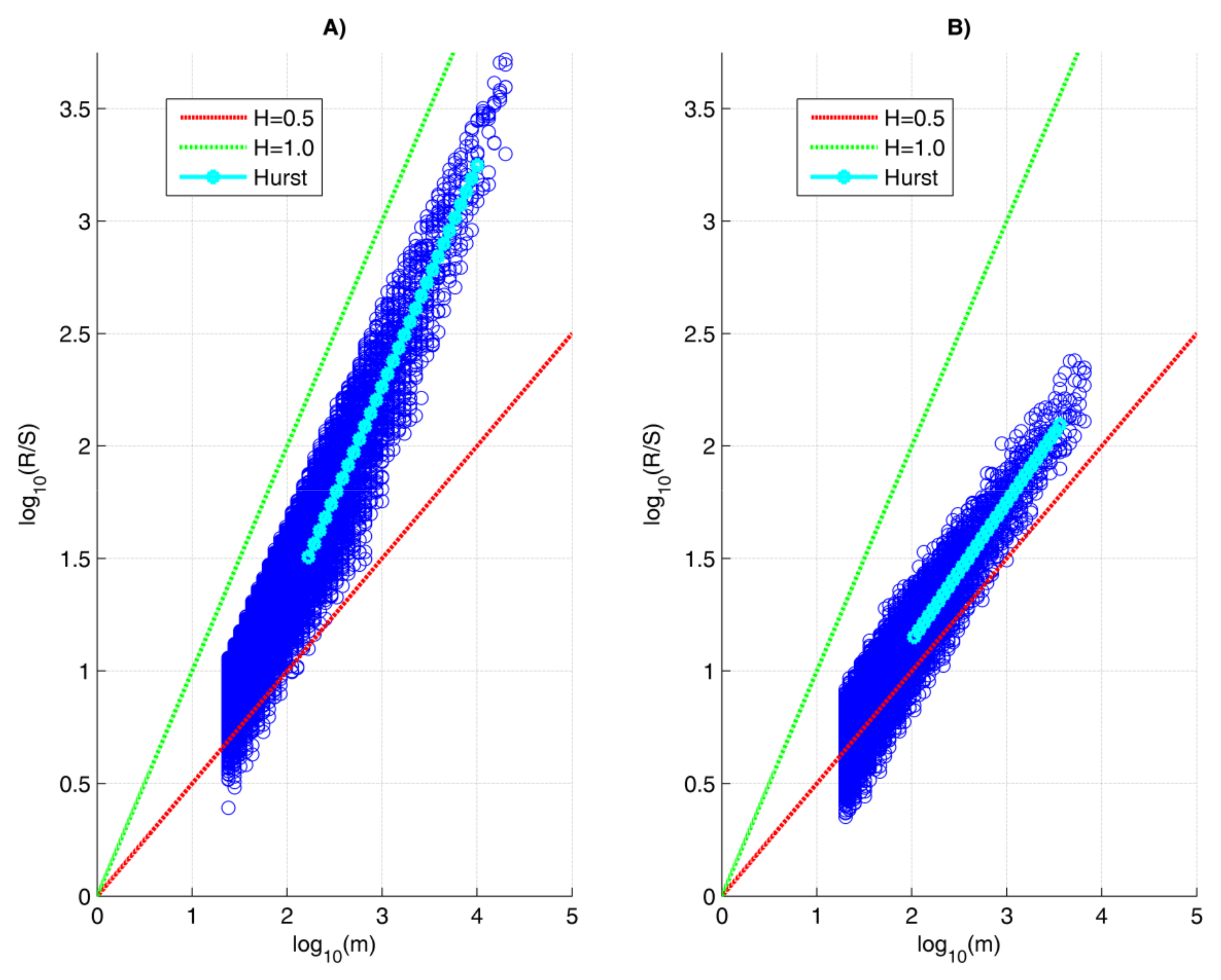
The relationship between R(n) and S(n) is determined. A regression model between Log₁₀(R/S) and Log₁₀(segment size) is created. For fractal processes, the relationship between these two variables is linear.

Step 4:

Using the method of least squares, the slope of the regression line is determined.

Step 5:

The value of the Hurst exponent is determined, which is equal to the slope of the regression line.

$$\mathrm{H}=\mathsf{\beta }$$

(4)

where β is the slope of the regression line.

2.1.2. Detrended Fluctuation Analysis Method

The DFA is a suitable method for studying the fractal properties of cardiac signals (RR interval series). This method is described in publications [34,35,36,37,38,39].

The method uses the following parameters:

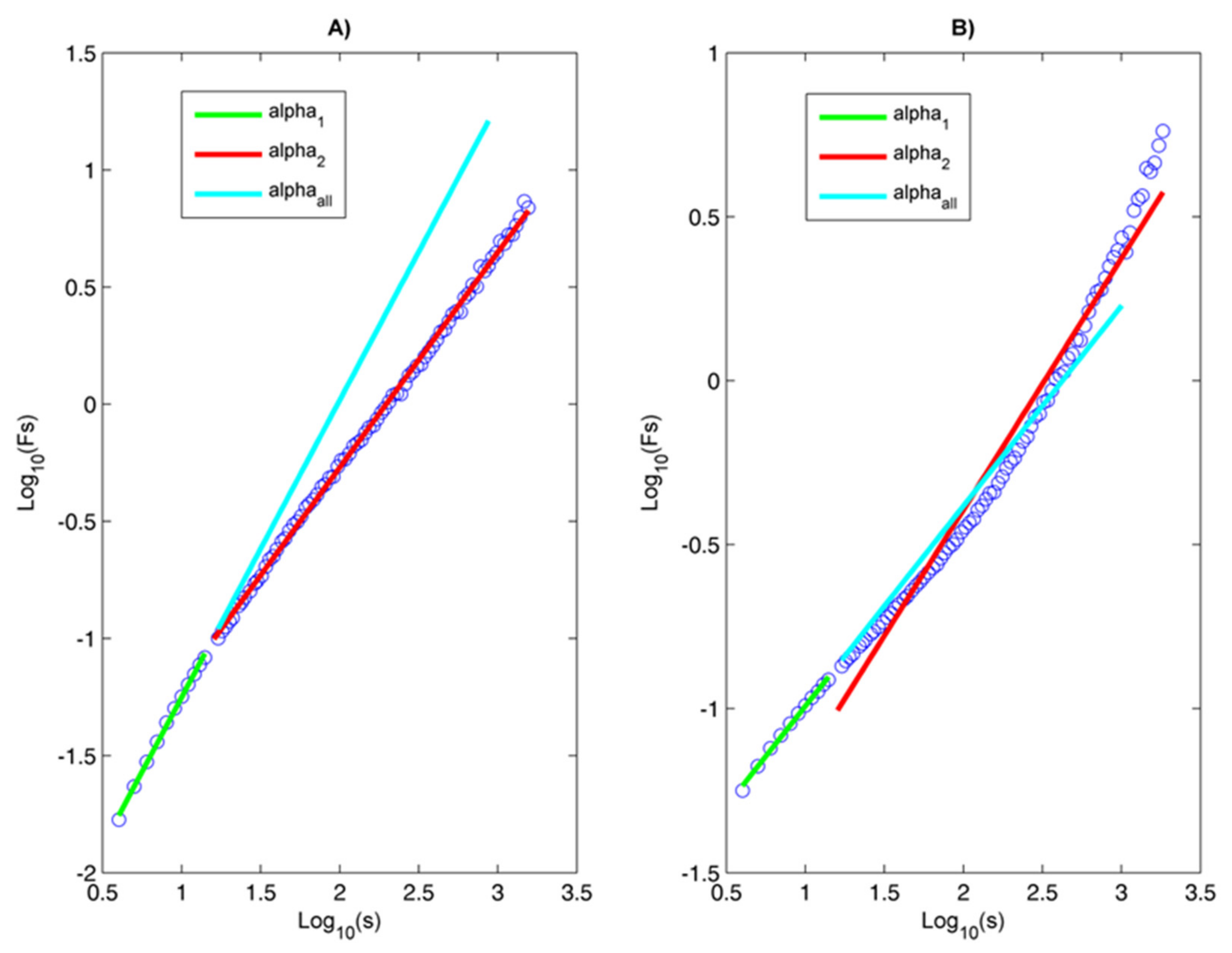
• α₁ to detect short-term correlations;
• α₂ to detect long-term correlations;
• α_all to detect the self-similarity in the signal. If it has a value of 0.5, it is an indicator of an uncorrelated process resembling white noise, while if the value of α_all is between 0.5 and 1, it is evidence of positive correlations and self-similarity (fractality) in the process. Conversely, if the process has a value for α_all that is between 0 and 0.5, this is an indication of negative correlations. Using the DFA method, the coefficient of fluctuations of the process can be determined, which is related to the Hurst exponent. When the value of the parameter α_all is less than or equal to 1, the resulting value of α_all coincides with the value of the Hurst exponent.

The procedure for applying the DFA method consists of the following main steps:

Step 1:

For the analyzed time series X(i), i = 1, 2, …, N, a fluctuation profile with an average value $\overline{x }$ is determined:

$$\mathrm{Y}\left(\mathrm{i}\right)={\sum }_{k=1}^i[x\left(k\right)-\overline{x]}.$$

(5)

Step 2:

The resulting time series Y(i) is divided into Ns = int(N/s) non-overlapping segments containing an equal number of points s. In case the length of the time series N is not a multiple of s, the division procedure is repeated starting from the opposite end of the series. This results in 2N segments of length s.

Step 3:

The local trend for each segment is calculated using the method of least squares and the sums for the segments v = 1, N and v = N_s + 1, …, 2N are determined:

$${ \mathrm{F}}^2\left(\mathrm{v},\mathrm{s}\right)=\frac{1}{\mathrm{s}}{\sum }_{\mathrm{i}=1}^{\mathrm{s}}{\left\{\mathrm{Y}\left[\left(\mathrm{v}-1\right)\mathrm{s}+\mathrm{i}\right]-{\mathrm{y}}_{\mathrm{v}}\left(\mathrm{i}\right)\right\}}^2$$

(6)

$${ \mathrm{F}}^2\left(\mathrm{v},\mathrm{s}\right)=\frac{1}{\mathrm{s}}{\sum }_{\mathrm{i}=1}^{\mathrm{s}}{\left\{\mathrm{Y}\left[\mathrm{N}-\left(\mathrm{v}-{\mathrm{N}}_{\mathrm{s}}\right)\mathrm{s}+\mathrm{i}\right]-{\mathrm{y}}_{\mathrm{v}}\left(\mathrm{i}\right)\right\}}^2.$$

(7)

Step 4:

A summation is performed for all segments, resulting in the following fluctuation function:

$$\mathrm{F} \left(\mathrm{s}\right)={\left\{\frac{1}{2{\mathrm{N}}_{\mathrm{s}}}{\sum }_{\mathrm{v}=1}^{2{\mathrm{N}}_{\mathrm{s}}}{\mathrm{F}}^2\left(\mathrm{v},\mathrm{s}\right)\right\}}^{1/2}.$$

(8)

Step 5:

Steps 2 to 4 are repeated for different values of the parameter s. The fluctuation function is determined:

$$\mathrm{F}\left(\mathrm{s}\right)~{\mathrm{s}}^{\mathsf{\alpha }}.$$

(9)

According to Equation (9), the linear behavior of the function F(s) indicates the presence of scaling (self-similarity).

2.1.3. Multifractal Detrended Fluctuation Analysis Method

The MFDFA method is used to analyze the complexity and heterogeneity of the studied time series based on the scaling behavior. The application of this method in the analysis of RR intervals aims to extract its fractal/multifractal characteristics that reflect changes in the behavior of cardiac signals and to identify the pathological conditions of the patient, if any, in order to make the correct diagnosis.

The implementation of the algorithm is described in publications [28,40,41,42,43,44]. The first three steps of MFDFA are the same as in the DFA method, and the next three steps are as follows:

Step 4:

The F_q(s) function is determined for the following two cases: q ≠ 0; q → 0.

$${ \mathrm{F}}_{\mathrm{q}}\left(\mathrm{s}\right)={\left\{ \frac{1}{2{\mathrm{N}}_{\mathrm{s}}}\left.{\sum }_{\mathrm{v}=1}^{2{\mathrm{N}}_{\mathrm{s}}}{[{\mathrm{F}}^2\left(\mathrm{v},\mathrm{s}\right)]}^{\mathrm{q}/2}\right\} \right.}^{1/\mathrm{q}} \mathrm{for} \mathrm{q} \ne 0$$

(10)

$${ \mathrm{F}}_0\left(\mathrm{s}\right)=\exp \left\{ \frac{1}{4{\mathrm{N}}_{\mathrm{s}}}\left.{\sum }_{\mathrm{v}=1}^{2{\mathrm{N}}_{\mathrm{s}}}\ln [{\mathrm{F}}^2\left(\mathrm{v},\mathrm{s}\right)]\right\} \right. \mathrm{for} \mathrm{q} \to 0$$

(11)

Step 5:

For a fixed value of q, the graphical dependence of log Fq(s) vs. log(s) is plotted. If the studied time series has a fractal behavior, then Fq(s) changes according to the power law:

$${ \mathrm{F}}_{\mathrm{q}}\left(\mathrm{s}\right)~{\mathrm{s}}^{\mathrm{h}\left(\mathrm{q}\right)}.$$

(12)

where h(q) is called the generalized Hurst exponent.

Step 6:

For different values of the parameter q, steps 1 to 5 are repeated.

When studying the scalable properties of the time series, it is convenient to move from the generalized Hurst exponent h(q) to the scalable exponent τ(q) and the multifractal spectrum f(α) [2,6]:

$$\tau \left(\mathrm{q}\right)=\mathrm{qh}\left(\mathrm{q}\right)-1.$$

(13)

F(α) = qα − τ(q), α = τ^’(q).

(14)

The monofractal processes are characterized by the following properties:

• The fluctuation function F_q(s) is the same for all segments v into which the studied process is divided;
• The generalized Hurst exponent h(q) = H does not depend on the parameter q and is a constant quantity;
• They are characterized by a linear increase of the function τ(q);
• They have a narrow multifractal spectrum F(α).

The multifractal processes have the following features:

• The fluctuation function F_q(s) is different for the different segments v into which the process is divided;
• The generalized Hurst exponent is not a constant quantity, but depends on the change of the parameter q;
• The function τ(q) increases nonlinearly;
• The multifractal spectrum F(α) is wide.

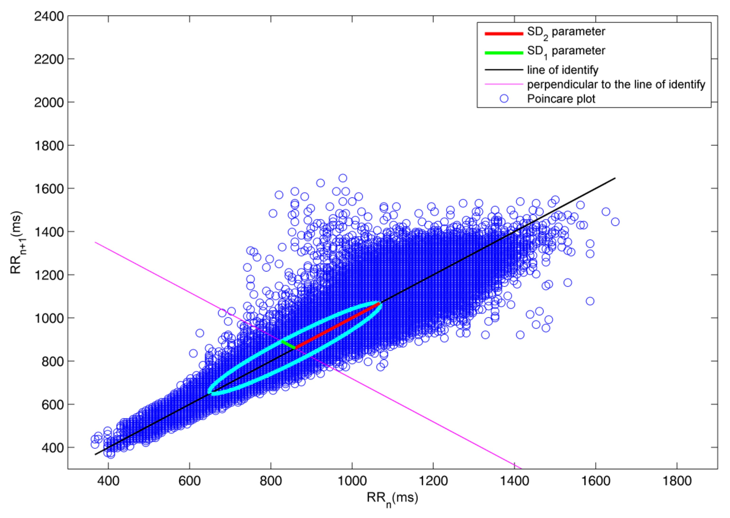
2.2. Poincaré Plot

The Poincaré plot is a two-dimensional visualization tool for dynamic cardio intervals (previous and next RR interval), which form a “cloud” of points [7,28]. This method is used to demonstrate the self-similarity of the heartbeat. If an ellipse with a longitudinal axis (the line of identity) and a transverse axis (perpendicular to the line of identity) is constructed on the graph constructed by the Poincaré method (Figure 1), the following parameters can be determined:

• SD₂ [ms] parameter, which corresponds to the semimajor axis of the ellipse and lies on a line that is perpendicular to the line of identity. This parameter corresponds to the long-term variability of the RR intervals;
• SD₁ [ms] parameter, which corresponds to the semiminor axis of the ellipse and lies on the line of identity. This parameter is related to the rapid variations between heartbeats;
• The SD₁/SD₂ ratio, which shows the relationship between the short- and long-term HRV.

The parameters characterizing the Poincaré method are determined by the following equations [13]:

$$\mathrm{x}=\left\{{\mathrm{x}}_1,{\mathrm{x}}_2,\dots ,{\mathrm{x}}_{\mathrm{n}}\right\}=\left\{{\mathrm{RR}}_1,{\mathrm{RR}}_2,\dots ,{\mathrm{RR}}_{\mathrm{n}}\right\},$$

(15)

$$\mathrm{y}=\left\{{\mathrm{y}}_1,{\mathrm{y}}_2,\dots {\mathrm{y}}_{\mathrm{n}}\right\}=\left\{{\mathrm{RR}}_2,{\mathrm{RR}}_3,\dots ,{\mathrm{RR}}_{\mathrm{n}+1}\right\},$$

(16)

$${ \mathrm{SD}}_1=\sqrt{\mathrm{var}\left({\mathrm{d}}_1\right)},{ \mathrm{SD}}_2=\sqrt{\mathrm{var}\left({\mathrm{d}}_2\right)}.$$

(17)

where:

• $\mathrm{i}=1,2,\dots ,\mathrm{n},$ n are the number of points in the graph;
• var(d) is the variance of d;
• ${\mathrm{d}}_1=\frac{\mathrm{x}-\mathrm{y}}{\sqrt{2}}$; ${\mathrm{d}}_2=\frac{\mathrm{x}+\mathrm{y}}{\sqrt{2}}$.

One of the features for visual analysis of HRV that is used in the present study is determined by the shape that the points of the “cloud” form. Figure 2 shows several patterns that are categorized for different functional states of the study subjects [42]:

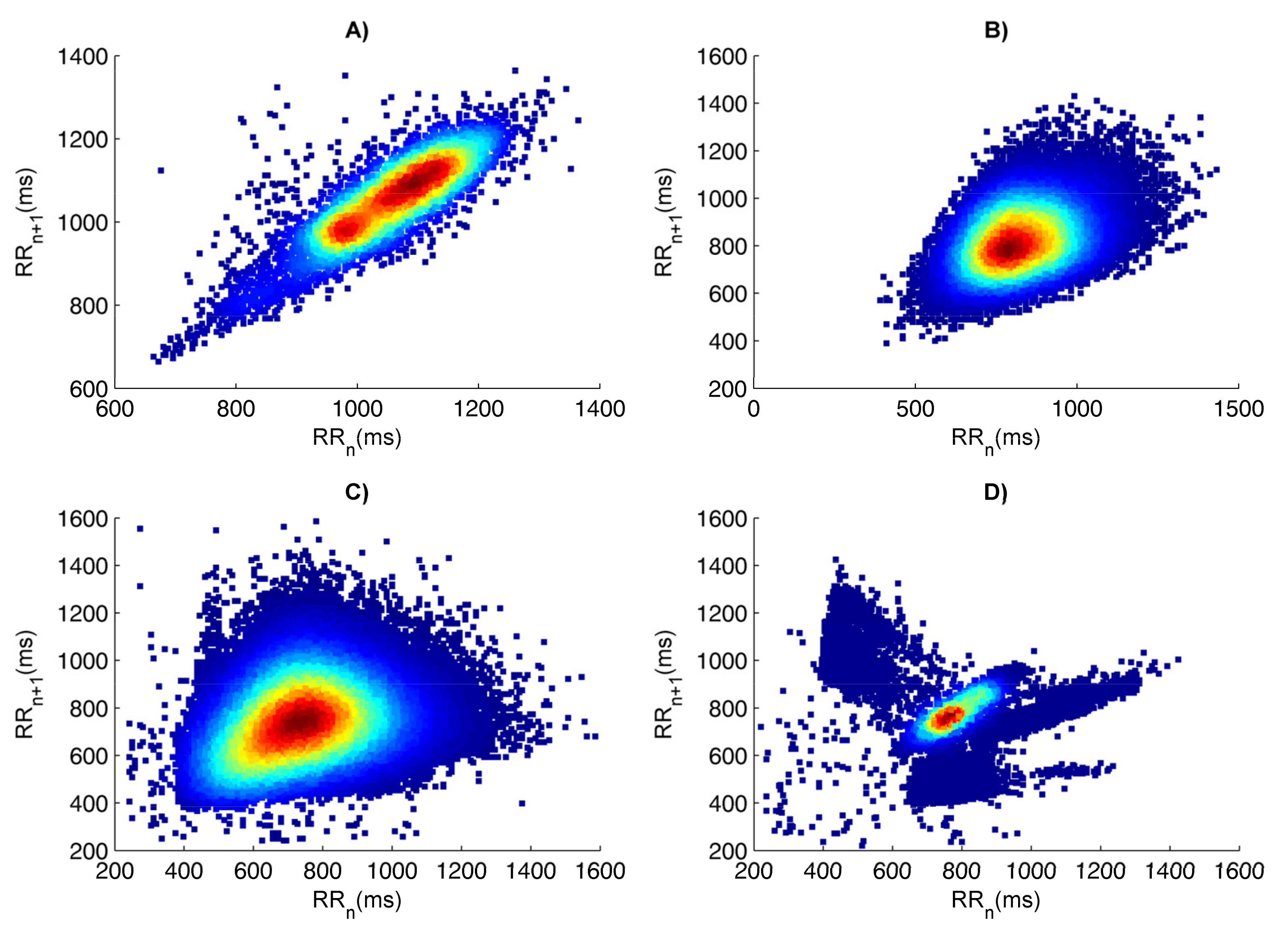
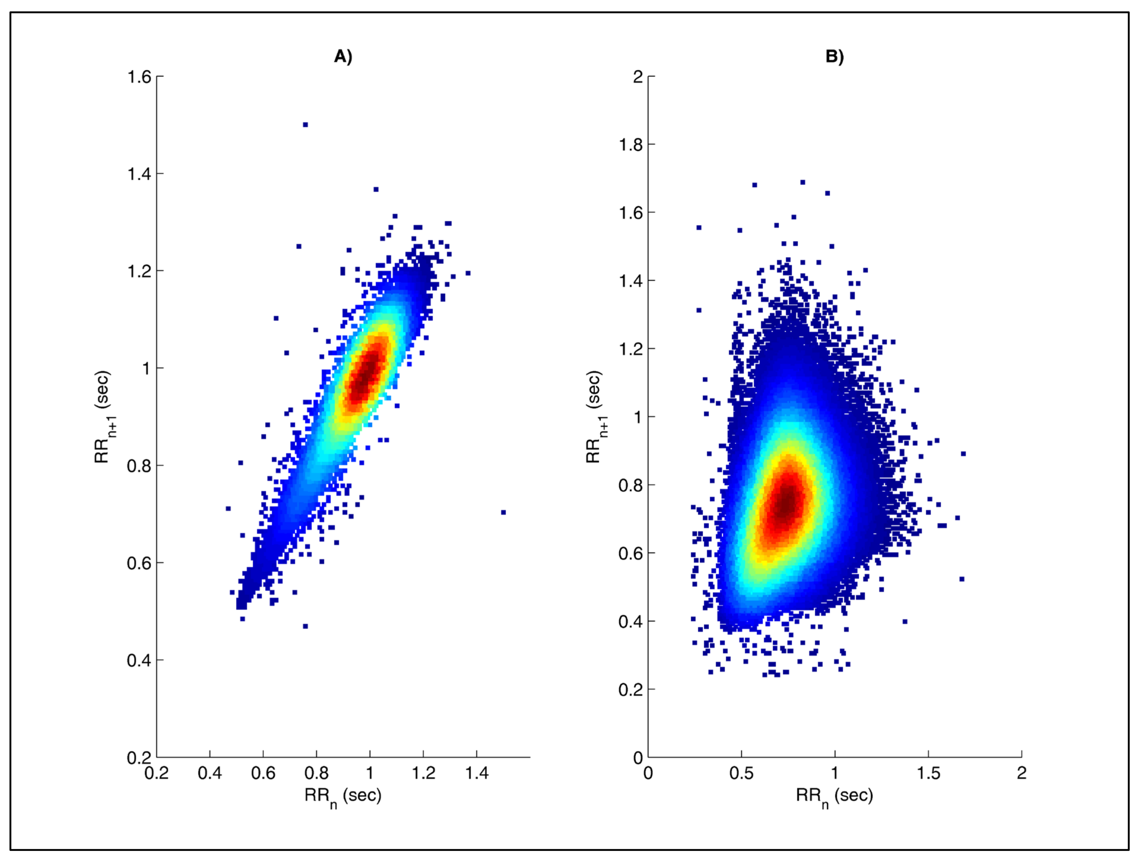
• The graph of the healthy subject has one main segment of points to which more points may be evenly scattered. The main segment is comet-shaped with a narrow lower part and gradually widening towards the apex (Figure 2A);
• The graph of the diseased subject has the shape of a torpedo (Figure 2B), a fan (Figure 2C) or a complex shape (consisting of several segments), depending on the type of disease (Figure 2D).

The graph constructed using the Poincaré plot can be analyzed quantitatively by placing an ellipse on the graph shape and determining the values of the parameters: SD₁, SD₂ and SD₁/SD₂ ratio.

2.3. Approximate Entropy and Sample Entropy

Approximate entropy (ApEn) [26,44,45,46,47] serves as a quantitative measure of regularity, predictability and complexity of nonstationary time series such as RR interval series. This entropy depends on the following 3 factors:

• Subseries length (m);
• Tolerance (r);
• Data length (N).

To calculate the entropy for a time series of N points, Vectors (18) and (19) are first constructed, and then the entropy is calculated with Formula (20).

$$\mathrm{y}\left(\mathrm{i}\right)=\left[\mathrm{x}\left(\mathrm{i}\right),\dots ,\mathrm{x}\left(\mathrm{i}+\mathrm{m}-1\right)\right].$$

(18)

$$\mathrm{y}\left(\mathrm{j}\right)=\left[\mathrm{x}\left(\mathrm{j}\right),\dots ,\mathrm{x}\left(\mathrm{j}+\mathrm{m}-1\right)\right].$$

(19)

$$\mathrm{ApEn}\left(\mathrm{m},\mathrm{r},\mathrm{N}\right)={\mathsf{\varphi }}^{\mathrm{m}}\left(\mathrm{r}\right)-{\mathsf{\varphi }}^{\mathrm{m}+1}\left(\mathrm{r}\right).$$

(20)

where:

• ${\mathsf{\Phi }}^{\mathrm{m}}\left(\mathrm{r}\right)=\frac{1}{\mathrm{N}-\mathrm{m}+1}{\displaystyle \sum }_{\mathrm{i}=1}^{\mathrm{N}-\mathrm{m}+1}{\mathrm{lnC}}_{\mathrm{i}}^{\mathrm{m}}\left(\mathrm{r}\right);$
• ${\mathrm{C}}_{\mathrm{i}}^{\mathrm{m}}\left(\mathrm{r}\right)=\frac{\mathrm{number} \mathrm{of} \mathrm{y}\left(\mathrm{j}\right);\mathrm{d}\left[\mathrm{y}\left(\mathrm{i}\right), \mathrm{y}\left(\mathrm{j}\right)\right]\le \mathrm{r}}{\mathrm{N}-\mathrm{m}+1};$
• d is the distance between the vectors.

It is found that the higher the regularity of the signal, the lower the entropy, and for irregular signals, the entropy is higher.

SampEn is a modification of ApEn used to estimate the complexity of physiological time series [45]. This entropy is very similar to ApEn with minor computational differences. To determine SampEn, it is necessary to define ${\mathsf{\varphi }}^{\mathrm{m}}\left(r\right)$ and ${\mathsf{\varphi }}^{\mathrm{m}+1}\left(r\right)$.

$${\mathsf{\varphi }}^{\mathrm{m}}\left(r\right)=\frac{1}{\mathrm{N}-\mathrm{m}}{\sum }_{\mathrm{i}=1}^{\mathrm{N}-1}{\mathrm{C}}_{\mathrm{i}}^{\mathrm{m}}\left(\mathrm{r}\right).$$

(21)

$$\mathrm{SampEn}\left(\mathrm{m},\mathrm{r},\mathrm{N}\right)=\ln \frac{{\mathsf{\varphi }}^{\mathrm{m}}\left(\mathrm{r}\right)}{{\mathsf{\varphi }}^{\mathrm{m}+1}\left(\mathrm{r}\right)}.$$

(22)

The probability ${\mathsf{\varphi }}^{\mathrm{m}}(\mathrm{r}$) that two sequences match for m points is calculated by determining the average number of vector pairs for which the distance between them is less than the parameter r. In a similar way, the variability ${\mathsf{\varphi }}^{\mathrm{m}+1}\left(\mathrm{r}\right)$ is determined.

Characteristic of SampEn is that, unlike ApEn, it does not depend on the length of the data.

2.4. Data

The data used for the research in this article were recorded with a Dynamic ECG Systems TLC9803 Holter device at the Medical University of Varna, Bulgaria. A cardiologist was involved in registering the data and made the relevant diagnoses. The studied RR time series are of 50 subjects, who are united in the following 2 groups:

• Group 1 (healthy subjects) consisted of 25 subjects, of which 15 were male and 10 were female. The average age for this group is 56.3 years.
• Group 2 (arrhythmia patients) consisted of 25 patients, of which 13 were men and 12 were women. The average age of the group is 58.7 years.

The group corresponding to patients with arrhythmia included only subjects with supraventricular extrasystoles. During the study, patients were not taking antiarrhythmic medications, including beta-selective blockers.

MATLAB (R2013b version) software was created to analyze 24 h recordings consisting of approximately 100,000 RR intervals.

2.5. Receiver Operating Characteristics Analysis

In the present article, to determine the diagnostic evaluation of the proposed methods for the nonlinear analysis of the HRV, the t-test and ROC analysis using MedCalc software is applied [48]. ROC analysis is a classic methodology from the signal theory that is currently widely used in medical diagnostics. This statistical method is based on the construction of ROC curves, which do not work with absolute indicators of the correct classification of results, but with relative indicators such as sensitivity and specificity. Sensitivity is the proportion of positive cases that were correctly classified by the model, while specificity is the proportion of negative cases.

The area under the ROC curve (AUC parameter) is a measure of how well a parameter can discriminate between two diagnostic groups. The relationship between the quality of the method used and the AUC value is as follows:

• If the AUC is in the interval 0.9–1.0, the quality of the parameter used is excellent;
• If the AUC is in the interval 0.8–0.9, the quality of the parameter used is very good;
• If the AUC is in the interval 0.7–0.8, the quality of the parameter used is good;
• If the AUC is in the interval 0.5–0.6, the quality of the method used is unsatisfactory.

3. Results and Discussion

3.1. Evaluation of the Fractal and Multifractal Methods for the Analysis of HRV

3.1.1. Evaluation of the R/S Method

The graphs obtained by the R/S method for determining the Hurst exponent are shown in Figure 3A (healthy subject) and Figure 3B (arrhythmic patient). The slopes of the charts, colored in light blue, correspond to the Hurst exponent values. The value of this parameter for a healthy individual is H = 0.956, and for a patient with arrhythmia it is H = 0.681. The determined values (mean ± std) of the Hurst exponent for the studied two groups of subjects are shown in

Table 1. Comparative analysis between healthy (Group 1) and unhealthy subjects (Group 2).

Parameters	Group 1 (Mean ± Std)	Group 2 (Mean ± Std)	AUC	95% Confidence Interval	p-Value
Fractal and Multifractal Methods
H (R/S)	0.981 ± 0.01	0.701 ± 0.07	0.852	0.721 to 0.937	<0.0001
α1 (DFA)	1.106 ± 0.21	0.723 ± 0.18	0.879	0.754 to 0.955	<0.0001
α2 (DFA)	1.042 ± 0.08	0.805 ± 0.07	0.926	0.814 to 0.981	<0.0001
αall (DFA)	0.973 ± 0.02	0.745 ± 0.03	0.918	0.791 to 0.972	<0.0001
Hq=2 (MFDFA)	0.978 ± 0.04	0.699 ± 0.06	0.789	0.638 to 0.886	<0.0001
F(α) (MFDFA)	0.550 ± 0.18	0.201 ± 0.05	0.798	0.660 to 0.898	<0.0001
Poincaré plot
SD1 [ms]	29.12 ± 10.19	145.46 ± 31.01	0.925	0.814 to 0.980	<0.0001
SD2 [ms]	175.15 ± 41.22	210.70 ± 25.12	0.725	0.580 to 0.842	0.0006
SD1/SD2	0.141 ± 0.11	0.723 ± 0.13	0.863	0.736 to 0.944	<0.0001
Entropy Methods
ApEn	1.592 ± 0.15	1.212 ± 0.19	0.832	0.700 to 0.923	<0.0001
SampEn	1.697 ± 0.21	1.351 ± 0.20	0.876	0.752 to 0.952	<0.0001

. It was found that, for the two studied groups, the value of the Hurst parameter was in the interval (0.5, 1.0), which is evidence that these signals have a fractal behavior. The value of this parameter is lower in patients with arrhythmia. In a number of scientific studies, it has been found that the Hurst exponent decreases with fatigue, physical exertion and cardiovascular diseases, and from this, the HRV also decreases [23,49]. A similar trend was found in the present study, confirming the adverse impact of cardiovascular arrhythmia on HRV.

The estimation of this parameter was determined by applying the t-test and ROC analysis. Using the t-test, it was established that the Hurst parameter, determined by the R/S method, has statistical significance (p < 0.05), which allows to delineate the two studied groups. The ability of ROC analysis to discriminate diseased from healthy individuals was determined by examining the area under the ROC curve (AUC), as the numerical values in Table 1. The diagnostic evaluation of the R/S method based on the determined AUC value was established as very good.

3.1.2. Evaluation of the DFA Method

To study the RR time intervals using the DFA method, the values of the parameters α₁, α₂ and α_all are determined. Figure 4A,B shows DFA plots of RR time intervals for a healthy subject and an arrhythmia patient. The α₁ parameter is determined by the slope of the first part of the graph (colored in green). This parameter is defined for segments of size 4 ≤ s < 16 and corresponds to the short-term variations of the signal. The parameter α₂ is determined by the slope of that part of the graph, which is colored red. This parameter is defined for segments of size 16 ≤ s < 64 and corresponds to the long-term signal variations. The parameter α_all is determined by the slope of the graph, which is colored in light blue. The values of the studied parameters (α₁, α₂ and α_all) for both types of signals are shown in Table 1. The results obtained show the following:

• The values of α₁, α₂ and α_all are higher in healthy people;
• The value of the parameter α_all in healthy and diseased subjects varies between 0.5 and 1.0, which is close to the value of the Hurst exponent determined by the R/S method;
• The parameters α₁, α₂ and α_all have statistical significance determined by t-test; therefore, with this method, the two groups can be distinguished;
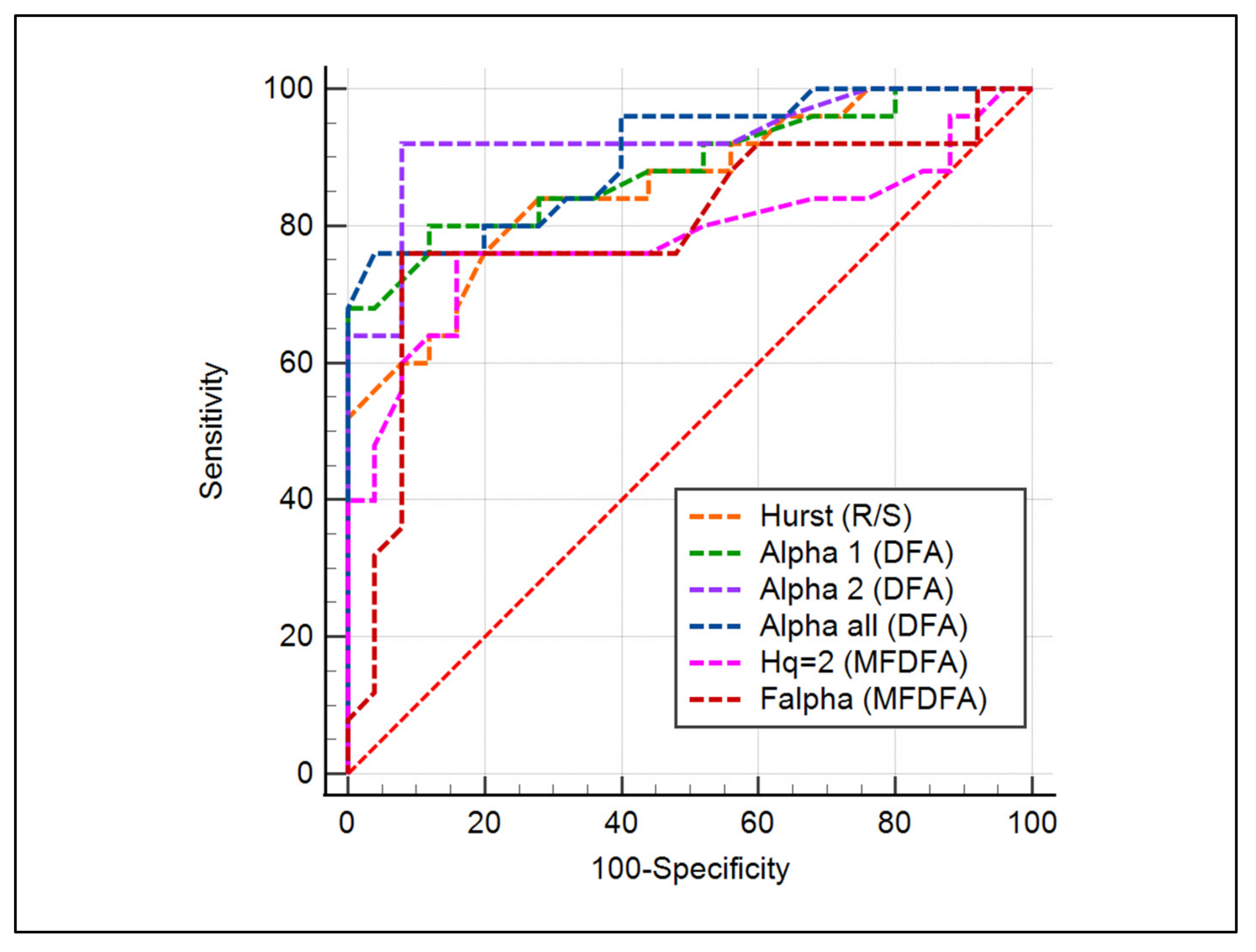
• Quantitative AUC evaluation shows that one of the parameters (α₁) has a very good diagnostic score and the other two (α₂ and α_all) have an excellent score. Quantitative AUC evaluation shows that one of the parameters (α₁) has a very good diagnostic score, and the other two (α₂ and α_all) have an excellent score; the graphs for the three parameters obtained by the ROC analysis are shown in Figure 5.

3.1.3. Evaluation of the MFDFA Method

The estimation of the degree of fractality of the RR time intervals is an important feature when studying their fluctuations in order to obtain information about the long-term correlations and, accordingly, to determine and predict the behavior of these intervals. Based on the analyses, the following conclusions can be drawn:

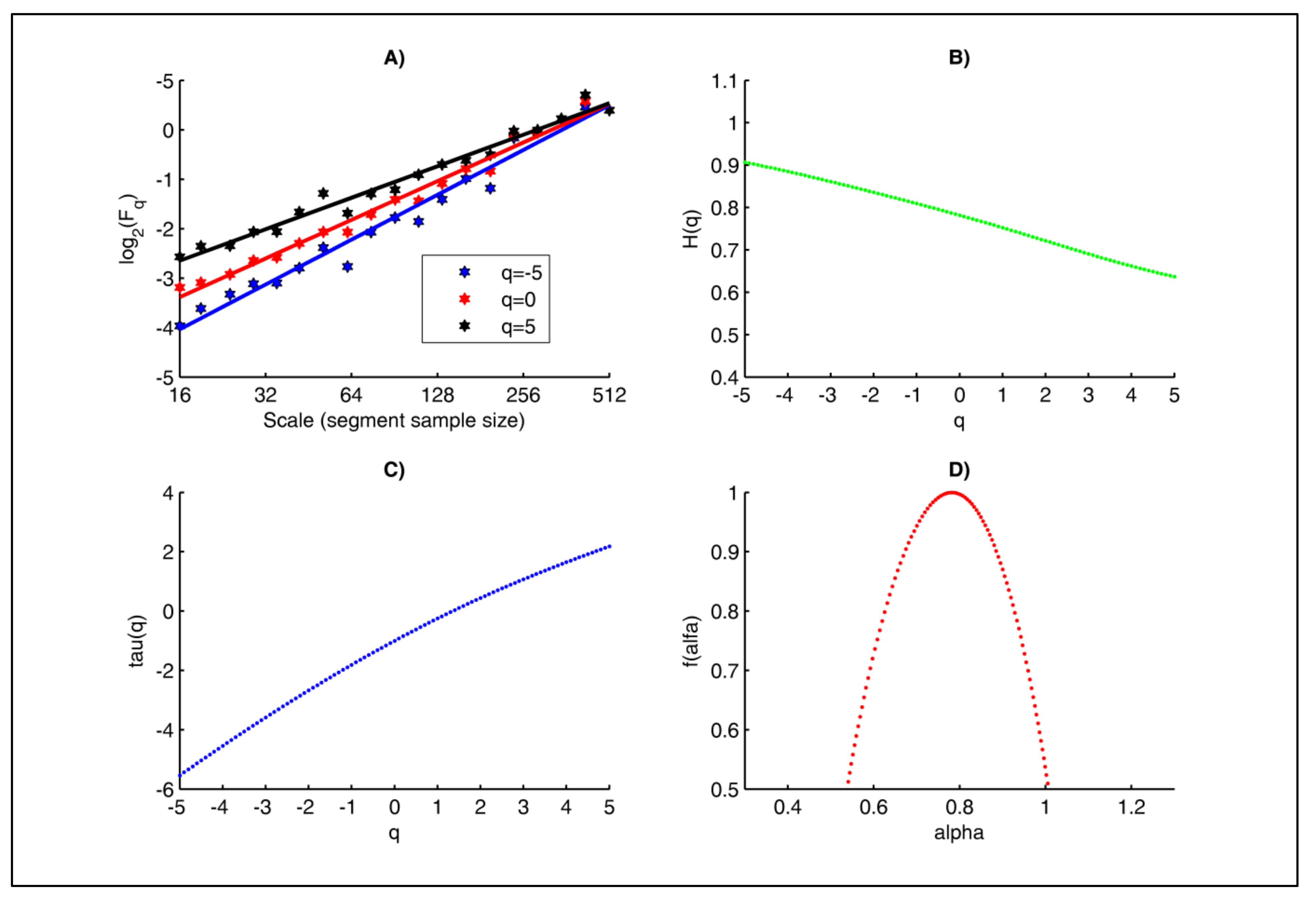
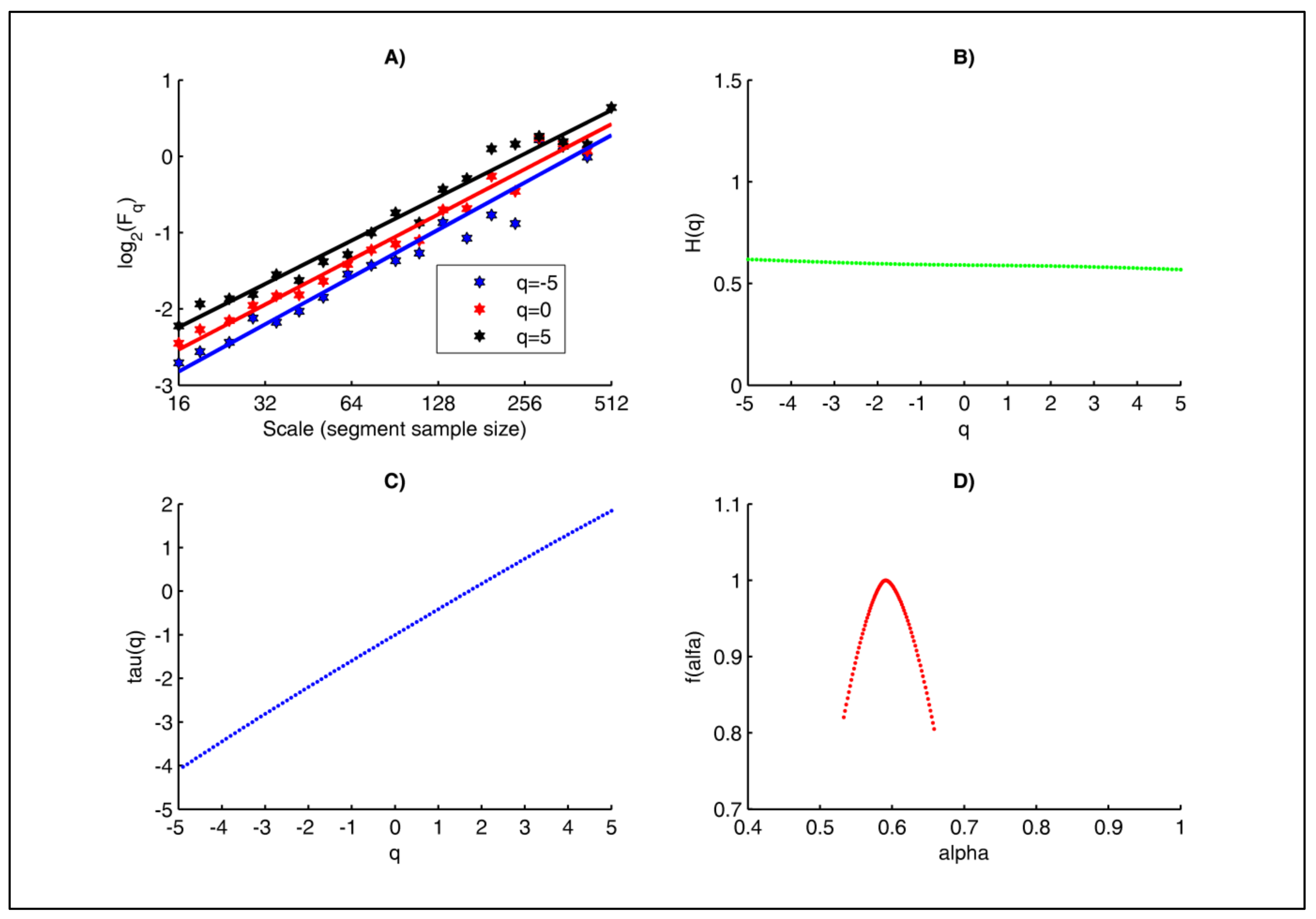
• The graphs of the Fq(scale) function for different values of the parameter q shown in Figure 6A and Figure 7A are for a healthy subject and an unhealthy subject (arrhythmia patient). The graphs for both subjects are straight lines, i.e., the studied RR time series are scale-invariant and therefore exhibit fractal behavior. The slopes of the Fq vs. q corresponding to a healthy individual are different, which is evidence of multifractal behavior of the studied cardiac signal. The graphs for the unhealthy subject are parallel, i.e., the slope of the oscillation functions is constant, and this observation can be interpreted as monofractal behavior;
• Figure 6B and Figure 7B show the dependence of the generalized Hurst exponent H(q) versus q for the RR time intervals of healthy and unhealthy subjects. The range of values of the Hurst exponent for a healthy subject varies from 0.9 to 0.6 in the case of different values of the q parameter. Therefore, the RR intervals for healthy subjects have a multifractal behavior. In the case of an unhealthy subject (arrhythmia patient), the Hurst exponent is a constant at different values of the q parameters; therefore, the investigated signal has a monofractal behavior. From the graph in Figure 6B, for the healthy patient it can be seen that H(q = 2) = 0.7848, and for the diseased patient (Figure 6B) H(q = 2) = 0.5912. In Table 1 are shown the values of this parameter for the two studied groups. This parameter has statistical significance (p < 0.05), and the determined AUC value is 0.789;
• Figure 6C and Figure 7C show the tau(q) curves of healthy and unhealthy subjects. When the function tau(q) is a convex curve, this is evidence that the studied signal has a multifractal behavior. In the case where tau(q) is a straight line, this is evidence that the signal is monofractal. Therefore, the RR time intervals of the healthy subjects have a multifractal behavior, while the signals of the patients with arrhythmia are monofractals;
• The graphs on Figure 6D and Figure 7D illustrate the multifractal spectrum of RR intervals for healthy and unhealthy individuals. The multifractal spectrum of the RR intervals of the healthy subject (Figure 6D) is Δα = α_max − α_min = 1.0077 − 0.5224 = 0.4853, while for the unhealthy subject (Figure 6D) it is Δα = α_max − α_min =0.6580 − 0.5329 = 0.1251. The signal of the healthy subject has a broad multifractal spectrum, while the signal of the unhealthy subject (arrhythmia patient) has a narrow multifractal spectrum that is about 4 times smaller than that of the healthy subject. The graph in Figure 7D corresponding to the arrhythmia patient is an example of a monofractal process. In Table 1 are shown the values of the multifractal spectrum of the two studied groups. The value of this parameter is higher in healthy individuals, which is due to the higher HRV. This parameter has statistical significance (p < 0.05), and the determined value of AUC (Figure 8) is 0.798.

Based on the results obtained for the determined AUC values for the parameters H(q = 2) and the multifractal spectrum F(α), it follows that MFDFA is a method with a good diagnostic evaluation and can be used to distinguish sick from healthy individuals.

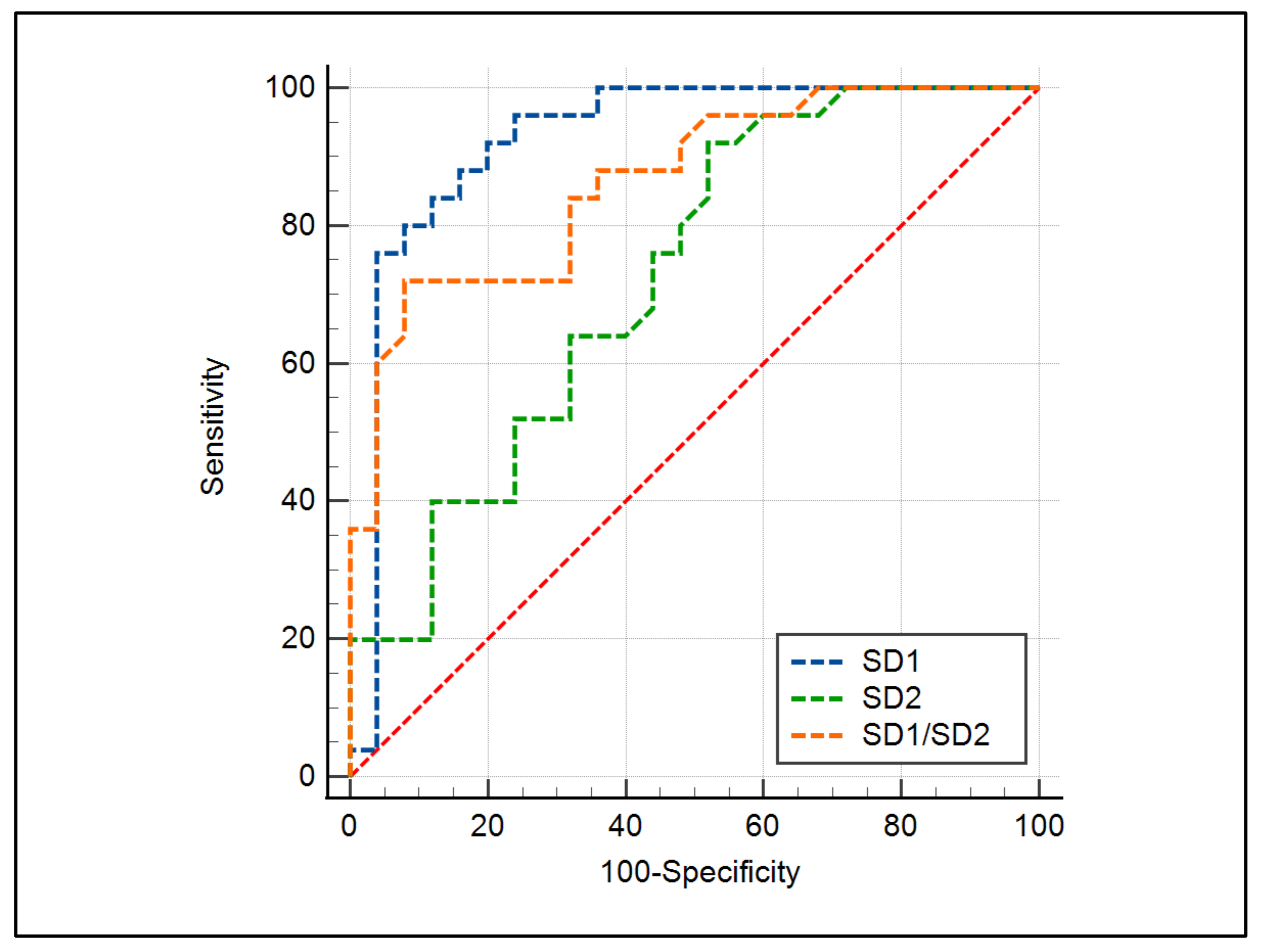
3.2. Evaluation of the Poincaré Plot

The visual analysis of HRV based on the Poincaré diagram provides information about the health status of the study subjects. The graphs constructed from the Poincaré plot for a healthy individual and arrhythmia patients are shown in Figure 8A,B. The graph of a healthy individual has the shape of a comet with a pointed lower part and gradually widening towards the top. The graph of the arrhythmia patient is fan-shaped.

In healthy individuals, the shape of the ellipse is clearly defined, while in patients with arrhythmia (or other diseases), the length and width of the ellipse may be approximately equal, and the ellipse may approach a circle. In Table 1 are shown the results of the studied parameters SD₁, SD₂, SD₁/SD₂ as mean ± std.

To differentiate the two studied groups, the statistical significance (p-value) was determined by t-test. The obtained results show that the p-value is less than 0.05 for the studied parameters; therefore, with this method, the two groups can be distinguished. Figure 9 shows the ROC curves for the studied parameters, and the determined AUC values are shown in Table 1. Based on the determined AUC values, the results obtained for the diagnostic evaluation of the parameters are as follows:

• SD₁ = 0.925—the parameter has an excellent diagnostic value;
• SD₂ = 0.725—the parameter has a good diagnostic value;
• SD₁/SD₂ = 0.863—the parameter has a very good diagnostic value.

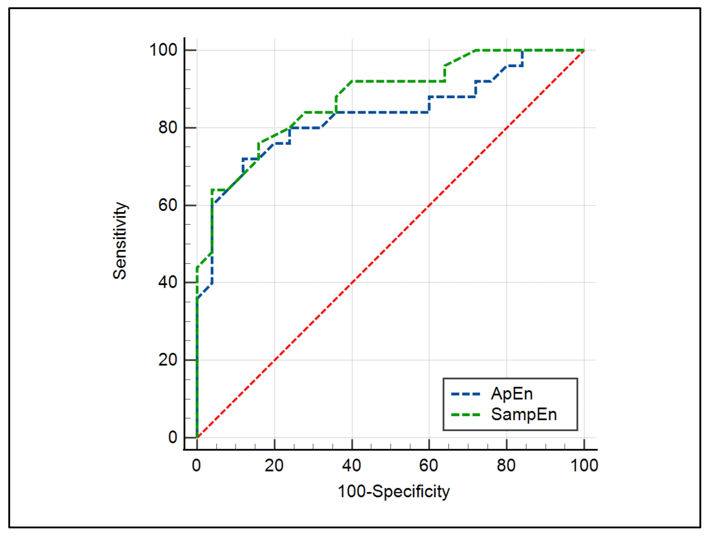
3.3. Evaluation of the ApEn and SampEn Methods

The ApEn and SampEn methods can be used to study the dynamics of cardiac data consisting of the intervals between heartbeats. To determine ApEn and SampEn, it is necessary to set values for the parameters: m(subseries length) and r(tolerance). In our previous article [50], the following values were found to be appropriate: m = 2, r = 0.2. In Table 1 are shown the results of the determined values of the two entropies as mean ± std. The ROC curves for the studied parameters are presented in Figure 10. Based on the obtained results, the following conclusions can be drawn:

• The values of ApEn and SampEn were higher for the healthy subjects compared to those of the diseased subjects; therefore, the RR intervals of healthy subjects had greater complexity;
• For the two studied parameters ApEn and SampEn, the p-value is less than 0.05; therefore, these parameters have statistical significance, which makes it possible to distinguish between the two investigated groups;
• From the determined AUC values for ApEn and SampEn, it follows that a very good diagnostic score is obtained with these two methods.

4. Conclusions

This article presents the results of the application of nonlinear mathematical methods for the analysis of two groups of people: 25 healthy subjects (15 men, 10 women, mean age: 56.3 years) and 25 patients with arrhythmia (13 men, 12 women, mean age: 58.7 years). The obtained results are part of the scientific research carried out under the project “Investigation of the application of new mathematical methods for the analysis of cardiac data”, financed by the “Scientific Research” Fund, Bulgaria. Currently, most cardiologists experience difficulties with the use of fractal, multifractal and informational methods for the analysis of ECG signals and the accurate interpretation of the obtained results. However, the analysis of the dynamics of RR interval series by the application of these methods with a view to distinguishing healthy subjects from diseased ones is an important and interesting topic. The informational properties of these methods and their application in the study of the fractal, multifractal and informational properties of the intervals between heartbeats of the studied groups of patients show high efficiency and open perspectives for their future use in the diagnosis and prediction of cardiovascular diseases. The application of the Poincaré plot for the analysis of HRV is an effective tool for visualizing the fluctuations of the RR interval series. From the results, detailed information on the physiological status of patients can be obtained, which facilitates healthcare professionals in making accurate diagnoses, especially in cases of large amounts of information when analysing 24, 48 or 72 h Holter data. From the evaluation of the used nonlinear methods for the analysis of HRV, it follows that they have from good to excellent diagnostic values and can be used to distinguish healthy subjects from those with arrhythmia.

References

1. Haque, M.; Tariq, M.; Hussain, T. Presence of Multifractality in High-Energy Nuclear Collisions. J. Mod. Phys. 2014, 5, 1889–1895. [Google Scholar] [CrossRef]
2. Rafique, M.; Javid, I.; Javed, L.K.; Jane, K.K.; Saeed, U.R.; Lal, H. Multifractal detrended fluctuation analysis of soil radon (222Rn) and thoron (220Rn) time series. J. Radioanal. Nucl. Chem. Vol. 2021, 328, 425–434. [Google Scholar] [CrossRef]
3. Miloş, L.R.; Haţiegan, C.; Miloş, M.C.; Barna, F.M.; Boțoc, C. Multifractal Detrended Fluctuation Analysis (MF-DFA) of Stock Market Indexes Empirical Evidence from Seven Central and Eastern European Markets. Sustainability 2020, 12, 535. [Google Scholar] [CrossRef]
4. Goldberger, A.L. Fractal variability versus pathologic periodicity: Complexity loss and stereotypy in disease. Perspect. Biol. Med. 1996, 4, 543–561. [Google Scholar] [CrossRef]
5. Das, N.; Chatterjee, S.; Kumar, S.; Pradhan, A.; Panigrahi, P.; Vitkin, I.A.; Ghosh, N. Tissue multifractality and Born approximation in analysis of light scattering: A novel approach for precancers detection. Sci. Rep. 2014, 20, 6129. [Google Scholar] [CrossRef]
6. Das, N.; Alexandrov, S.; Gilligan, K.E.; Dwyer, R.M.; Saager, R.B.; Ghosh, N.; Leahy, M. Characterization of nanosensitive multifractality in submicron scale tissue morphology and its alteration in tumor progression. J. Biomed. Opt. 2021, 26, 016003. [Google Scholar] [CrossRef]
7. Owis, M.I.; Abou-Zied, A.H.; Youssef, A.-B.M.; Kadah, Y.M. Study of features based on nonlinear dynamical modeling in ECG arrhythmia detection and classification. IEEE Trans. Biomed. Eng. 2002, 49, 733–736. [Google Scholar] [CrossRef]
8. Kumar, P.; Das, A.K.; Halder, S. Time-domain HRV Analysis of ECG Signal under Different Body Postures. Procedia Comput. Sci. 2020, 167, 1705–1710. [Google Scholar] [CrossRef]
9. Kumar, D.M.; Prasannakumar, S.C.; Sudarshan, B.G.; Jayadevappa, D. Heart Rate Variability Analysis: A Review. Int. J. Adv. Technol. Eng. Sci. 2013, 1, 9–24. [Google Scholar]
10. Costa, M.D.; Davis, R.B.; Goldberger, A.L. Heart rate fragmentation: A new approach to the analysis or cardiac interbeat internal dynamics. Front. Psychol 2017, 8, 255. [Google Scholar] [CrossRef]
11. Malik, M. Task Force of the European Society of Cardiology and the North American Society of Pacing and Electrophysiology, Heart rate variability—Standards of measurement, physiological interpretation, and clinical use. Circulation 1996, 93, 1043–1065. [Google Scholar] [CrossRef]
12. Eke, A.; Herman, P.; Kocsis, L.; Kozak, L.R. Fractal characterization of complexity in temporal physiological signals. Physiol. Meas. 2002, 23, R1–R38. [Google Scholar] [CrossRef] [PubMed]
13. Ivanov, P.; Amaral, L.; Goldberger, A.; Halvin, S.; Rosenblum, M.; Stanley, H.; Struzik, Z. From 1/f noise to multifractal cascades in heartbeat dynamics. Chaos 2001, 11, 641–652. [Google Scholar] [CrossRef] [PubMed]
14. Ivanov, P.; Chen, Z.; Hu, K.; Stanley, H. Multiscale aspects of cardiac control. Phys. A 2004, 344, 685–704. [Google Scholar] [CrossRef]
15. Ivanov, P.; Amaral, L.; Goldberger, A.; Halvin, S.; Rosenblum, M.; Stanley, H.; Struzik, Z. Multifractality in human heartbeat dynamics. Nature 1999, 399, 461–465. [Google Scholar] [CrossRef]
16. Acharya, U.R.; Suri, J.S.; Spaan, J.A.E.; Krishnan, A.M. Advances in Cardiac Signal Processing; Springer: Berlin/Heidelberg, Germany, 2007. [Google Scholar] [CrossRef]
17. Kleiger, R.; Miller, J.; Bigger, J.; Moss, A.J. Decreased Heart Rate Variability and It‘s Association with Increased Mortality After Acute Myocardial Infarction. Am. J. Cardiol. 1987, 59, 256–262. [Google Scholar] [CrossRef]
18. Glenny, R.W.; Robertson, H.T.; Yamashiro, S.; Bassingthwaighte, J.B. Applications of fractal analysis to physiology. J. Appl. Physiol. 1985, 70, 2351–2367. [Google Scholar] [CrossRef]
19. Haykin, S.; Li, X.B. Detection of signals in chaos. Proc. IEEE 1995, 83, 95–122. [Google Scholar] [CrossRef]
20. Kale, M.; Butar, F.B. Fractal analysis of Time Series and Distribution Properties of Hurst Exponent. J. Math. Sci. Math. Educ. 2011, 5, 8–19. [Google Scholar]
21. Kalisky, T.; Ashkenazy, Y.; Havlin, S. Volatility of fractal and multifractal time series. Isr. J. Earth Sci. 2007, 65, 47–56. [Google Scholar] [CrossRef]
22. Wang, J.; Ning, Y.; Chen, Y. Multifractal analysis of electronic cardiogram taken from healthy and unhealthy adult subjects. Phys. A 2003, 323, 561–568. [Google Scholar] [CrossRef]
23. Martinis, M.; Knežević, A.; Krstačić, G.; Vargović, E. Changes in the Hurst exponent of heart beat intervals during physical activities. Phys. Rev. E 2004, 70, 012903. [Google Scholar] [CrossRef] [PubMed]
24. Sheluhin, O.I.; Smolskiy, S.M.; Osin, A.V. Self-Similar Processes in Telecommunications; John Wiley & Sons, Ltd.: England, UK, 2006. [Google Scholar]
25. Biswas, A.; Zeleke, T.B.; Si, B.C. Multifractal detrended fluctuation analysis in examining scaling properties of the spatial patterns of soil water storage. Nonlinear Process Geophys. 2012, 19, 227–238. [Google Scholar] [CrossRef]
26. Delgado-Bonal, A.; Marshak, A. Approximate Entropy and Sample Entropy: A Comprehensive Tutorial. Entropy. Entropy 2019, 21, 541. [Google Scholar] [CrossRef]
27. Yentes, J.M.; Hunt, N.; Schmid, K.K.; Kaipust, J.P.; McGrath, D.; Stergiou, N. The Appropriate Use of Approximate Entropy and Sample Entropy with Short Data Sets. J. Artic. 2013, 44, e21060541. [Google Scholar] [CrossRef]
28. Tarvainen, M.P.; Lipponen, J.; Niskanen, J.P.; Ranta-Aho, P. Kubios HRV Version 3—User’s Guide. Kuopio: University of Eastern Finland 2016–2021. Available online: www.kubios.com (accessed on 3 November 2021).
29. Hurst, H.E.; Black, R.P.; Sinaika, Y.M. Long-Term Storage in Reservoirs: An Experimental Study; Constable: London, UK, 1965. [Google Scholar]
30. Nikolopoulos, D.; Moustris, K.; Petraki, E.; Koulougliotis, D.; Cantzos, D. Fractal and Long-Memory Traces in PM10 Time Series in Athens, Greece. Environments 2019, 6, 29. [Google Scholar] [CrossRef]
31. Brătian, V.; Acu, A.-M.; Oprean-Stan, C.; Dinga, E.; Ionescu, G.-M. Efficient or Fractal Market Hypothesis? A Stock Indexes Modelling Using Geometric Brownian Motion and Geometric Fractional Brownian Motion. Mathematics 2021, 9, 2983. [Google Scholar] [CrossRef]
32. Mielniczuk, J.; Wojdyllo, P. Estimation of Hurst exponent revisited. Comput. Stat. Data Anal. 2007, 51, 4510–4525. [Google Scholar] [CrossRef]
33. Naiman, E. The Hurst Index Calculation to Identify Persistence of the Financial Markets and Macroeconomic Indicators. Ukr. J. Ekon. 2009, 10, 18–28. [Google Scholar]
34. Peng, C.-K.; Buldyrev, S.V.; Havlin, S.; Simons, M.; Stanley, H.E.; Goldberger, A.L. Mosaic organization of dna nucleotides. Phys. Rev. E. Stat. Phys. Plasmas Fluids Relat. Interdiscip. Top. 1994, 49, 1685–1689. [Google Scholar] [CrossRef]
35. Peng, C.-K.; Havlin, S.; Stanley, H.E.; Goldberger, A.L. Quantification of scaling exponents and crossover phenomena in nonstationary heartbeat time series. Chaos 1995, 5, 82–87. [Google Scholar] [CrossRef] [PubMed]
36. Costa, N.; Silva, C.; Ferreira, P. Long-range behaviour and correlation in detrended fluctuation analysis and DCCA analysis of cryptocurrencies. Int. J. Financ. Stud. 2019, 7, 51. [Google Scholar] [CrossRef]
37. Golińska, A.K. Detrended Fluctuation Analysis (DFA) in Biomedical Signal Processing: Selected Examples. Stud. Log. Gramm. Rhetor. 2012, 29, 107–115. [Google Scholar]
38. Hardstone, R.; Poil, S.-S.; Schiavone, G.; Jansen, R.; Nikulin, V.V.; Mansvelder, H.D.; Linkenkaer-Hansen, K. Detrended Fluctuation Analysis: A Scale-Free View on Neuronal Oscillations. Front. Physiol. 2012, 3, 450. [Google Scholar] [CrossRef]
39. Maraun, D.; Rust, H.W.; Timmer, J. Tempting long-memory—On the interpretation of DFA results. Nonlinear Process. Geophys. Eur. Geosci. Union 2004, 11, 495–503. [Google Scholar] [CrossRef]
40. Kantelhardt, J.W.; Zschiegner, S.A.; Koscielny-Bunde, E.; Havlin, S.; Bunde, A.; Stanley, H.E. Multifractal detrended fluctuation analysis of nonstationary time series. Phys. A: Stat. Mech. Its Appl. 2002, 316, 87–114. [Google Scholar] [CrossRef]
41. Sassi, R.; Gabriella, M.S.; Cerutti, S. Multifractality and heart rate variability. Chaos 2009, 19, 028507. [Google Scholar] [CrossRef]
42. Li, E.; Mu, X.; Zhao, G.; Gao, P. Multifractal Detrended Fluctuation Analysis of Streamflow in the Yellow River Bain, China. Water 2015, 7, 1670–1686. [Google Scholar] [CrossRef]
43. Salat, H.; Murcio, R.; Arcaute, E. Multifractal methodology. Phys. A Stat. Mech. 2017, 473, 467–487. [Google Scholar] [CrossRef]
44. Ernst, G. Heart Rate Variability; Springer: London, UK, 2014. [Google Scholar] [CrossRef]
45. Byun, S.; Kim, A.Y.; Jang, E.H.; Kim, S.; Choi, K.W.; Yu, H.Y.; Jeon, H.J. Entropy analysis of heart rate variability and its application to recognize major depressive disorder: A pilot study. Technol. Health Care 2019, 27, 407–424. [Google Scholar] [CrossRef]
46. Montesinos, L.; Castaldo, R.; Pecchia, L. On the use of approximate entropy and sample entropy with centre of pressure time-series. J. Neuroeng. Rehabil 2018, 15, 116. [Google Scholar] [CrossRef] [PubMed]
47. Pincus, S.M. Approximate entropy as a measure of system complexity. Proc. Nati. Acad. Sci. USA 1991, 88, 2297–2301. [Google Scholar] [CrossRef] [PubMed]
48. Krupinski, E.A. Receiver Operating Characteristic (ROC) Analysis. Frontline Learn. Res. 2017, 5, 31–42. [Google Scholar] [CrossRef]
49. Salcedo-Martínez, A.; Zamora-Justo, J.A.; Muñoz-Diosdado, A. Analysis of the Hurst exponent in RR series of healthy subjects and congestive patients in a state of sleep and wakefulness and in healthy subjects in physical activity. AIP Conf. Proc. 2021, 2348, 040009. [Google Scholar] [CrossRef]
50. Gospodinova, E. Fractal time series analysis by using entropy and hurst exponent. In Proceedings of the 23rd International Conference on Computer Systems and Technologies, Ruse, Bulgaria, 17–18 June 2022; pp. 69–75. [Google Scholar] [CrossRef]
Figure 1. Poincaré plot graph of a healthy subject containing around 100,000 RR time intervals.
Fractalfract 07 00388 g001
Figure 2. Visual templates of the Poincaré plot depending on the shape of the points in the segment for a healthy subject and three unhealthy ones with various diseases. (A) The template of the Poincaré plot of the healthy subject has the shape of a comet. (B) The template of the Poincaré plot of the first unhealthy subject (syncope) has the shape of a torpedo. (C) The template of the Poincaré plot of the second unhealthy subject (arrhythmia) has the shape of a fan. (D) The template of the Poincaré plot of the third unhealthy subject (heart failure) has a complex shape.
Fractalfract 07 00388 g002
Figure 3. R/S statistics plots for the RR time intervals for a healthy subject (A) and for an arrhythmia patient (B). HRV analysis results of healthy and unhealthy subjects using the R/S method to determine the Hurst exponent value. The value of this parameter is determined by constructing a linear regression model between the variables Log10(R/S) and Log10(m). (A) For the healthy subject, the obtained value of the Hurst exponent is H = 0.956. (B) For the unhealthy subject (arrhythmia), this parameter value is H = 0.681, and it is lower than the value of the healthy subject.
Fractalfract 07 00388 g003
Figure 4. HRV analysis results of healthy and unhealthy subjects where the DFA method is used to determine the exponents: α1, α2 and αall. The cardiac signal is divided into segments, and the dependence between Log10(Fs) and Log10(s) is determined for each one of them. The linear behaviour of the function F(s) indicates the presence of self-similarity (fractality) for the studied signals, which are displayed on the figure. Panel (A) corresponds to the healthy subject, with the values of the parameters α1, α2 and αall determined by the slopes of the lines (green, red, blue). These slopes are greater compared to the slopes of the lines for the unhealthy subject (arrhythmia), which are shown on panel (B).
Fractalfract 07 00388 g004
Figure 5. ROC curves for the parameters of the R/S, DFA and MFDFA methods.
Fractalfract 07 00388 g005
Figure 6. HRV analysis results of the healthy subject using the MFDFA method. (A) The scaling function Fq (dots) and the corresponding regression slopes (lines) for three different values of the parameter q: −5, 0, 5 are shown; the regression lines are not parallel, which is evidence that the cardiac signal (RR time series) is multifractal. (B) The plot of the generalized Hurst exponent H(q) vs. parameter q indicates that the signal is multifractal, because H(q) is dependent on q. (C) The plot of the multifractal scaling exponent tau(q) exhibits a nonlinear dependence for q > 0, indicating again that the signal is multifractal. (D) The multifractal spectrum F(alpha) vs. parameter alpha for the healthy subject is wider compared to the unhealthy subject.
Fractalfract 07 00388 g006
Figure 7. HRV analysis results of the unhealthy subject (arrhythmia patient) using the MFDFA method. (A) The scaling function Fq (dots) and the corresponding regression slopes (lines) for the following values of parameter q: −5, 0, 5 are shown; the regression lines are parallel, which is evidence that the cardiac signal is monofractal. (B) The plot of the generalized Hurst exponent H(q) vs. parameter q indicates that the signal is monofractal, because the relationship between H(q) and q is constant. (C) The plot of the scaling exponent tau(q) exhibits a linear dependence for all q, indicating that the signal is monofractal. (D) The multifractal spectrum F(alpha) vs. parameter alpha for the unhealthy subject is narrower compared to the healthy subject.
Fractalfract 07 00388 g007
Figure 8. Poincaré plot graph for healthy and unhealthy subjects. (A) The template of the Poincaré plot of the healthy subject has the shape of a comet. (B) The template of the Poincaré plot of the unhealthy subject with arrhythmia has the shape of a fan.
Fractalfract 07 00388 g008
Figure 9. ROC curves for the parameters of the Poincaré plot.
Fractalfract 07 00388 g009
Figure 10. ROC curves for ApEn and SampEn.
Fractalfract 07 00388 g010