P-Bifurcation Analysis for a Fractional Damping Stochastic Nonlinear Equation with Gaussian White Noise

Abstract

This work aims to address the P-bifurcation of a stochastic nonlinear system with fractional damping driven by Gaussian white noise. Based on a stochastic averaging method, a fractional damping stochastic nonlinear equation has been studied. Furthermore, the expressions of drift and diffusion coefficients of the Fokker–Planck equation (FPKE) have been obtained. The probability density function (PDF), the steady solution of FPKE, has also been derived. Then, PDFs of two fractional damping Morse oscillators have been obtained. One can note that the analytical results coincide with the results of numerical simulation. Importantly, stochastic P-bifurcation of a fractional damping stochastic nonlinear Morse oscillator has been further addressed and analyzed.

1. Introduction and Background

Fractional calculus (FC) has proven to have a wide range of applications. As early as early the days of the establishment of integral calculus, some mathematicians began to consider the significance of FC, including Fourier, Abel, Riemann and Liouville, who made many contributions to the FC theory and formed a relatively complete FC definition [1,2,3,4,5].

With long-term unremitting efforts, FC theory has been established to a certain extent. Unfortunately, for a long time, FC was only a pure theoretical problem in the field of mathematics. Until recent decades, many scholars were surprised to find that the fractional order model is more suitable than the integer order model in solving some problems. Since then, fractional order models have been widely used in many fields [6,7,8,9,10,11].

In the natural, engineering and social fields, there are inevitable random excitations, such as atmospheric turbulence, ocean waves, earthquakes, jet noise and fluctuations of biological groups. The stochastic dynamics of systems with fractional derivatives attract many scholars to study them. There have been some effective methods to study the equations of nonlinear dynamic systems expressed by fractional differential equations, such as stochastic averaging method [12], path integral method [13], eigenvector expansion method [14], multi-scale method [15,16], Laplace transform [17], and Fourier transform [18,19]. These methods are of great significance to the study of nonlinear dynamic systems.

Stochastic analysis draws great attention due to its application in quantum physics, statistical physics, hydrodynamics, biology, economics, and mechanics [20]. The results obtained by applying the method of stochastic averaging to random vibration problems are discussed in [21]. The response and stability for a single-degree-of-freedom stochastic system has been studied by the stochastic averaging method [22]. The analytical solution of fractional nonlinear system has been addressed in [23]. As a unique nonlinear complex phenomenon in the field of dynamic systems, stochastic bifurcation is dedicated to evaluating the qualitative change of system response when the critical parameters change within a given time interval. Therefore, the study of stochastic bifurcation is helpful to understand the current state of system response and judge its change direction or range [24]. At present, there are two kinds of research methods to analyze stochastic bifurcation: one is to determine stochastic bifurcation by studying the change of the curve shape of probability density function, which is called phenomenological bifurcation (P-bifurcation); and the second is to determine the stochastic bifurcation of the system through the variation of the maximum Lyapunov exponent sign. That is called dynamic bifurcation (D-bifurcation).

In recent decades, stochastic bifurcation has been extensively used in engineering, physics, chemistry, economics, biology and other fields, and many achievements have been made so far. In 1984, Horsthemke and Lefever [25] published the first monograph on stochastic bifurcation. Zhu [26] studied stochastic Hopf bifurcation of a quasi-nonintegrable-Hamiltonian system using the stochastic averaging method. Yang [27] addressed P-bifurcation of a fractional-order vibration energy harvester under colored noise excitation. Schenk-Hoppé [28,29] investigated Hopf bifurcation based on the theory of stochastic dynamics together with a numerical method. Using the stochastic averaging and Khasminskii’s procedures, Zhu [30] investigated linear and nonlinear stochastic systems.

In the research of stochastic dynamic behavior, most of it is based on a Duffing oscillator. Based on the original van del Pol–Duffing oscillator mathematical model, this article introduces the Morse potential energy function instead of the original Duffing oscillator potential model to explore the stochastic P-bifurcation behavior of the Morse oscillator.

One knows that the Morse oscillator is widely used to describe the diatomic molecule in an electromagnetic field [31,32]. For instance, the motions of polyatomic molecules or diatomic molecules under an infrared laser environment can be modeled by the Morse oscillator [31,32]. Recently, fisher information [33] and vibrational resonance [34] of Morse oscillators have been investigated. The main difference between a Morse oscillator and harmonic oscillator is that it describes the non-bonding state, and the introduction of Morse potential energy can more accurately describe the molecular vibration.

In the present paper, based on the original mathematical model of the harmonic oscillator, the Morse potential energy function is introduced to replace the original simple harmonic oscillator potential model, and with the procedure of stochastic averaging, the approximation solution of a class fractional damping stochastic nonlinear equation governed by a general potential will be studied. Furthermore, the PDFs of two fractional damping stochastic Morse oscillators will be addressed in detail. Moreover, stochastic P-bifurcation of will also be discussed.

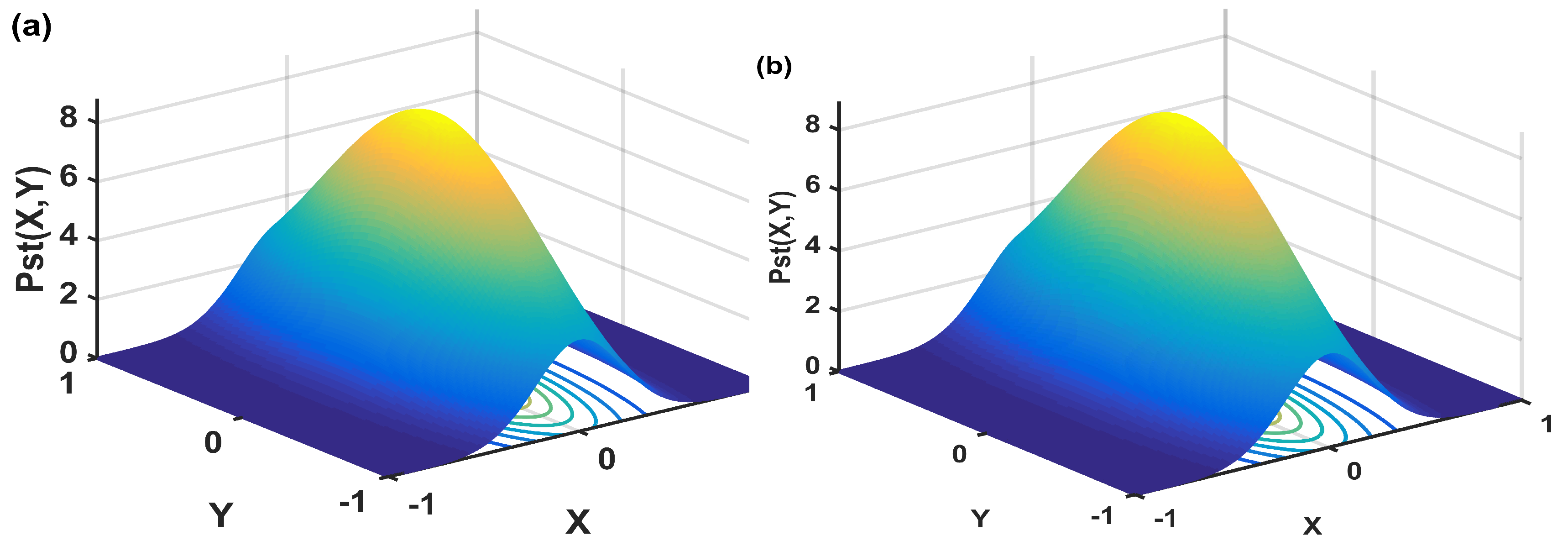
2. PDF for a Class Fractional Damping Stochastic Nonlinear Equation

One knows that mechanics models can be established by fractional differential equation due to viscoelastic bodies described by power-law kernels [35]. Additionally, the Hamiltonian system is often immersed in weak noise. Thus, a nonlinear conservative oscillator with small scale fractional derivative damping driven by white noise can be given by

$$\ddot{X}\left(t\right)+\epsilon c_1{D}_C^{\alpha }X\left(t\right)+\epsilon c_{2}h(X,\dot{X})+g\left(X\right)=W\left(t\right),0<\alpha <1,$$

(1)

in which $\epsilon$ presents a small positive constant. $c_1,c_2$ are two constant coefficients. $g\left(X\right)$ stands for a nonlinear continuous function of X. $h(X,\dot{X})$ denotes a continuous function of X and $\dot{X}$. $W\left(t\right)$ presents a Gaussian white noise, which meets

$$E\left[W\right(t\left)W\right(t+\tau \left)\right]=2D\delta \left(\tau \right).$$

(2)

$D_C^{\alpha }X\left(t\right)$ in Equation (1) indicates the Caputo fractional derivative defined by

$$D_C^{\alpha }X\left(t\right)=\frac{1}{\Gamma (1-\alpha )}\underset{0}{\overset{t}{\int }}\frac{\dot{X}\left(\mu \right)}{{(t-\mu )}^{\alpha }}\mathrm{d}\mu ,$$

(3)

in which $\Gamma (·)$ denotes a gamma function. It should be noted that $D_C^{\alpha }X\left(t\right)$ in Equation (1) can be modeled as a damping force [36] and Stokes force [35].

In the absence of damping and forcing, the potential is given by

$$V\left(X\right)=\underset{0}{\overset{X}{\int }}g\left(\mu \right)\mathrm{d}\mu .$$

(4)

Based on the procedure of stochastic averaging [26,27,28,29,30], one can take the following procedures:

$$X=X\left(t\right)=Acos\Theta \left(t\right),$$

(5)

$$Y=\dot{X}\left(t\right)=-A\omega sin\Theta \left(t\right),$$

(6)

$$\begin{array}{cc}\hfill & \Theta \left(t\right)=\omega t+\Psi \left(t\right),\end{array}$$

(7)

in which A, $\Theta$ and $\Psi$ denote three random processes. $A\left(t\right)$ and $\Psi \left(t\right)$ indicate two slowly varying processes, while $\Theta \left(t\right)$ denotes a quickly varying process. Differentiating Equation (5) and equating the resulting equation to Equation (6), one could obtain

$$\dot{A}cos\Theta -\dot{\Psi }\mathrm{A}sin\Theta =0.$$

(8)

Differentiating Equation (6), using Equations (1), (5) and (6), one can also yield

$$\begin{array}{cc}\hfill & \dot{\Psi }\frac{g(Acos\Theta )}{\omega }+\dot{A}\frac{g\left(A\right)-g(Acos\Theta )cos\Theta }{A\omega sin\Theta }\hfill \\ \hfill & =\epsilon c_1{D}^{\alpha }(Acos\Theta )+\epsilon c_{2}h(Acos\Theta ,-A\omega sin\Theta )-W\left(t\right).\hfill \end{array}$$

(9)

Thus, $\dot{A}$ and $\dot{\Psi }$ could be solved by Equations (8) and (9). Then, one yields

$$\frac{\mathrm{d}A}{\mathrm{d}t}=F_{11}(A,\Theta )+F_{12}(A,\Theta )+G_1(A,\Theta )W\left(t\right),$$

(10)

$$\frac{\mathrm{d}\Psi }{\mathrm{d}t}=F_2(A,\Theta )+G_2(A,\Theta )W\left(t\right),$$

(11)

where

$$F_1=F_{11}+F_{12},$$

(12)

$$F_{11}=\frac{A\omega sin\Theta }{g\left(A\right)}{c}_1{D}_C^{\alpha }(Acos\Theta ),$$

(13)

$$F_{12}=\frac{A\omega sin\Theta }{g\left(A\right)}{c}_{2}h(Acos\Theta ,-A\omega sin\Theta ),$$

(14)

$$F_2=\frac{\omega cos\Theta }{g\left(A\right)}{c}_1{D}_C^{\alpha }(Acos\Theta )+\frac{\omega cos\Theta }{g\left(A\right)}{c}_{2}h(Acos\Theta ,-A\omega sin\Theta ),$$

(15)

$$G_1=-\frac{A\omega sin\Theta }{g\left(A\right)},G_2=-\frac{\omega cos\Theta }{g\left(A\right)}.$$

(16)

Using Stratonovich–Khasminskii theorem [37], the averaged $It\widehat{o}$ equation of $A\left(t\right)$ is written as

$$\mathrm{d}A=m\left(A\right)\mathrm{d}t+\sigma \left(A\right)\mathrm{d}B\left(t\right),$$

(17)

in which the drift coefficient and diffusion coefficient are given by

$$\begin{array}{ccc}\hfill & & m\left(A\right)=\epsilon {〈F_{11}+F_{12}+D\frac{\partial G_1}{\partial A}{G}_1+D\frac{\partial G_1}{\partial \Gamma }{G}_2〉}_{\Theta },\hfill \\ & & {\sigma }^2\left(A\right)=\epsilon {〈2D{G}_1^2〉}_{\Theta },\hfill \end{array}$$

(18)

where averaging operation, ${〈·〉}_{\Theta }$, is given by

$${〈·〉}_{\Theta }=\underset{T\to \infty }{lim}\frac{1}{T}\underset{0}{\overset{T}{\int }}〈·〉\mathrm{d}t=\frac{1}{2\pi }\underset{0}{\overset{2\pi }{\int }}〈·〉\mathrm{d}\Theta .$$

(19)

Because A and $\Psi$ vary slow with time, we can obtain

$$\Theta \left(\mu \right)=\Theta (t-s)=\Theta \left(t\right)-\omega s.$$

(20)

Using the definition of fractional calculus, the averaging term of Equation (18) could be derived by

$$\begin{array}{ccc}\hfill {〈F_{11}〉}_{\Theta }& =& {〈\frac{A\omega sin\Theta }{g\left(A\right)}{c}_1{D}_C^{\alpha }(Acos\Theta )〉}_{\Theta }\hfill \\ & =& \frac{c_1}{g\left(A\right)}\underset{T\to \infty }{lim}\frac{1}{T}\underset{0}{\overset{T}{\int }}{D}_C^{\alpha }(Acos\Theta )\times A\omega sin\Theta \mathrm{d}t\hfill \\ & =& \frac{c_1}{\Gamma (1-\alpha )g\left(A\right)}\underset{T\to \infty }{lim}\frac{1}{T}\underset{0}{\overset{T}{\int }}\left\{\right[\underset{0}{\overset{t}{\int }}\frac{\dot{X}\left(\mu \right)}{{(t-\mu )}^{\alpha }}\mathrm{d}\mu ]\times A\omega sin(\omega t+\Psi )\}\mathrm{d}t\hfill \\ & =& \frac{-c_1}{\Gamma (1-\alpha )g\left(A\right)}\underset{T\to \infty }{lim}\frac{1}{T}\underset{0}{\overset{T}{\int }}\left\{\right[\underset{0}{\overset{t}{\int }}\frac{A\omega sin(\omega t+\Psi -\omega s)}{s^{\alpha }}\mathrm{d}s]\times A\omega sin(\omega t+\Psi )\}\mathrm{d}t\hfill \\ & =& \frac{-{\mathrm{c}}_1{A}^2{\omega }^2}{\Gamma (1-\alpha )g\left(A\right)}\underset{T\to \infty }{lim}\frac{1}{T}\{\underset{0}{\overset{T}{\int }}\left\{\right[\underset{0}{\overset{t}{\int }}\frac{cos\left(\omega s\right)}{s^{\alpha }}\mathrm{d}s]\times {sin}^2(\omega t+\Psi )\}\mathrm{d}t\hfill \\ & & +\underset{0}{\overset{T}{\int }}\left\{\right[\underset{0}{\overset{t}{\int }}\frac{sin\left(\omega s\right)}{s^{\alpha }}\mathrm{d}s]\times cos(\omega t+\Psi )sin(\omega t+\Psi )\}\mathrm{d}t\}\triangleq M_1+M_2.\hfill \end{array}$$

(21)

The first term in Equation (21) can be obtained

$$\begin{array}{ccc}\hfill M_1& =& \frac{-c_1{A}^2{\omega }^2}{\Gamma (1-\alpha )g\left(A\right)}\underset{T\to \infty }{lim}\frac{1}{T}\underset{0}{\overset{T}{\int }}[\underset{0}{\overset{t}{\int }}\frac{cos\left(\omega s\right)}{s^{\alpha }}\mathrm{d}s]\mathrm{d}\left(\frac{2\omega t-sin2(\omega t+\Psi )}{4}\right)\hfill \\ & =& \frac{-c_1{A}^2{\omega }^2}{4\Gamma (1-\alpha )g\left(A\right)}[\underset{T\to \infty }{lim}\left(\frac{2\omega t-sin2(\omega t+\Psi )}{T}\right)(\underset{0}{\overset{t}{\int }}\frac{cos\left(\omega s\right)}{s^{\alpha }}\mathrm{d}s{\left)\right|}_0^T\hfill \\ & & +\underset{T\to \infty }{lim}\frac{1}{T}\underset{0}{\overset{T}{\int }}(\underset{0}{\overset{t}{\int }}\frac{2\omega t-sin2(\omega t+\Psi )}{t^{\alpha }}cos\left(\omega t\right)\left)\mathrm{d}t\right]\triangleq M_{11}+M_{12}.\hfill \end{array}$$

(22)

Before going on, the following two relations will be used,

$$\underset{T\to \infty }{lim}\underset{0}{\overset{T}{\int }}\frac{sin\left(\omega s\right)}{s^{\alpha }}\mathrm{d}s={\omega }^{\alpha -1}\Gamma (1-\alpha )cos\frac{\alpha \pi }{2},$$

(23)

$$\underset{T\to \infty }{lim}\underset{0}{\overset{T}{\int }}\frac{cos\left(\omega s\right)}{s^{\alpha }}\mathrm{d}s={\omega }^{\alpha -1}\Gamma (1-\alpha )sin\frac{\alpha \pi }{2}.$$

(24)

Substituting Equations (23) and (24) into Equation (22), one has

$$\begin{array}{ccc}\hfill M_{11}& =& \frac{-c_1{A}^2{\omega }^2}{4\Gamma (1-\alpha )g\left(A\right)}\underset{T\to \infty }{lim}[2{\omega }^{\alpha }\Gamma (1-\alpha )sin\frac{\alpha \pi }{2}-\frac{sin2(\omega t+\Psi ){\omega }^{\alpha -1}\Gamma (1-\alpha )sin\frac{\alpha \pi }{2}}{T}]\hfill \\ & =& \frac{-c_1{A}^2}{2\Gamma (1-\alpha )g\left(A\right)}{\omega }^{\alpha +1}\Gamma (1-\alpha )sin\frac{\alpha \pi }{2},\hfill \end{array}$$

(25)

$$\begin{array}{ccc}\hfill M_{12}& =& \frac{-c_1{A}^2{\omega }^2}{4\Gamma (1-\alpha )g\left(A\right)}\underset{T\to \infty }{lim}\frac{1}{T}\underset{0}{\overset{T}{\int }}\frac{2\omega t-sin2(\omega t+\Psi )}{t^{\alpha }}cos\left(\omega t\right)\mathrm{d}t\hfill \\ & =& \frac{-c_1{A}^2{\omega }^2}{4\Gamma (1-\alpha )g\left(A\right)}\underset{T\to \infty }{[lim}\frac{1}{T}\underset{0}{\overset{T}{\int }}\frac{2\omega tcos\left(\omega t\right)}{t^{\alpha }}\mathrm{d}t-\underset{T\to \infty }{lim}\frac{1}{T}\underset{0}{\overset{T}{\int }}\frac{sin2(\omega t+\Psi )}{t^{\alpha }}cos\left(\omega t\right)\mathrm{d}t]\hfill \\ & =& 0,\hfill \end{array}$$

(26)

$$\begin{array}{ccc}\hfill M_2& =& \frac{-c_1{A}^2{\omega }^2}{4g\left(A\right)\Gamma (1-\alpha )}\underset{T\to \infty }{lim}\frac{1}{T}\underset{0}{\overset{T}{\int }}\left\{\right[\underset{0}{\overset{t}{\int }}\frac{sin\left(\omega s\right)}{s^{\alpha }}\mathrm{d}s]cos(\omega t+\Psi )sin(\omega t+\Psi )\}\mathrm{d}t\hfill \\ & =& 0,\hfill \end{array}$$

(27)

Thus,

$${〈F_{11}〉}_{\Theta }=M_{11}+M_{12}+M_2=\frac{-c_1{A}^2}{2g\left(A\right)}{\omega }^{\alpha +1}sin\frac{\alpha \pi }{2}.$$

(28)

Therefore, the drift coefficient and diffusion coefficient in Equation (18) can be given by

$$\begin{array}{cc}\hfill m\left(A\right)& =\epsilon {〈F_{11}〉}_{\Theta }+\frac{\epsilon c_{2}A}{2\pi g\left(A\right)}\underset{0}{\overset{2\pi }{\int }}\omega sin\Theta h(Acos\Theta ,-A\omega sin\Theta )\mathrm{d}\Theta +\epsilon D{〈\frac{\partial G_1}{\partial A}{G}_1+\frac{\partial G_1}{\partial \Gamma }{G}_2〉}_{\Theta },\hfill \\ \hfill {\sigma }^2\left(A\right)& =\epsilon {〈2D{G}_1^2〉}_{\Theta }.\hfill \end{array}$$

(29)

FPKE associated with Equation (17) is given by

$$\frac{\partial p}{\partial t}=-\frac{\partial }{\partial A}\left[m\left(A\right)p\right]+\frac{1}{2}\frac{{\partial }^2}{\partial A^2}\left[{\sigma }^2\left(A\right)p\right].$$

(30)

The boundary conditions for Equation (30) are

$$\begin{array}{ccc}\hfill & & p=c,A=0;\hfill \\ & & P,\partial p/\partial A\to 0,A\to \infty .\hfill \end{array}$$

(31)

Considering the boundary conditions in Equation (31), one can follow the normalization condition,

$${\int }_0^{\infty }p\left(A\right)dA=1.$$

(32)

The stationary solution of Equation (30) is given by

$$p\left(A\right)=\frac{C}{{\sigma }^2\left(A\right)}exp[\underset{0}{\overset{A}{\int }}\frac{2m\left(u\right)}{{\sigma }^2\left(u\right)}\mathrm{d}u],$$

(33)

where C denotes a normalization constant given by

$$C={[{\int }_0^{\infty }(\frac{1}{{\sigma }^2\left(A\right)}exp[{\int }_0^A\frac{2m\left(\mu \right)}{{\sigma }^2\left(\mu \right)}\mathrm{d}\mu ])\mathrm{d}A]}^{-1}.$$

(34)

Thus, using Equation (33), the stationary PDF of Hamiltonian $H=V\left(A\right)$ can be given by

$$p\left(H\right)=p\left(A\right)\left|\frac{\mathrm{d}A}{\mathrm{d}H}\right|=\frac{p\left(A\right)}{g\left(A\right)}{|}_{A=V^{-1}\left(H\right)},$$

(35)

in which $V^{-1}$ means the inverse function of H. Thus, the joint stationary PDF of the displacement and velocity could be given by

$$p(x,y)=\frac{p\left(H\right)}{T\left(H\right)}{|}_{H=\frac{1}{2}{y}^2+V\left(x\right)},$$

(36)

where

$$T\left(H\right)=\frac{2\pi }{\omega \left(A\right)}{|}_{A=V^{-1}\left(H\right)}.$$

(37)

3. Two Fractional Order Stochastic Morse Oscillators

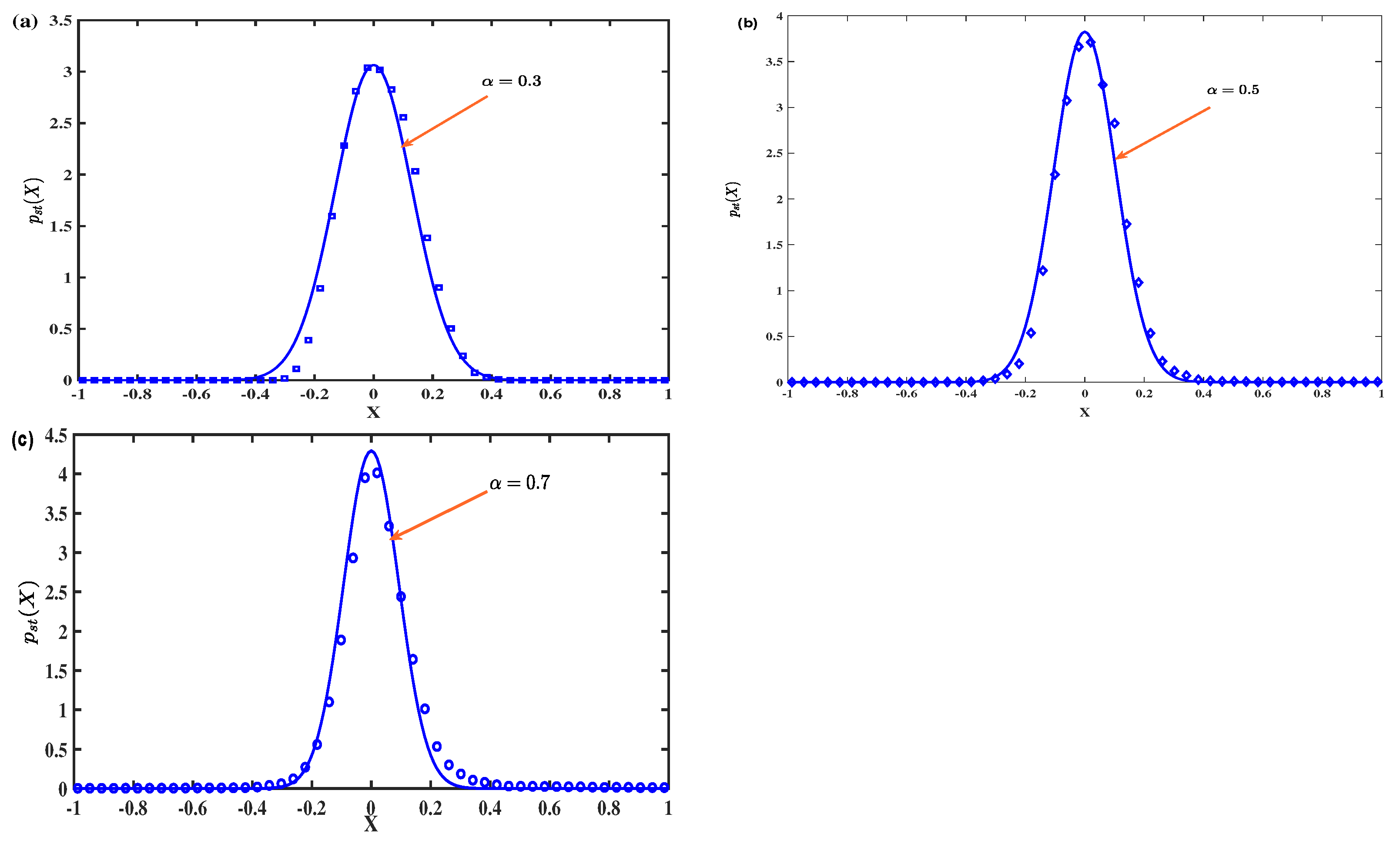
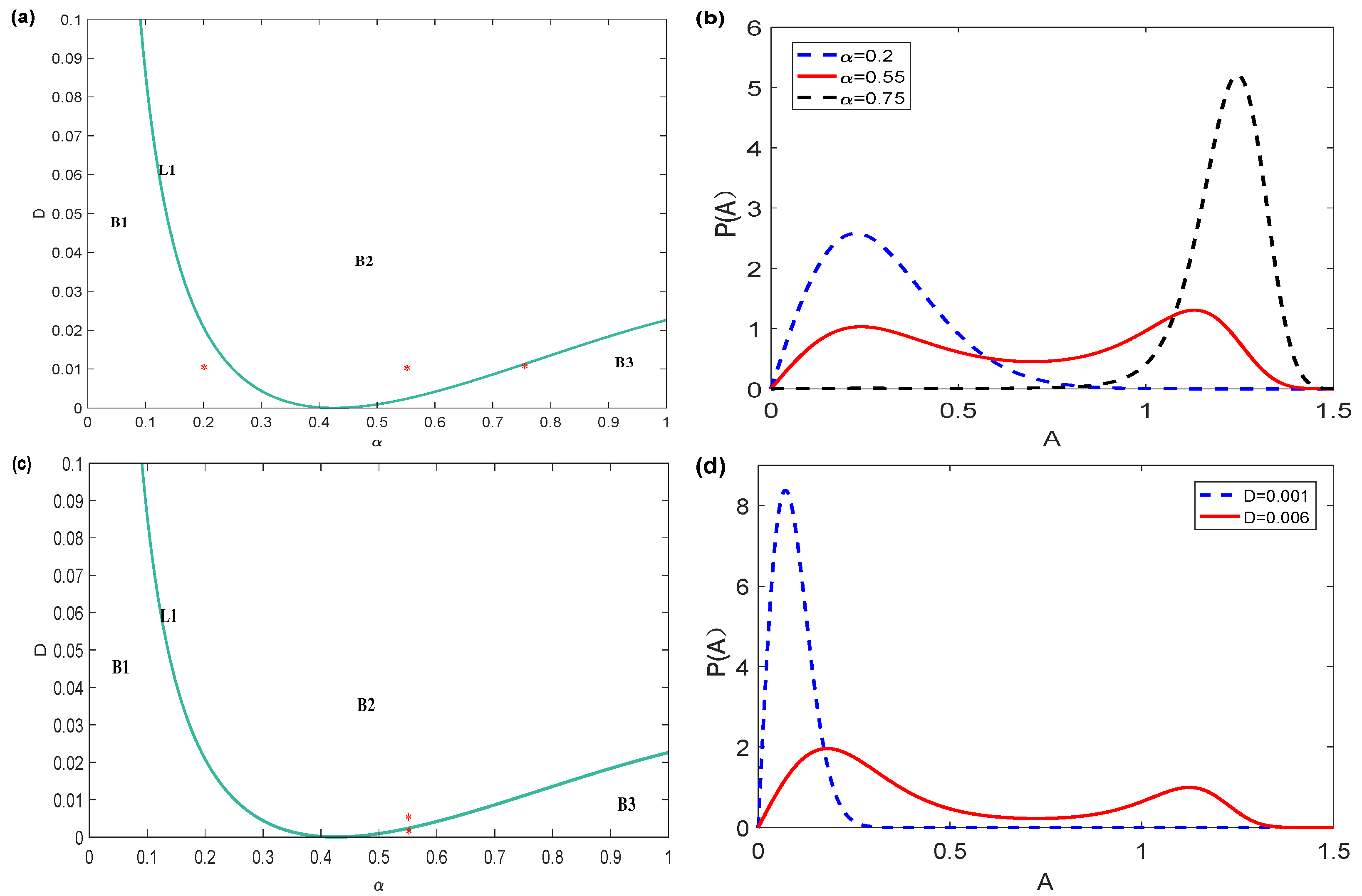
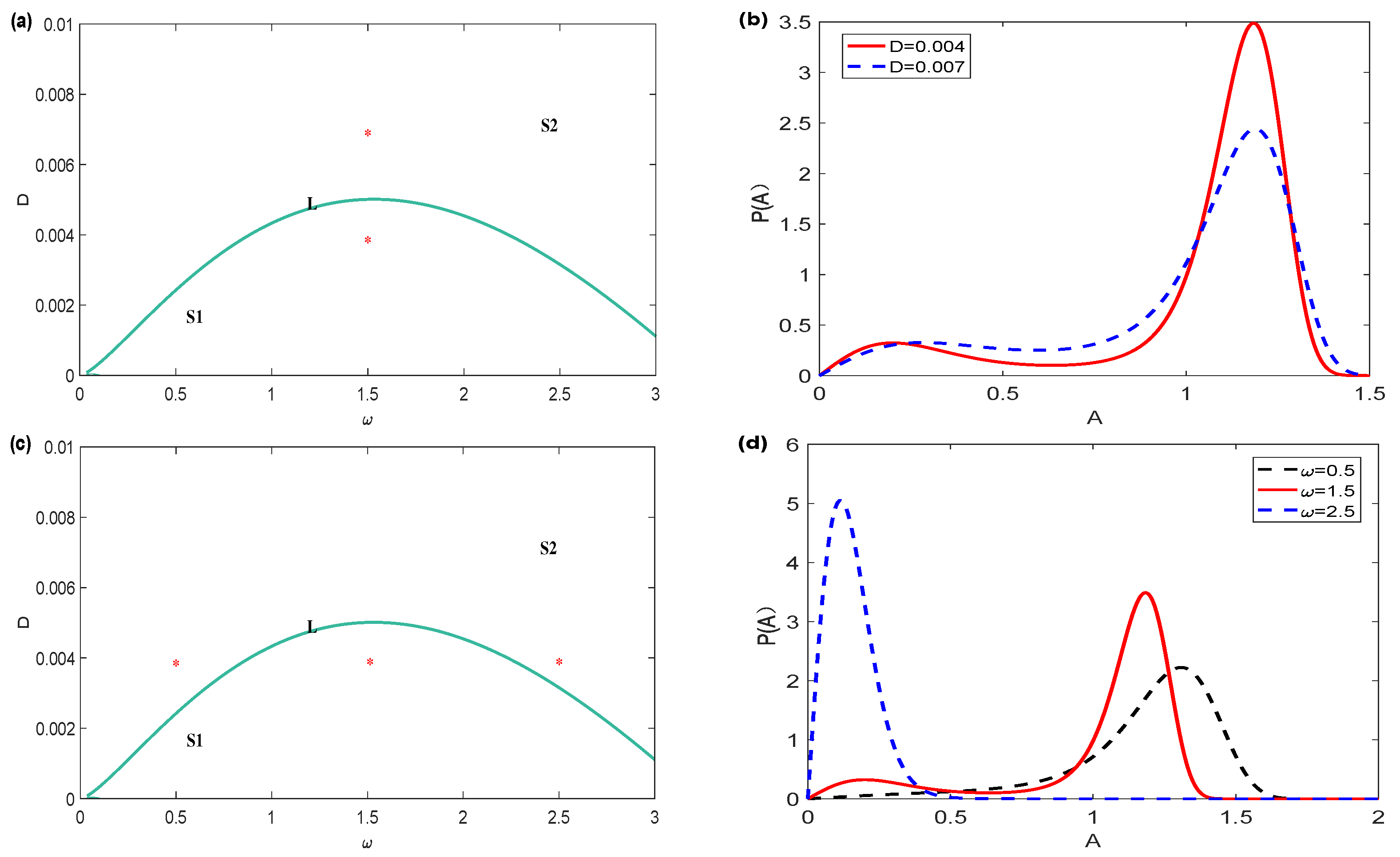
3.1. Fractional Order Stochastic Morse Oscillator with Constant Damping

In this subsection, we will consider a Caputo fractional damping stochastic Morse oscillator with Gaussian white noise given by

$$\ddot{X}\left(t\right)+b_1{D}_C^{\alpha }X\left(t\right)+b_{2}X\dot{X}+\beta (e^{-X}-e^{-2X})=W\left(t\right).$$

(38)

in which $W\left(t\right)$ presents a zero mean Gaussian white noise meeting Equation (2), $b_1$ denotes damping coefficient, $b_2$ and $\beta$ are constant coefficients. Based on the results in Section 2, the following transformations are adopted:

$$\begin{array}{cc}\hfill & X=X\left(t\right)=Acos\Phi \left(t\right),\hfill \\ \hfill & Y=\dot{X}\left(t\right)=-A\omega sin\Phi \left(t\right),\hfill \\ \hfill & \Phi \left(t\right)=\omega t+\Gamma ,\hfill \\ \hfill & V\left(X\right)=\frac{1}{2}\beta e^{-X}(e^{-X}-2).\hfill \end{array}$$

(39)

Using transformation (39), from Equation (38), one can follow two parts,

$$\frac{dA}{dt}=\epsilon F_{11}(A,\Theta )+\epsilon F_{12}(A,\Theta )+G_1(A,\Theta )W\left(t\right),$$

(40)

$$\frac{d\Gamma }{dt}=\epsilon F_2(A,\Theta )+G_2(A,\Theta )W\left(t\right).$$

(41)

where

$$\begin{array}{cc}\hfill h_{11}(A,\Gamma )& =\frac{b_1}{\omega }sin\Phi D_C^{\alpha }(Acos\Phi ),\hfill \\ \hfill h_{12}(A,\Gamma )& =-b_2{A}^2{sin}^2\Phi cos\Phi +\frac{\beta }{\omega }sin\Phi (e^{-Acos\Phi }-e^{-2Acos\Phi })-A\omega sin\Phi cos\Phi ,\hfill \\ \hfill h_{21}(A,\Gamma )& =-\frac{b_1}{\omega \mathrm{A}}cos\Phi D_C^{\alpha }(Acos\Phi ),\hfill \\ \hfill h_{22}(A,\Gamma )& =b_{2}A{cos}^2\Phi sin\Phi +\frac{\beta }{\omega \mathrm{A}}cos\Phi (e^{-Acos\Phi }-e^{-2Acos\Phi })-\omega {cos}^2\Phi ,\hfill \\ \hfill g_1(A,\Gamma )& =-\frac{sin\Phi }{\omega },g_2(A,\Gamma )=-\frac{cos\Phi }{\omega \mathrm{A}}.\hfill \end{array}$$

(42)

Utilizing the procedure in the Section 2, $It\widehat{o}$ differential Equation (17) with the drift coefficient and diffusion coefficient given by

$$\begin{array}{cc}\hfill & m\left(A\right)=-\frac{A{b}_1}{2}{\omega }^{\alpha -1}sin\frac{\alpha \pi }{2}+\frac{D}{2{\omega }^{2}A},\\ & {\sigma }^2\left(A\right)=\frac{D}{{\omega }^2}.\end{array}$$

(43)

Thus, stationary PDF of the system (38) could be given by

$$p\left(A\right)=\frac{b_{1}A{\omega }^{\alpha +1}sin\frac{\alpha \pi }{2}}{D}exp(-\frac{b_1{\omega }^{\alpha +1}sin\frac{\alpha \pi }{2}{A}^2}{2D}).$$

(44)

From Equations (33) and (35), the joint stationary PDF of X and Y could be written as

$$p_{st}(X,Y)=\frac{b_1{\omega }^{\alpha +2}sin\frac{\alpha \pi }{2}}{2\pi D}exp[-\frac{b_1{\omega }^{\alpha +1}sin\frac{\alpha \pi }{2}}{2D}(X^2+\frac{Y^2}{{\omega }^2})].$$

(45)

Correspondingly, stationary PDF of displacement and stationary PDF of velocity could be, respectively, obtained as follows:

$$p_{st}\left(X\right)=\frac{b_1{\omega }^{\alpha +3}\sqrt{\pi }sin\frac{\alpha \pi }{2}}{2\pi D\sqrt{\frac{b_1{\omega }^{\alpha +1}sin\frac{\alpha \pi }{2}}{2D}}}exp[-\frac{b_1{\omega }^{\alpha +1}sin\frac{\alpha \pi }{2}}{2D}{X}^2],$$

(46)

$$p_{st}\left(Y\right)=\frac{b_1{\omega }^{\alpha +2}\sqrt{\pi }sin\frac{\alpha \pi }{2}}{2\pi D\sqrt{\frac{b_1{\omega }^{\alpha +1}sin\frac{\alpha \pi }{2}}{2D}}}exp[-\frac{b_1{\omega }^{\alpha +1}sin\frac{\alpha \pi }{2}}{2{\omega }^{2}D}{Y}^2].$$

(47)

The stationary PDF versus displacement for a different fractional derivative order is plotted in Figure 1. To testify the precision of the analytical results, one can apply the stochastic Euler method (Equation (A1) in the Appendix A), and the results of Monte Carlo simulation for system (38) are also demonstrated in Figure 1.

It can be observed, from Figure 1, that the analytical results using the stochastic averaging procedure coincide with numerical simulation of a stochastic Morse oscillator (38). Meanwhile, it can be concluded that fractional order $\alpha$ greatly impacts PDF of stochastic Morse oscillator (38). Under the same noise intensity, the higher fractional order results in PDF lifting while the peak of PDF declines with the decline of fractional order $\alpha$. The stationary PDF versus displacement for different noise intensities D is plotted in Figure 2. One can figure out that the peak of PDF decreases with the rise of noise intensity D.

The stationary PDF versus amplitude for different $b_1$ is plotted in Figure 3. One can find that the peak of PDF lifts with the rising of $b_1$. Figure 4 displays the stationary PDF versus amplitude for different $\omega$. One can see that the peak of PDF lifts with the rising of $\omega$. Thus, both $b_1$ and $\omega$ can lift the response of PDF.

Figure 5 exhibits the stationary joint PDF of displacement and velocity, respectively, derived by using procedure of stochastic averaging and by using numerical simulation of system (49) with $\alpha =0.3$. It can be found out that the analysis results of PDF agree with the PDF of numerical simulation.

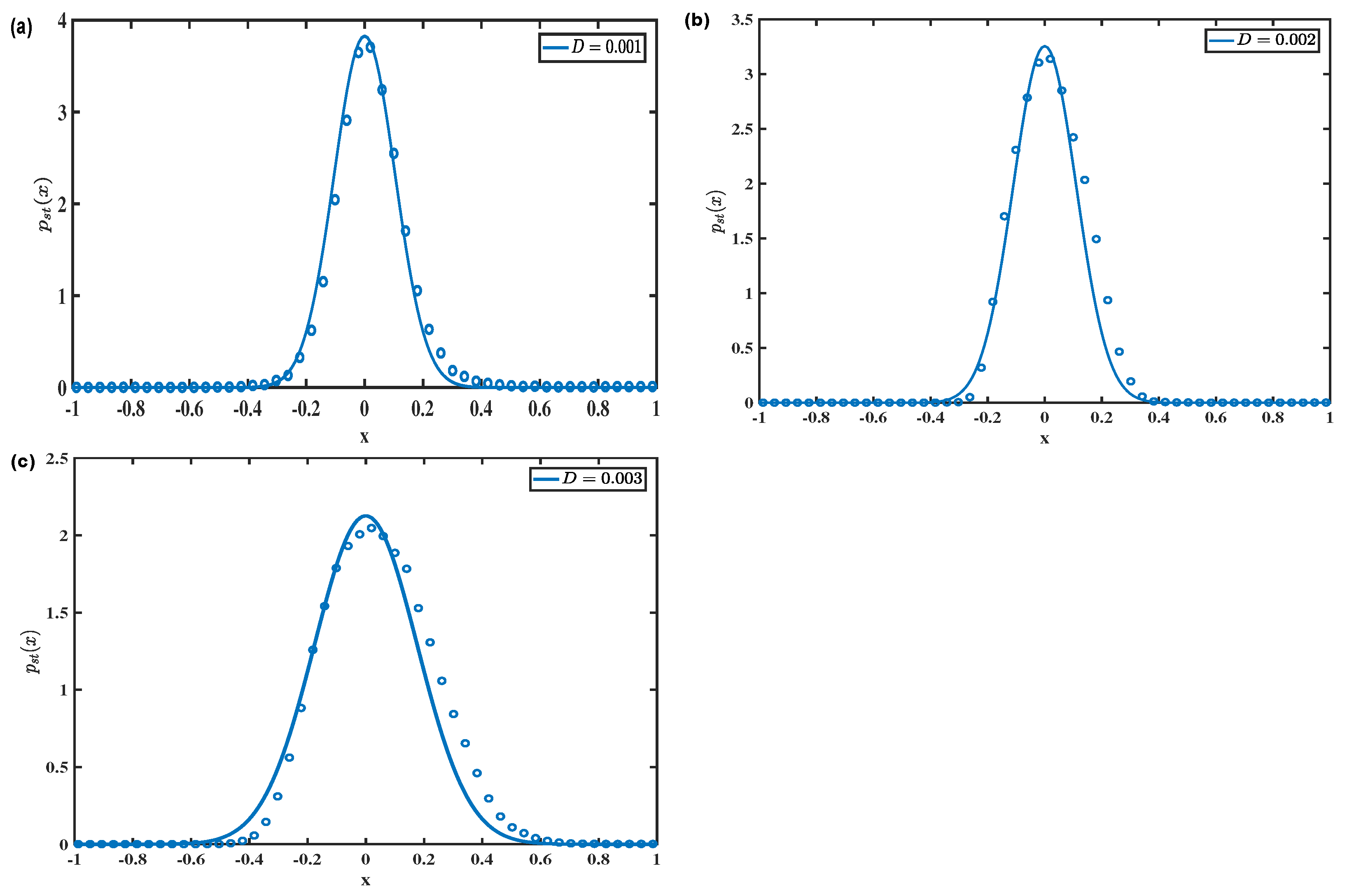
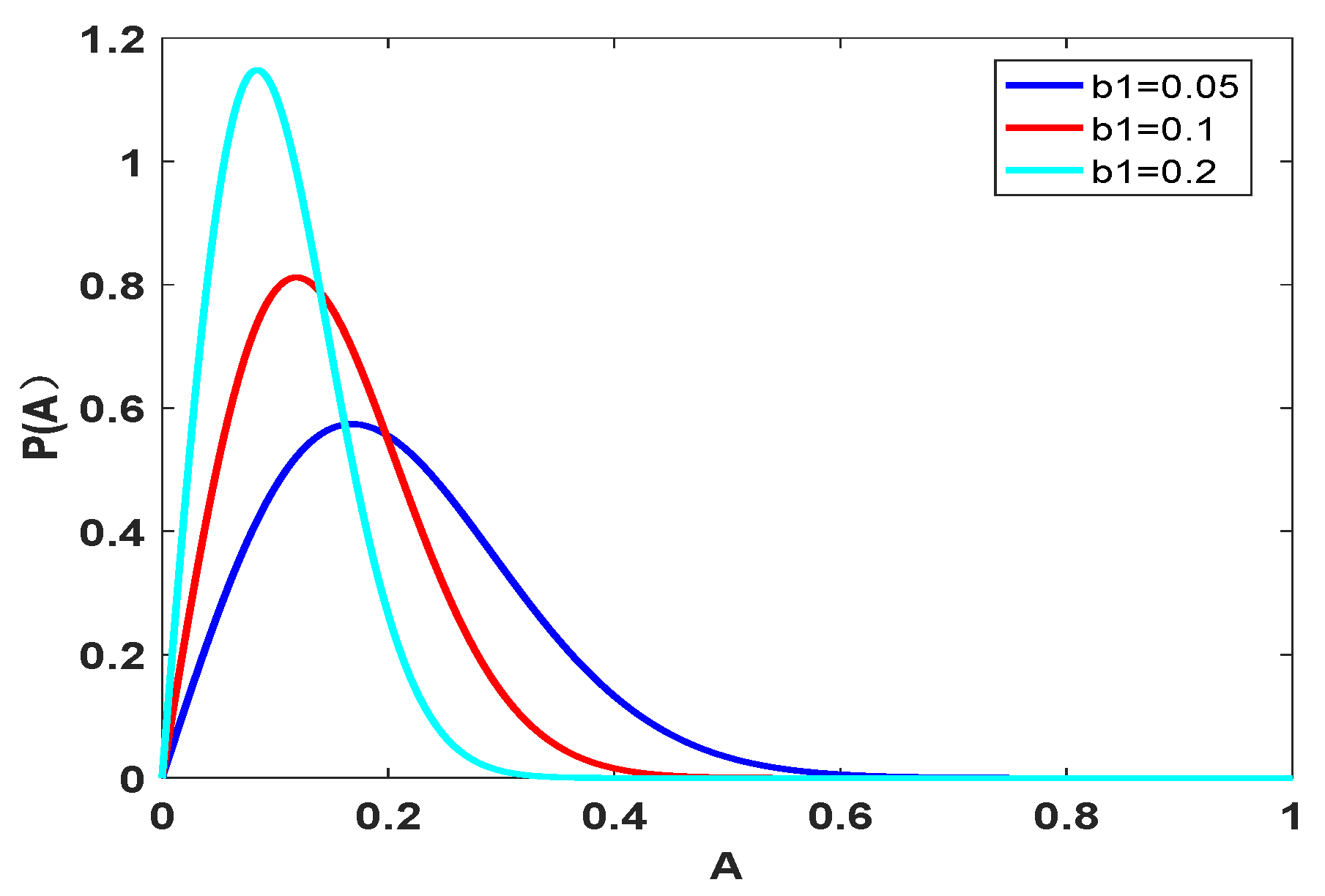
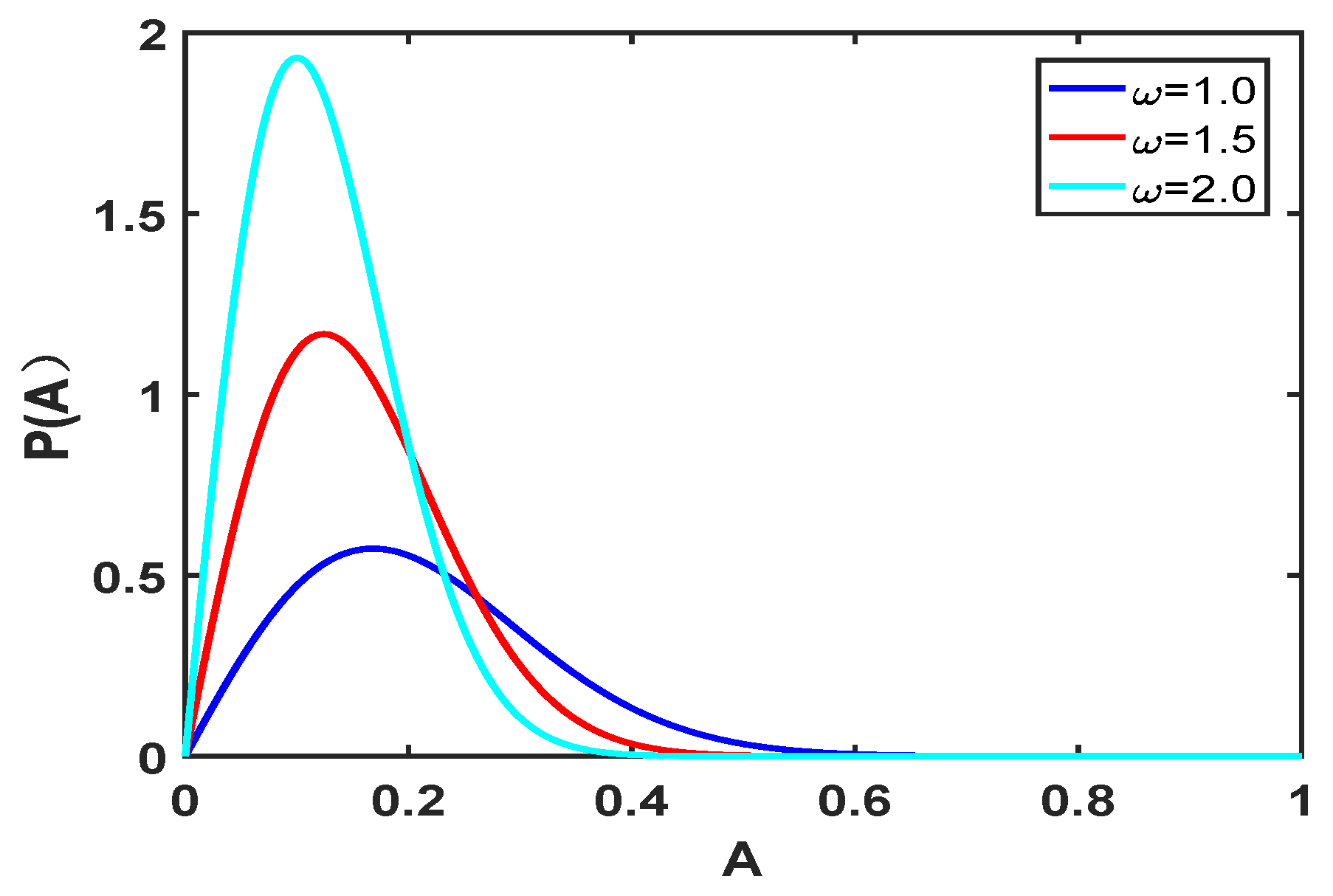
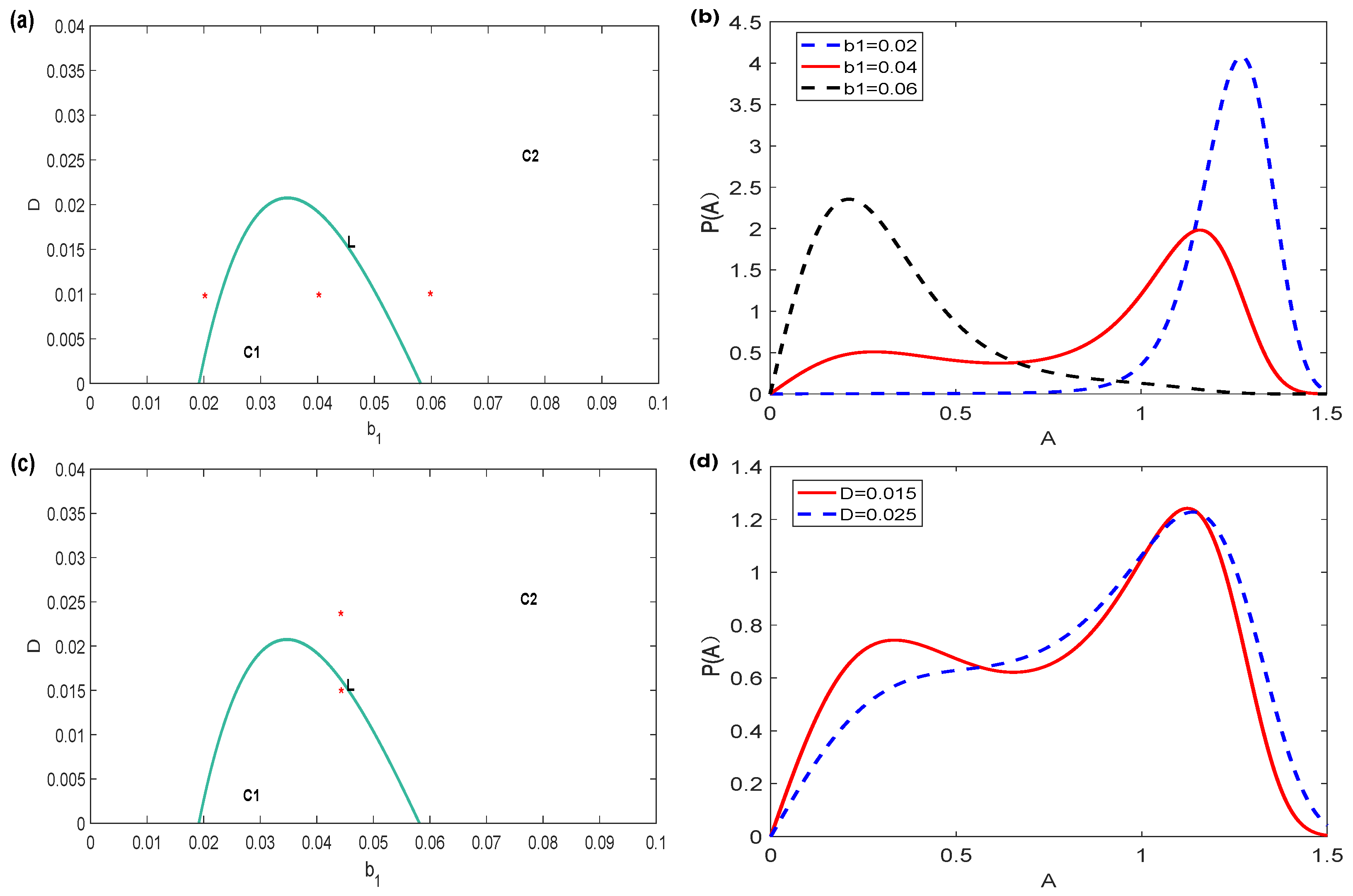
3.2. Fractional Order Stochastic Morse Oscillator with Nonlinear Damping

In this subsection, we will focus on a fractional order stochastic Morse oscillator with nonlinear damping subjected to a Gaussian white noise given by

$$\begin{array}{c}\hfill \ddot{X}+(a_1{X}^4-a_2{X}^2+a_0)D_C^{\alpha }X+(b_1+b_2{X}^2)\dot{X}+\beta (e^{-X}-e^{-2X})=W\left(t\right).\end{array}$$

(48)

in which $W\left(t\right)$ presents a zero mean Gaussian white noise meeting Equation (2). $a_1{X}^4-a_2{X}^2+a_0$ denotes a nonlinear damping function, where $a_1,a_2,a_0$ in Equation (48) are constant coefficients. $b_1,b_2$ are constant coefficients.

Using the procedure in Section 2, $It\widehat{o}$ differential Equation (17) with the drift coefficient and diffusion coefficient written as

$$\begin{array}{cc}\hfill m\left(A\right)& =(-\frac{a_1{A}^5}{16}+\frac{a_2{A}^3}{8}-\frac{a_{0}A}{2}){\omega }^{\alpha -1}sin\frac{\alpha \pi }{2}-(\frac{b_{1}A}{2}+\frac{b_2{A}^3}{8})+\frac{D}{2{\omega }^{2}A},\hfill \\ \hfill \sigma \left(A\right)& =\frac{D}{{\omega }^2}.\hfill \end{array}$$

(49)

Thus, one can easily derive the stationary PDF of the system (48) given by

$$p\left(A\right)=\frac{C{\omega }^{2}A}{D}exp[\frac{{\omega }^{\alpha +1}sin\frac{\alpha \pi }{2}}{D}(-\frac{a_1}{48}{A}^6+\frac{a_2}{16}{A}^4-\frac{a_0}{2}{A}^2)-\frac{b_1{\omega }^2}{2D}{A}^2-\frac{b_2{\omega }^2}{16D}{A}^4],$$

(50)

in which C denotes a normalization constant.

Stochastic P-bifurcation is related to the peak number of the steady-state PDF curve. Stochastic P-bifurcation occurs with the variation of peak number of the stationary PDF curve. For convenience, one can record $p\left(A\right)$ as

$$p\left(A\right)=C_{1}R(A,D,\omega ,\alpha ,a_0,a_1,a_2,b_1,b_2)exp(A,D,\omega ,\alpha ,a_0,a_1,a_2,b_1,b_2).$$

(51)

Based on singularity theory [38], the stationary PDF satisfies the conditions given by

$$\frac{\partial p\left(A\right)}{\partial A}=0,\frac{{\partial }^{2}p\left(A\right)}{\partial A^2}=0.$$

(52)

From Equations (50)–(52), one can obtain the critical condition of P-bifurcation for system (48) with noise density D and fractional order $\alpha$

$$a_1{\omega }^{\alpha -1}sin\frac{\alpha \pi }{2}{A}^6-2(a_2{\omega }^{\alpha -1}sin\frac{\alpha \pi }{2}-b_2)A^4+8(a_0{\omega }^{\alpha -1}sin\frac{\alpha \pi }{2}+b_1)A^2-\frac{8D}{{\omega }^2}=0,$$

(53)

where amplitude A satisfies:

$$3a_1{\omega }^{\alpha -1}sin\frac{\alpha \pi }{2}{A}^4-4(a_2{\omega }^{\alpha -1}sin\frac{\alpha \pi }{2}-b_2)A^2+8(a_0{\omega }^{\alpha -1}sin\frac{\alpha \pi }{2}+b_1)=0.$$

(54)

In order to address stochastic P-bifurcation with fractional order $\alpha$ and noise density D, for convenience, one can take $\omega =2,a_0=0.12,a_1=1,a_2=1,b_1=0.05,b_2=0.05$. Figure 6 exhibits P-bifurcation diagram, $(\alpha ,D)$ plane, which was obtained from Equations (53) and (54). In Figure 6a,c, the solid line $L_1$ is the critical curve dividing the parameter plane into domain $B_1$, domain $B_2$ and $B_3$. Figure 6b exhibits PDF for three sets of parameters. For instance, in Figure 6a, in $(\alpha ,D)$ plane, one can take the first point $(0.25,0.01)\in B_1$, the second point $(0.55,0.01)\in B_2$, and the third point $(0.75,0.01)\in B_3$. The corresponding stationary PDF for each parameter point is plotted in Figure 6b. From Figure 6b, it can be discovered that the stationary PDF curve is unimodal in domain $B_1$, while the stationary PDF is bimodal in domain $B_2$, and the stationary PDF is unimodal in domain $B_3$. Figure 6b implies that stationary PDF shifts from a single peak to double peaks with the rise of $\alpha$ from 0.25 to 0.55. The variation of peak number in the stationary PDF reveals the occurrence of stochastic P-bifurcation. Additionally, in Figure 6c, one can take $\alpha =0.55$, and take D as 0.001, 0.006. The corresponding stationary PDF for each parameter point is shown in Figure 6d, which reveals the variation of the peak number in PDF. With thde rise of noise intensity D from 0.001 to 0.006, PDF varies from a single peak to double peaks. Apparently, stochastic P-bifurcation occurs.

Figure 7 plots a P-bifurcation diagram, $(\omega ,D)$ plane, which was obtained from Equations (53) and (54). Here, the other parameters are taken as $\alpha =0.55,a_0=0.12,a_1=1$, $a_2=1,b_1=0.05,b_2=0.05$. The solid line L in Figure 7a,c divides the $(\omega ,D)$ plane into domain $S_1$ and domain $S_2$. Similarly, one can take one point $(1.5,0.004)\in S_1$ and another point $(1.5,0.007)\in S_2$, and the corresponding stationary PDF for each parameter point is demonstrated in Figure 7b. From Figure 7b, one can discover the stationary PDF curve is unimodal in domain $S_2$, while the stationary PDF is bimodal in domain $S_1$. This phenomenon implies the stationary PDF shifts from single peak to double peak as D decreases from 0.007 to 0.004. The variation of peak number of the stationary PDF also reveals the occurrence of P-bifurcation. Additionally, in Figure 7c, one can take $D=0.004$ and take $\omega$ as 0.5, 1.5, 2.5. The corresponding stationary PDF for each parameter point is shown in Figure 7d, which reveals the variation of the peak number in PDF. Obviously, stochastic P-bifurcation occurs.

Figure 8 demonstrates a P-bifurcation diagram, $(b_1,D)$ plane, which was obtained from Equations (53) and (54). Here, one can take $\alpha =0.5,a_0=0.12,a_1=1,a_2=1,b_2=0.05$. The solid line L in Figure 8a,c divides the $(b_1,D)$ plane into domain $C_1$ and domain $C_2$. The PDFs for three set of parameters are plotted in Figure 8b. Similarly, take points $(0.02,0.01)\in C_2$, $(0.04,0.01)\in C_1$ and $(0.06,0.01)\in C_2$, and we obtain the corresponding stationary PDF for each parameter point. One can figure out from Figure 8b that the stationary PDF curve is unimodal in domain $C_2$, while the stationary PDF is bimodal in domain $C_1$. For $b_1=0.02$, $b_1=0.04$, and $b_1=0.06$, one can find that the stationary PDF shifts from a single peak to double peaks, and then PDF eventually turns to a single peak. The variation of the peak number in the stationary PDF reveals the occurrence of P-bifurcation. Additionally, one can take $b_1=0.045$ and take D as 0.015, 0.025. The corresponding stationary PDF for each parameter point is depicted in Figure 8d, which exhibits the variation of the peak number in PDF. Apparently, stochastic P-bifurcation occurs.

4. Conclusions

Due to the application of stochastic analysis, this work focuses on the approximate solution of a fractional damping stochastic nonlinear equation with Gaussian white noise. To begin with, the analytic solution of a stochastic nonlinear equation is derived by the procedure of stochastic averaging. Moreover, FPKE associated withthe $It\widehat{o}$ equation has been obtained. Correspondingly, the analytic expression of stationary PDF of a fractional damping stochastic nonlinear equation has been derived. Considering the description of the diatomic molecule in electromagnetic fields, the stochastic analyses of two fractional order stochastic Morse oscillators have been addressed. One can figure out that the stationary PDF of a Morse oscillator versus the displacement amplitude and velocity obtained by using the stochastic averaging method identified with simulation results. Furthermore, the critical condition of stochastic P-bifurcation has been derived. Stochastic P-bifurcations are explored via the critical condition. Additionally, P-bifurcation diagrams, $(\alpha ,D)$ plane, $(\omega ,D)$ plane and $(b_1,D)$ plane have been addressed in detail. We conclude that the P-bifurcation behavior of the fractional order stochastic Morse oscillator with nonlinear damping could be caused by $\alpha$, D, $\omega$ and $b_1$.

References

1. Oldham, K.B. Fractional differential equations in electrochemistry. Adv. Eng. Softw. 2010, 41, 9–12. [Google Scholar] [CrossRef]
2. Khan, I.; Abrob, K.A.; Mirbharb, M.N.; Tlili, I. Thermal analysis in Stokes’ second problem of nanofluid: Applications in thermal engineering. Case Stud. Therm. Eng. 2018, 12, 271–275. [Google Scholar] [CrossRef]
3. Riewe, F. Mechanics with fractional derivatives. Phys. Rev. E 1997, 55, 3581. [Google Scholar] [CrossRef]
4. Mbodje, B.; Montseny, G. Boundary fractional derivative control of the wave equation. IIEEE Trans. Autom. Control 1995, 40, 378–382. [Google Scholar] [CrossRef]
5. Rogers, L. Operators and fractional derivatives for viscoelastic constitutive equations. J. Rheol. 1983, 27, 351–372. [Google Scholar] [CrossRef]
6. Heymans, N.; Bauwens, J.C. Fractal rheological models and fractional differential equations for viscoelastic behavior. Rheol. Acta 1994, 33, 210–219. [Google Scholar] [CrossRef]
7. Hilfer, R. Applications of Fractional Calculus in Physics; World Scientific: Singapore, 2000. [Google Scholar]
8. Anderson, D.R.; Ulness, D.J. Properties of the Katugampola fractional derivative with potential application in quantum mechanics. J. Math. Phys. 2015, 56, 063502. [Google Scholar] [CrossRef]
9. Bagley, R.L.; Torvik, P.J. A theoretical basis for the application of fractional calculus to viscoelasticity. J. Rheol. 1983, 27, 201–210. [Google Scholar] [CrossRef]
10. Qiu, L.; He, G.; Peng, Y.; Cheng, H.; Tang, Y. Noise Spectral of GML Noise and GSR Behaviors for FGLE with Random Mass and Random Frequency. Fractal Fract. 2023, 7, 177. [Google Scholar] [CrossRef]
11. Cajo, R.; Zhao, S.; Birs, I.; Espinoza, V.; Fernández, E.; Plaza, D.; Salcan-Reyes, G. An Advanced Fractional Order Method for Temperature Control. Fractal Fract. 2023, 7, 172. [Google Scholar] [CrossRef]
12. Assadi, I.; Charef, A.; Copot, D.; De Keyser, R.; Bensouici, T.; Ionescu, C. Evaluation of respiratory properties by means of fractional order models. Biomed. Signal Process. Control 2017, 34, 206–213. [Google Scholar] [CrossRef]
13. Khandekar, D.C.; Bhagwat, D.K.S.L.K.; Lawande, S.V.; Bhagwat, K.V. Path Integral Methods and Their Applications; Allied Publishers: New Delhi, India, 2002. [Google Scholar]
14. Suarez, L.E.; Shokooh, A. An eigenvector expansion method for the solution of motion containing fractional derivatives. J. Appl. Mech. 1997, 64, 629–635. [Google Scholar] [CrossRef]
15. Rossikhin, Y.A.; Shitikova, M.V. Analysis of free non-linear vibrations of a viscoelastic plate under the conditions of different internal resonances. Int. J. Non-Linear Mech. 2006, 41, 313–325. [Google Scholar] [CrossRef]
16. Li, J.; Zhang, J.; Ge, W.; Liu, X. Multi-scale methodology for complex systems. Chem. Eng. Sci. 2004, 59, 1687–1700. [Google Scholar] [CrossRef]
17. Podlubny, I. The Laplace transform method for linear differential equations of the fractional order. arXiv 1997, arXiv:funct-an/9710005. [Google Scholar]
18. Singh, K.; Saxena, R.; Kumar, S. Caputo-based fractional derivative in fractional Fourier transform domain. IEEE J. Emerg. Sel. Top. Circuits Syst. 2013, 3, 330–337. [Google Scholar] [CrossRef]
19. Gaul, L.; Klein, P.; Kempfle, S. Impulse response function of an oscillator with fractional derivative in damping description. Mech. Res. Commun. 1989, 16, 297–305. [Google Scholar] [CrossRef]
20. Gliklikh, Y.E. Global and Stochastic Analysis with Applications to Mathematical Physics; Springer: Berlin/Heidelberg, Germany, 2011. [Google Scholar]
21. Roberts, J.B.; Spanos, P.D. Stochastic averaging: An approximate method of solving random vibration problems. Int. J. Non-Linear Mech. 1986, 21, 111–134. [Google Scholar] [CrossRef]
22. Huang, Z.L.; Jin, X.L. Response and stability of a SDOF strongly nonlinear stochastic system with light damping modeled by a fractional derivative. J. Sound Vib. 2009, 319, 1121–1135. [Google Scholar] [CrossRef]
23. Yang, Y.; Xu, W.; Jia, W.; Han, Q. Stationary response of nonlinear system with Caputo-type fractional derivative damping under Gaussian white noise excitation. Nonlinear Dyn. 2015, 79, 139–146. [Google Scholar] [CrossRef]
24. Jin, C.; Sun, Z.; Xu, W. A novel stochastic bifurcation and its discrimination. Commun. Nonlinear Sci. Numer. Simul. 2022, 110, 106364. [Google Scholar] [CrossRef]
25. Horsthemke, W. Noise Induced Transitions: Non-Equilibrium Dynamics in Chemical Systems; Springer: Berlin/Heidelberg, Germany, 1984; pp. 150–160. [Google Scholar]
26. Zhu, W.Q.; Huang, Z.L. Stochastic Hopf bifurcation of quasi-nonintegrable-Hamiltonian systems. Int. J. Non-Linear Mech. 1999, 34, 437–447. [Google Scholar] [CrossRef]
27. Yang, Y.G.; Sun, Y.H.; Xu, W. Bifurcation Analysis of an Energy Harvesting System with Fractional Order Damping Driven by Colored Noise. Int. J. Bifurc. Chaos 2021, 31, 2150223. [Google Scholar] [CrossRef]
28. Schenk-Hoppé, K.R. Bifurcation scenarios of the noisy Duffing-van der Pol oscillator. Nonlinear Dyn. 1996, 11, 255–274. [Google Scholar] [CrossRef]
29. Schenk-Hoppé, K.R. Stochastic Hopf bifurcation: An example. Int. J. Non-Linear Mech. 1996, 31, 685–692. [Google Scholar] [CrossRef]
30. Zhu, W.Q.; Huang, Z.L. Lyapunov exponents and stochastic stability of quasi-integrable-Hamiltonian systems. J. Appl. Mech. 1999, 66, 211–217. [Google Scholar] [CrossRef]
31. Beigie, D.; Wiggins, S. Dynamics associated with a quasiperiodically forced Morse oscillator: Application to molecular dissociation. Phys. Rev. A 1992, 45, 4803. [Google Scholar] [CrossRef]
32. Knop, W.; Lauterborn, W. Bifurcation structure of the classical Morse oscillator. J. Chem. Phys. 1990, 93, 3950–3957. [Google Scholar] [CrossRef]
33. Chatterjee, S.; Sekh, G.A.; Talukdar, B. Fisher information for the Morse oscillator. Rep. Math. Phys. 2020, 85, 281–291. [Google Scholar] [CrossRef]
34. Abirami, K.; Rajasekar, S.; Sanjuan, M.A.F. Vibrational resonance in the Morse oscillator. Pramana 2013, 81, 127–141. [Google Scholar] [CrossRef]
35. Rossikhin, Y.A.; Shitikova, M.V. Application of fractional derivatives to the analysis of damped vibrations of viscoelastic single mass systems. Acta Mech. 1997, 120, 109–125. [Google Scholar] [CrossRef]
36. Shen, Y.; Yang, S.; Sui, C. Analysis on limit cycle of fractional-order van der Pol oscillator. Chaos Solitons Fractals 2014, 67, 94–102. [Google Scholar] [CrossRef]
37. Khasminskij, R.Z. On the principle of averaging the Itov’s stochastic differential equations. Kybernetika 1968, 4, 260–279. [Google Scholar]
38. Golubitsky, M.; Schaeffer, D. A Theory for Imperfect Bifurcation via Singularity Theory; Wisconsin Univ-Madison Mathematics Research Center: Madison, WI, USA, 1978. [Google Scholar]
Figure 1. Stationary PDF of displacement X of system (38) for b 1 = 0.13 ,   D = 0.001 ,   ω = 1.0 . ¯ signifies analysis results, while ∘ represents numerical simulation results. (a) α = 0.3 ; (b) α = 0.5 ; (c) α = 0.7 .
Fractalfract 07 00408 g001
Figure 2. Stationary PDF of amplitude A of system (38) for b 1 = 0.13 ,   α = 0.5 ,   ω = 1.0 . ¯ signifies analysis results, while ∘ represents numerical simulation results. (a) D = 0.001 ; (b) D = 0.002 ; (c) D = 0.001 .
Fractalfract 07 00408 g002
Figure 3. Stationary PDF of system (38) versus amplitude A with D = 0.001 ,   α = 0.5 ,   ω = 1.0 .
Fractalfract 07 00408 g003
Figure 4. Stationary PDF of system (38) versus amplitude A with b 1 = 0.05 ,   D = 0.001 ,   α = 0.5 . .
Fractalfract 07 00408 g004
Figure 5. Stationary joint PDF of system (38) versus displacement and velocity with b 1 = 0.05 , D = 0.01 ,   ω = 3.0 . (a) Analysis results; (b) numerical simulation results.
Fractalfract 07 00408 g005
Figure 6. P-bifurcation with ω = 2 ,   a 0 = 0.12 , a 1 = 1 ,   a 2 = 1 , b 1 = 0.05 , b 2 = 0.05 . (a) P-bifurcation diagram, ( α , D ) plane, with three marked points. (b) PDF versus amplitude A for various α with D = 0.01 . (c) P-bifurcation diagram, ( α , D ) plane, with two marked points. (d) PDF versus amplitude A for various D with α = 0.55 .
Fractalfract 07 00408 g006
Figure 7. P-bifurcation with α = 0.55 , a 0 = 0.12 , a 1 = 1 , a 2 = 1 , b 1 = 0.05 , b 2 = 0.05 . (a) P-bifurcation, ( ω , D ) plane, with two marked points. (b) PDF versus amplitude A for various D with ω = 1.5 . (c) P-bifurcation, ( ω , D ) plane, with three marked points. (d) PDF versus amplitude A for various ω with D = 0.004 .
Fractalfract 07 00408 g007
Figure 8. P-bifurcation with α = 0.5 , a 0 = 0.12 , a 1 = 1 , a 2 = 1 , b 2 = 0.05 . (a) P-bifurcation, ( b 1 , D ) plane, with three marked points. (b) PDF versus amplitude A for various b 1 with D = 0.01 . (c) P-bifurcation, ( b 1 , D ) plane, with two marked points. (d) PDF versus amplitude A for various D with b 1 = 0.045 .
Fractalfract 07 00408 g008
Disclaimer/Publisher’s Note: The statements, opinions and data contained in all publications are solely those of the individual author(s) and contributor(s) and not of MDPI and/or the editor(s). MDPI and/or the editor(s) disclaim responsibility for any injury to people or property resulting from any ideas, methods, instructions or products referred to in the content.