Article

Control Design for Fractional Order Leader and Follower Systems with Mixed Time Delays: A Resilience-Based Approach

1
School of Computer Science and Cyber Engineering, Guangzhou University, Guangzhou 510006, China
2
Department of Mathematics and Statistics, The University of Lahore, Sargodha 40100, Pakistan
3
Department of Computer Science and IT, Superior University, Lahore 54000, Pakistan
*
Authors to whom correspondence should be addressed.
Fractal Fract. 2023, 7(5), 409; https://doi.org/10.3390/fractalfract7050409
Submission received: 6 March 2023 / Revised: 21 April 2023 / Accepted: 15 May 2023 / Published: 18 May 2023
(This article belongs to the Special Issue Robust and Adaptive Control of Fractional-Order Systems)

Abstract

:
In this article, we consider the problem of resilient base containment control for fractional-order multi-agent systems (FOMASs) with mixed time delays using a reliable and simple approach, where the communication topology among followers is a weighted digraph. A disturbance term is introduced into the delayed and non-delayed controller part to make it more practical. Our method involves proposing algebraic criteria by utilizing non-delayed and delayed protocols, applying the Razumikhin technique and graph theory respectively. The presented method can well overcome the difficulty resulting from fractional calculus, time delays and fractional derivatives. To demonstrate the validity and effectiveness of our findings, we provide an example at the end of our study.

1. Introduction

In recent years, due to numerous applications, cooperative control for multi-agent systems has gained attention for software systems [1], neural networks [2], intelligent robotics [3] and traffic control [4]. Consensus has drawn a lot of attention as a fundamental and important issue of cooperative control. Both leader-following consensus [5,6,7] and leaderless consensus [8,9,10] have been seriously considered. However, many practical control systems have several leaders, such as satellite-formation control systems [11] and robot cooperation systems [12]. The corresponding consensus control is known as containment control (CC). Designing suitable control protocols to force the followers to converge to the convex hull created by the leaders is the main focus of CC. To solve CC, a variety of protocols are used such as adaptive protocols [13,14], periodic sampling protocols [15,16,17] and observational protocols [18,19,20].
However, many existing studies have paid considerable attention. In recent years, due to unique advantages for modelling some physical phenomena and processes, such as biological systems [21], complex networks [22,23] and rock blasting [24], fractional derivatives have gained increasing interest. In [25,26], the CC of both linear and nonlinear FOMASs is explained. In [27], a novel projection protocol is selected to resolve the CC of linear FOMASs. It is important to note that time delays can occur in many real models and have a significant impact on stability [28,29]. It would be preferable to implement delayed control protocols in order to achieve CC because time delays will arise among the process of agents transmitting data. To solve CC of linear FOMASs, the sampled-data-based technique with time delays is provided [30,31]. Today the basic method for handling CC of linear FOMASs with dynamical leaders [32] or static [33] leaders is the frequency domain method. For fractional-order differential systems, it is generally known that the Lyapunov function technique provides a very practical and efficient way to deal with consensus, CC and stability. However, the fractional calculus’s lack of the semigroup property makes it very challenging to research and analyze the CC of delayed FOMASs. In fact, there are still some important problems that need to be resolved, such as how to deal with the CC of such systems using the Lyapunov function method and how to provide some basic algebraic conditions. This study’s objective is to partially fill this gap.
On the other hand, the geometric extent of communication delays is crucial, and many multi-agent systems cannot be accurately represented by dynamical systems with discrete delays. Instead, distributed delays may better capture the complexity of such lag events. On the basis of the above analysis, resilient base containment control (CC) of fractional-order multi-agent systems (FOMASs) with mixed time delays, where communication topology is a weighted digraph among followers, will be addressed in this paper. Using the fractional Razumikhin method and graph theory, some sufficient criteria are preferred for achieving resilient base CC by using the non-delayed and delayed control protocols. A concluding example is presented to demonstrate the validity and effectiveness of the proposed approach. The major contributions of this study are
(1)
Initially FOMASs with mixed time delays are considered, and a practical and efficient method is developed for achieving resilient base CC.
(2)
The proposed method may handle well the problems resulting from time delays and fractional derivatives.
(3)
Matrix inequalities are used to provide resilient base CC criteria that can be easily verified in practical applications.

2. Preliminaries

First, several essential definitions and lemmas are remembered.
Definition 1
([34]). The β-order derivative for a function x ( t ) in the Caputo sense is given by
t 0 D t β x ( t ) = 1 Γ ( u β ) t 0 t x u ( p ) ( t p ) β + 1 u d p , u 1 < β u ,
where Γ ( y ) = 0 + p ( y 1 ) e p d p .
Definition 2
([35]). If ( 1 ζ ) x 1 + ζ x 2 Ω for any x 1 , x 2 Ω and ζ [ 0 , 1 ] , a set Ω R n is said to be convex. Points x 1 , x 2 , , x N R n are contained in the smallest convex hull which is represented by
C 0 { x 1 , x 2 , , x N } = { i = 1 N ζ i x i | ζ i [ 0 , 1 ] , i = 1 N ζ i = 1 }
Examine a delayed differential equation with β order.
t 0 D t β x ( t ) = f ( t , x t ) , t t 0 ,
where 0 < β 1 and x t ( θ ) = x ( t + θ ) , θ [ r , 0 ] . The continuous function f : R × R n R n satisfies f ( t , 0 ) = 0 .
Lemma 1
([29]). If there are three positive constants v 1 , v 2 , v 3 and a differentiable function V : R n R , then the trivial solution of Equation (2) is asymptotically stable such that
v 1 | | x | | 2 V ( x ) v 2 | | x | | 2 ,
and the β-order derivative fulfils
t 0 D t β V ( x ( t ) ) | ( 2 ) v 3 | | x | | 2 ,
whenever
V ( x ( t + θ ) ) λ V ( x ( t ) ) , θ [ r , 0 ] ,
for some λ > 1 .
Lemma 2
([36]). The following relationship holds for any differentiable vector function x ( t ) R n and n × n matrix P > 0
t 0 D t β ( x T ( t ) P x ( t ) ) 2 x T ( t ) P t 0 D t β x ( t ) , 0 < β < 1

3. Resilient Base Containment Control of FOMAS

To deal with resilient base CC of FOMASs an efficient and easy method is adopted. Certain practical algebraic conditions to ensure resilient base CC are presented by using delayed and non-delayed control protocols with disturbance term using the fractional Razumikhin technique and graph theory, respectively. The problems arising from time delays and fractional derivatives can be effectively overcome by the suggested method.
Initially some necessary graph definitions are recalled.
A weighted digraph G = ( V , E ) is used to represented the communication topology of a FOMAS, whose vertex set is the set V = { 1 , 2 , , N } and E V × V is the edge set. ε i j = ( i j ) E denotes the ability of agent i to communicate with agent j. The adjacency matrix is denoted by B = ( b i j ) N × N , whose entries are given by b i j > 0 if ε j i E and b i j = 0 if ε j i E . Self-links are eliminated in the article, which give b i i = 0. L = ( l i j ) N × N denotes the Laplacian matrix of G. Its entries are l i i = j = 1 , j i N b i j and l i j = b i j ( i j ) .
The FOMAS consist of N F leaders and F followers, denoted by R = { F + 1 , , N } and F = { 1 , 2 , , F } respectively. The ith agent’s dynamics are shown by
t 0 D t β x i ( t ) = A x i ( t ) + B x i ( t r 1 ) + r 2 0 C x i ( t + p ) d p + ω i ( t ) , i F t 0 D t β x i ( t ) = A x i ( t ) + B x i ( t r 1 ) + r 2 0 C x i ( t + p ) d p , i R
where 0 < β , < 1 ω i R n and x i R n indicate the ith agent’s state feedback protocol and state vector. Constant matrices A , B , C R n × n and time delays r 1 > 0, r 2 > 0.
The next assumption is used to gain the major conclusion.
(H). At least one leader must provide information to each follower, and the leader may not receive any data from other agents.
If (H) is true, then Laplacian matrix L can be expressed in the following form.
L = L F L R 0 ( N F ) × F 0 ( N F ) × ( N F )
where L F R F × F and L R R F × ( N F ) .
Lemma 3
([37]). Under ( H ) , L F is a nonsingular N-matrix, - L F 1 L R is a non-negative matrix and its row sums are equal to 1.
The delayed and non-delayed state feedback protocols are used respectively in the following. By using graph theory and the fractional Razumikhin approach, we propose some practical algebraic conditions to ensure resilient base CC of FOMAS (3).

3.1. Case-I

Resilient base CC of FOMAS (3) under a non-delayed control protocol.
We designed the following non-delayed control protocol ω i .
ω i ( t ) = K j = 1 N b i j ( x j ( t ) x i ( t ) ) + Δ ω i ( t ) , i F ,
where K R n × n is the gain matrix and Δ ω i ( t ) is the disturbance term.
Substituting Equation (4) into Equation (3), we can obtain
t 0 D t β x i ( t ) = A x i ( t ) + B x i ( t r 1 ) + r 2 0 C x i ( t + p ) d p + K j = 1 N a i j ( x j ( t ) x i ( t ) ) + Δ ω i ( t ) , i F t 0 D t β x i ( t ) = A x i ( t ) + B x i ( t r 1 ) + r 2 0 C x i ( t + p ) d p , i R
which the help of the Kronecker product, Equation (5) can be written as
t 0 D t β x F ( t ) = ( I F A ) x F ( t ) + ( I F B ) x F ( t r 1 ) + r 2 0 ( I F C ) x F ( t + p ) d p ( L F K ) x F ( t ) ( L R K ) x R ( t ) + Δ ω ( t ) , t 0 D t β x R ( t ) = ( I N F A ) x R ( t ) + ( I N F B ) x R ( t r 1 ) + r 2 0 ( I N F C ) x R ( t + p ) d p ,
where x R ( t ) = [ x F + 1 T ( t ) , , y N T ( t ) ] T and x F ( t ) = [ x 1 T ( t ) , x 2 T ( t ) , , x F T ( t ) ] T .
Let error state α ( t ) = x F ( t ) [ ( L F 1 L R ) I n ] x R ( t ) = x F ( t ) + [ ( L F 1 L R ) I n ] x R ( t ) . Then its β -order derivative is given by
t 0 D t β α ( t ) = t 0 D t β [ x F ( t ) + [ ( L F 1 L R ) I n ] x R ( t ) ] = t 0 D t β x F ( t ) + t 0 D t β [ ( L F 1 L R ) I n ] x R ( t ) ] = t 0 D t β x F ( t ) + [ ( L F 1 L R ) I n ] x t 0 D t β x R ( t ) = ( I F A ) x F ( t ) + ( I F B ) x F ( t r 1 ) + r 2 0 ( I F C ) x F ( t + p ) d p ( L F K ) x F ( t ) ( L R K ) x R ( t ) + Δ ω ( t ) + [ ( L F 1 L R ) I n ] [ ( I N F A ) x R ( t ) + ( I N F B ) x R ( t r 1 ) + r 2 0 ( I N F C ) x R ( t + p ) d p ] = ( I F A ) [ ( x F ( t ) + [ ( L F 1 L R ) I n ] x R ( t ) ] + ( I F B ) [ x F ( t r 1 ) + [ ( L F 1 L R ) I n ] x R ( t r 1 ) ] + Δ ω ( t ) + r 2 0 ( I F C ) [ x F ( t + p ) + [ ( L F 1 L R ) I n ] x R ( t + p ) ] d p ( L F K ) [ x F ( t ) + [ ( L F 1 L R ) I n ] x R ( t ) ] = ( I F A ) α ( t ) + ( I F B ) α ( t r 1 ) + r 2 0 ( I F C ) α ( t + p ) d p ( L F K ) α ( t ) + Δ ω ( t ) = ( I F A L F K ) α ( t ) + ( I F B ) α ( t r 1 ) + r 2 0 ( I F C ) α ( t + p ) d p + Δ ω ( t ) .
Theorem 1.
Under (H), if there exist three scalars η i > 0 (i = 1, 2, 3) and a matrix P > 0 then resilient base CC of FOMAS (3) with protocol (4) is achieved such that
ϕ 11 I F ( P B ) I F ( B T P ) η 1 ( I F P ) < 0 ,
( η 3 η 2 ) ( I F P ) I F ( P C ) I F ( C T P ) η 3 ( I F P ) < 0 .
where ϕ 11 = I F [ P A + A T P + ( η 1 + η 2 r 2 ) P + α 1 ( I F ( P + P T ) Δ ω ( t ) ) ] L F ( P K ) L F T ( K T P ) .
Proof. 
Select a Lyapunov function
V ( t ) = α T ( t ) ( I F P ) α ( t ) .
It follows from Equation (7) and Lemma (2) that
t 0 D t β V ( t ) 2 α T ( t ) ( I F P ) t 0 D t β α ( t ) = 2 α T ( t ) ( I F P ) [ ( I F A L F K ) α ( t ) + ( I F B ) α ( t r 1 ) + r 2 0 ( I F C ) α ( t + p ) d p + Δ ω ( t ) ] = 2 α T ( t ) [ ( I F P ) ( I F A ) ( I F P ) ( L F K ) ] α ( t ) + 2 α T ( I F P ) ( I F B ) α ( t r 1 ) + 2 α T ( t ) r 2 0 ( I F P ) ( I F C ) α ( t + p ) d p + 2 α T ( t ) ( I F P ) Δ ω ( t ) = 2 α T ( t ) [ I F ( P A ) L F ( P K ) ] α ( t ) + 2 α T ( t ) [ I F ( P B ) ] α ( t r 1 ) + 2 α T ( t ) r 2 0 [ I F ( P C ) ] α ( t + p ) d p + 2 α T ( t ) ( I F P ) Δ ω ( t )
whenever α ( t ) fulfills
V ( α ( t + θ ) ) < λ V ( α ( t ) ) , m a x ( r 1 , r 2 ) θ 0 ,
0 < λ V ( α ( t ) ) V ( α ( t + θ )
for some λ > 1, or equivalently
λ α T ( t ) ( I F P ) α ( t ) α T ( t + θ ) ( I F P ) α ( t + θ ) > 0 , m a x ( r 1 , r 2 ) θ 0
Thus we have for any η 1 > 0 , η 2 > 0 , η 3 > 0 ,
t 0 D t β V ( t ) α T ( t ) [ I F ( P A + A T P ) L F ( P K ) L F T ( K T P ) ] α ( t ) + α T ( t ) [ ( I F ( P B ) ] α ( t r 1 ) + α T ( t r 1 ) [ I F ( B T P ) ] α ( t ) + η 1 [ λ α T ( t ) ( I F P ) α ( t ) α T ( t r 1 ) ( I F P ) α ( t r 1 ) ] + r 2 0 [ α T ( t ) [ I F ( P C ) ] α ( t + p ) + α T ( t + p ) [ I F ( C T P ) ] α ( t ) ] d p + η 2 [ r 2 α T ( t ) ( I F P ) α ( t ) r 2 0 α T ( t ) ( I F P ) α ( t ) d p ] + r 2 0 η 3 [ λ α T ( t ) ( I F P ) α ( t ) α T ( t ) ( t + p ) ( I F P ) α ( t + p ) ] d p + α T ( t ) [ ( I F ( P + P T ) ] Δ ω ( t )
t 0 D t β V ( t ) = α T ( t ) [ I F ( P A + A T P ) L F ( P K ) L F T ( K T P ) ] α ( t ) + α T ( t ) [ ( I F ( P B ) ] α ( t r 1 ) + α T ( t r 1 ) [ I F ( B T P ) ] α ( t ) + η 1 λ α T ( t ) ( I F P ) α ( t ) η 1 α T ( t r 1 ) ( I F P ) α ( t r 1 ) + r 2 0 α T ( t ) [ I F ( P C ) ] α ( t + p ) d p + r 2 0 α T ( t ) ( t + p ) [ I F ( C T P ) ] α ( t ) d p + η 2 r 2 α T ( t ) ( I N P ) α ( t ) η 2 τ 2 0 α T ( I N P ) α ( t ) d s + r 2 0 η 3 λ α T ( t ) ( I F P ) α ( t ) r 2 0 η 3 α T ( t + p ) ( I F P ) α ( t + p ) d p + α T ( t ) [ ( I F ( P + P T ) ] Δ ω ( t )
= α T ( t ) [ I F ( P A + A T P + η 1 λ P + η 2 r 2 H ) L F ( P K ) L F T ( K T P ) + α 1 ( t ) [ ( I F ( P + P T ) ] Δ ω ( t ) ] α ( t ) + α T ( t ) [ ( I F ( P B ) ] α ( t r 1 ) + α T ( t r 1 ) [ I F ( B T P ) ] α ( t ) η 1 α T ( t r 1 ) ( I F P ) α ( t r 1 ) ] + r 2 0 [ ( η 3 λ η 2 ) α T ( t ) ( I F P ) α ( t ) + α T ( t ) [ I F ( P C ) ] α ( t + p ) + α T ( t + p ) [ I F ( C T P ) ] α ( t ) η 3 α T ( t + p ) ( I F P ) α ( t + p ) ] d p = [ α T ( t ) , α T ( t r 1 ) ] ϕ 11 I F ( P B ) I F ( B T P ) η 1 ( I F P ) [ α ( t ) , α ( t r 1 ) ] T + r 2 0 [ α T ( t ) , α T ( t + p ) ] ( η 3 λ η 2 ) ( I F P ) I F ( P C ) I F ( C T P ) η 3 ( I F P ) [ α ( t ) , α ( t + p ) ] T d p ,
where ϕ 11 = I F ( P A + A T P + η 1 λ P + η 2 r 2 P ) L F ( P K ) L F T ( K T P ) + α 1 ( t ) [ I F ( P + P T ) ] Δ ω ( t ) .
Relationships (8) and (9) imply that for an adequately small λ 1 > 0 , λ = λ 1 + 1 ,
ϕ 11 I F ( P B ) I F ( B T P ) η 1 ( I F P ) < 0 ,
( η 3 λ η 2 ) ( I F P ) I F ( P C ) I F ( C T P ) η 3 ( I F P ) < 0 ,
which indicates that t 0 D t β V ( t ) < 0. This implies Equation (7) is asymptotically stable by Lemma (1). Hence, resilient base CC of FOMAS (3) with protocol (4) can be achieved. □

3.2. Case-II

Resilient base CC of FOMAS (3) under a delayed control protocol.
We designed the following delayed control protocol ω i
ω i ( t ) = K 1 j = 1 N b i j ( x j ( t r 3 ) x i ( t r 3 ) ) + Δ ω i ( t ) , i F ,
where K 1 R n × n is the gain matrix.
Substituting Equation (12) into Equation (3), we can obtain
t 0 D t β x i ( t ) = A x i ( t ) + B x i ( t r 1 ) + r 2 0 C x i ( t + p ) d p + K 1 j = 1 N b i j ( x j ( t r 3 ) x i ( t r 3 ) ) + Δ ω i ( t ) , i F t 0 D t β x i ( t ) = A x i ( t ) + B x i ( t r 1 ) + r 2 0 C x i ( t + p ) d p , i R
Under protocol (12) Equation (3) can be rewritten as
t 0 D t β x F ( t ) = ( I F A ) x F ( t ) + ( I F B ) x F ( t r 1 ) + r 2 0 ( I F C ) x F ( t + p ) d p ( L F K 1 ) x F ( t r 3 ) ( L R K 1 ) x R ( t r 3 ) + Δ ω ( t ) , t 0 D t β x R ( t ) = ( I N F A ) x R ( t ) + ( I N F B ) x R ( t r 1 ) + r 2 0 ( I N F C ) x R ( t + p ) d p .
Then the μ -order derivative of α ( t ) is given by
t 0 D t β α ( t ) = t 0 D t β [ x F ( t ) + [ ( L F 1 L R ) I n ] x R ( t ) ] = t 0 D t β x F ( t ) + t 0 D t β [ ( L F 1 L R ) I n ] x R ( t ) = t 0 D t β x F ( t ) + [ ( L F 1 L R ) I n ] t 0 D t β x R ( t ) = ( I F A ) x F ( t ) + ( I F B ) x F ( t r 1 ) + r 2 0 ( I F C ) x F ( t + p ) d p ( L F K 1 ) x F ( t r 3 ) ( L R K 1 ) x R ( t r 3 ) + Δ ω ( t ) + [ ( L F 1 L R ) I n ] [ ( I N F A ) x R ( t ) + ( I N F B ) x R ( t r 1 ) + r 2 0 ( I N F C ) x R ( t + p ) d p ] = ( I F A ) [ x F ( t ) + [ ( L F 1 L R ) I n ] x R ( t ) ] + ( I F B ) [ x F ( t r 1 ) + [ ( L F 1 L R ) I n ] x R ( t r 1 ) ] + Δ ω ( t ) + r 2 0 ( I F C ) [ x F ( t + p ) + [ ( L F 1 L R ) I n ] x R ( t + p ) ] d p ( L F K 1 ) [ x F ( t r 3 ) + [ ( L F 1 L R ) I n ] x R ( t r 3 ) ] = ( I F A ) α ( t ) + ( I F B ) α ( t r 1 ) + r 2 0 ( I F C ) α ( t + p ) d p ( L F K 1 ) α ( t r 3 ) + Δ ω ( t ) = ( I F A ) α ( t ) ( L F K 1 ) α ( t r 3 ) + ( I F B ) α ( t r 1 ) + r 2 0 ( I F C ) α ( t + p ) d p + Δ ω ( t ) .
Theorem 2.
Under (H), if there exist two matrices P > 0, Q > 0 and scalers η i > 0 (i = 1, 2, 3) then resilient base CC of FOMAS (3) with protocol (12) is attain as
I F ( P A + A T P + η 1 P + Q I F ( P B ) + α 1 ( t ) ( P + P T ) Δ ω ( t ) ) I F ( B T P ) η 1 ( I F P ) < 0 ,
I F [ ( η 3 r 2 + η 2 ) P Q ] L F ( P K 1 ) L F T ( K 1 T P ) η 2 ( I F P ) < 0 ,
( η 4 η 3 ) ( I F P ) I F ( P C ) I F ( C T P ) η 4 ( I F P ) < 0 .
Proof. 
A Lyapunov function is chosen
V ( t ) = α T ( t ) ( I F P ) α ( t ) .
From Lemma (2) and Equation (13), we have
t 0 D t β V ( t ) 2 α T ( t ) ( I F P ) t 0 D t β α ( t ) = 2 α T ( t ) ( I F P ) [ ( I F A ) α ( t ) ( L F K 1 ) α ( t r 3 ) + ( I F B ) α ( t r 1 ) + r 2 0 ( I F C ) α ( t + p ) d p + Δ ω ( t ) ] = 2 α T ( t ) [ ( I F P ) ( I F A ) ] α ( t ) 2 α T ( t ) [ ( I F P ) ( L F K 1 ) ] α ( t r 3 ) + 2 α T ( t ) ( I F P ) ( I F B ) α ( t r 1 ) + 2 α T ( t ) r 2 0 ( I F P ) ( I F C ) α ( t + p ) d p + 2 α T ( t ) ( I F P ) Δ ω ( t ) = 2 α T ( t ) [ I F ( P A ) ] α ( t ) 2 α T ( t ) [ L F ( P K 1 ) ] α ( t r 3 ) + 2 α T ( t ) [ I F ( P B ) ] α ( t r 1 ) + 2 α T ( t ) r 2 0 [ I F ( P C ) ] α ( t + p ) d p + 2 α T ( t ) ( I F P ) Δ ω ( t )
whenever α ( t ) fulfills
V ( α ( t + θ ) ) < λ V ( α ( t ) ) , m a x ( r 1 , r 2 , r 3 ) θ 0 λ V ( α ( t ) ) V ( α ( t + θ ) > 0
for some λ > 1,or equivalently
λ α T ( t ) ( I F P ) α ( t ) α T ( t + θ ) ( I F P ) α ( t + θ ) > 0 , m a x ( r 1 , r 2 , r 3 , ) θ 0
Thus we have for any η i > 0 ( i = 1 , 2 , 3 , 4 ) ,
t 0 D t β V ( t ) α T ( t ) [ I F ( P A + A T P ) ] α ( t ) + α T ( t ) [ I F ( P B ) ] α ( t r 1 ) + α T ( t r 1 ) [ I F ( B T P ) ] α ( t ) α T ( t ) [ L F ( P K 1 ) ] α ( t r 3 ) α T ( t r 3 ) [ L F T ( K 1 T P ) ] α ( t ) + r 2 0 [ α T ( t ) [ I F ( P C ) ] α ( t + p ) + α T ( t + p ) [ I F ( C T P ) ] α ( t ) ] d p + η 1 [ λ α T ( t ) ( I F P ) α ( t ) α T ( t r 1 ) ( I F P ) α ( t r 1 ) ] + η 2 [ λ α T ( t ) ( I F P ) α ( t ) α T ( t r 3 ) ( I F P ) α ( t r 3 ) ] + η 3 [ r 2 α T ( t ) ( I F P ) α ( t ) r 2 0 α T ( I F P ) α ( t ) d p ] + r 2 0 η 4 [ λ α T ( t ) ( I F P ) α ( t ) α T ( t + p ) ( I F P ) α ( t + p ) ] d p + α T ( t ) [ ( I F ( P + P T ) ] Δ ω ( t ) + α T ( t ) [ I F Q ] α ( t ) α T ( t ) [ I F Q ] α ( t ) = α T ( t ) [ I F ( P A + A T P ) ] α ( t ) + α T ( t ) [ I F ( P B ) ] α ( t r 1 ) + α T ( t r 1 ) ( I F ( B T P ) ) ] α ( t ) α T ( t ) [ L F ( P K 1 ) ] α ( t r 3 ) α T ( t r 3 ) [ L F T ( K 1 T P ) ] α ( t ) + r 2 0 α T ( t ) [ I F ( P C ) ] α ( t + p ) d p + r 2 0 α T ( t + p ) [ I F ( C T P ) ] α ( t ) d p + η 1 λ α T ( t ) ( I F P ) α ( t ) η 1 α T ( t r 1 ) ( I F P ) α ( t r 1 ) + η 2 λ α T ( t ) ( I F P ) α ( t ) η 2 α T ( t r 3 ) ( I F P ) α ( t r 3 ) + η 3 r 2 α T ( t ) ( I F P ) α ( t ) r 2 0 η 3 α T ( I F P ) α ( t ) d p + r 2 0 η 4 λ α T ( t ) ( I F P ) α ( t ) r 2 0 η 4 α T ( t + p ) ( I F P ) α ( t + p ) d p + α T ( t ) [ ( I F ( P + P T ) ] Δ ω ( t ) + α T ( t ) [ I F Q ] α ( t ) α T ( t ) [ I F Q ] α ( t ) = α T ( t ) [ I F ( P A + A T P + η 1 λ P + Q + α 1 ( t ) ( P + P T ) Δ ω ( t ) ] α ( t ) + α T ( t ) [ ( I F ( P B ) ] α ( t r 1 ) + α T ( t r 1 ) [ I F ( B T P ) ] α ( t ) η 1 α T ( t r 1 ) ( I F P ) α ( t r 1 ) + α T ( t ) [ I F ( η 3 r 2 P + η 2 λ P Q ) ] α ( t ) α T ( t ) [ L F ( P K 1 ) ] α ( t r 3 ) α T ( t r 3 ) [ L F T ( K 1 T P ) ] α ( t ) η 2 α T ( t r 3 ) ( I F P ) α ( t r 3 ) + r 2 0 [ ( η 4 λ η 3 ) α T ( t ) ( I F P ) α ( t ) + α T ( t ) [ I F ( P C ) ] α ( t + p ) + α T ( t + p ) [ I F ( C T P ) ] α ( t ) η 4 α T ( t + p ) ( I F P ) α ( t + p ) ] d p . = Π r 1 T I F [ P A + A T P + η 1 λ P + Q I F ( P B ) + α 1 ( t ) ( P + P T ) Δ ω ( t ) ] I F ( B T P ) η 1 ( I F P ) Π r 1 + Π r 3 T I F [ ( η 3 r 2 + η 2 λ ) P Q ] L F ( P K 1 ) L F T ( K 1 T P ) η 2 ( I F P ) Π r 3 + r 2 0 Π p T ( η 4 λ η 3 ) ( I F P ) I F ( P C ) I F ( C T P ) η 4 ( I F P ) Π p d p ,
where Π r 1 = [ α T ( t ) , α T ( t r 1 ) ] T , Π r 3 = [ α T ( t ) , α T ( t r 3 ) ] T and Π p = [ α T ( t ) , α T ( t + p ) ] T . Relationships (14)–(16) imply that, for an adequately small λ 1 > 0 , λ = λ 1 + 1 ,
I F [ P A + A T P + η 1 λ P + Q I F ( P B ) + α 1 ( t ) ( P + P T ) Δ ω ( t ) ] I F ( B T P ) η 1 ( I F P ) < 0 ,
I F [ ( η 3 r 2 + η 2 λ ) P Q ] L F ( P K 1 ) L F T ( K 1 T P ) η 2 ( I F P ) < 0 ,
( η 4 λ η 3 ) ( I F P ) I F ( P C ) I F ( C T P ) η 4 ( I F P ) < 0 ,
which indicate that t 0 D t β V ( t ) < 0, this demonstrates that from Lemma (1) Equation (13) is asymptotically stable. As a result, resilient base CC of FOMAS (3) with protocol (12) is possible. In particular, if r 1 = r 2 = r 3 = r , one obtains a simpler criterion. □
Corollary 1.
Under ( H ) , If both a matrix P > 0 and a scalar η i > 0 (i = 1,2,3) exist, then the resilient base CC of FOMAS (3) with protocol (12) is obtained.
I F [ P A + A T P + ( η 1 + η 2 r ) P I F ( P B ) L F ( P K 1 ) + α 1 ( t ) ( P + P T ) Δ ω ( t ) ] I F ( B T P ) L F T ( K 1 T P ) η 1 ( I F P ) < 0 ,
( η 3 η 2 ) ( I F P ) I F ( P C ) I F ( C T P ) η 3 ( I F P ) < 0 .
If C = 0, FOMAS (3) is reduced to
t 0 D t β x i ( t ) = A x i ( t ) + B x i ( t r 1 ) + ω ( t ) + Δ ω i ( t ) , i = 1 , 2 , , N .
The following conclusion can be reached according to the proof of the previous theorem.
Theorem 3.
Under (H), if there exist constants η > 0 and a matrix P > 0, then resilient base CC of FOMAS (22) with protocol (4) is obtained.
I F [ P A + A T P + η P + α 1 ( t ) ( P + P T ) Δ ω ( t ) ] I F ( P B ) L F ( P K ) L F T ( K T P ) I N ( B T P ) η ( I N P ) < 0 .
Theorem 4.
Under ( H ) , if there are two matrices Q > 0, P > 0 and a scalar η > 0, then resilient base CC of FOMAS (22) with protocol (12) is obtained.
I F [ P A + A T P + η P + Q I F ( P B ) + α 1 ( t ) ( P + P T ) Δ ω ( t ) ] I F ( B T P ) η ( I F P ) < 0 ,
I F ( η P Q ) L F ( P K 1 ) L F T ( K 1 T P ) η ( I F P ) < 0 .
In particular, if r 1 = r 2 = r 3 = r , one can obtain a simpler criterion.
Corollary 2.
Under ( H ) , if there are constants η > 0 and a matrix P > 0 then resilient base CC of FOMAS (22) with protocol (12) is obtained.
I F [ P A + A T P + η P I F ( P B ) L F ( P K 1 ) + α 1 ( t ) ( P + P T ) Δ ω ( t ) ] I F ( B T P ) L F T ( K 1 T P ) η 1 ( I F P ) < 0 .
Remark 1.
This study offers a more practical and efficient method to resolve resilient base CC of delayed FOMASs in comparison to the frequency domain method used in [25,32,33]. Additionally, the suggested approach works well for fractional-order systems with different kinds of delays.

4. Examples

Two examples are used in this section to clarify the effectiveness of the result achieved.
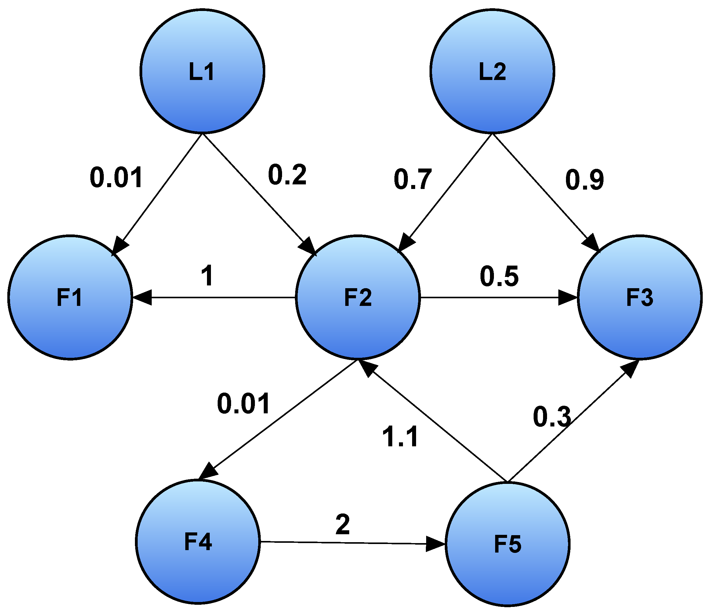
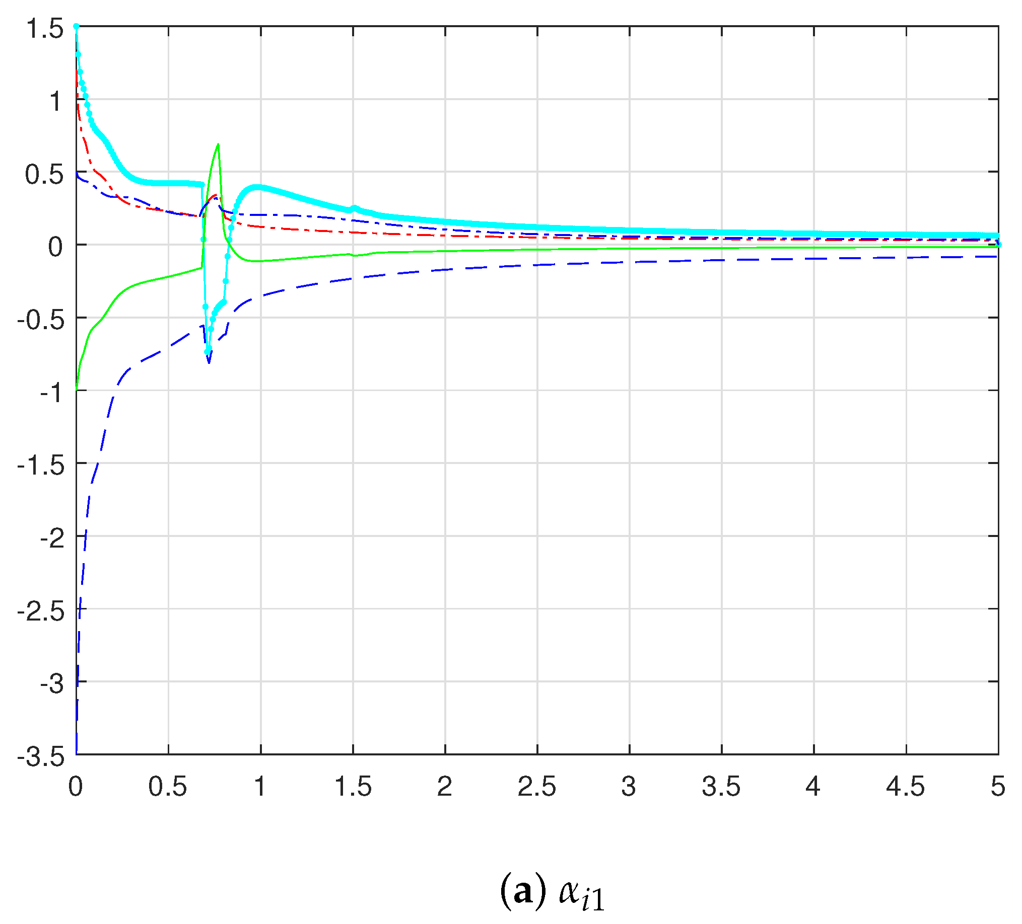
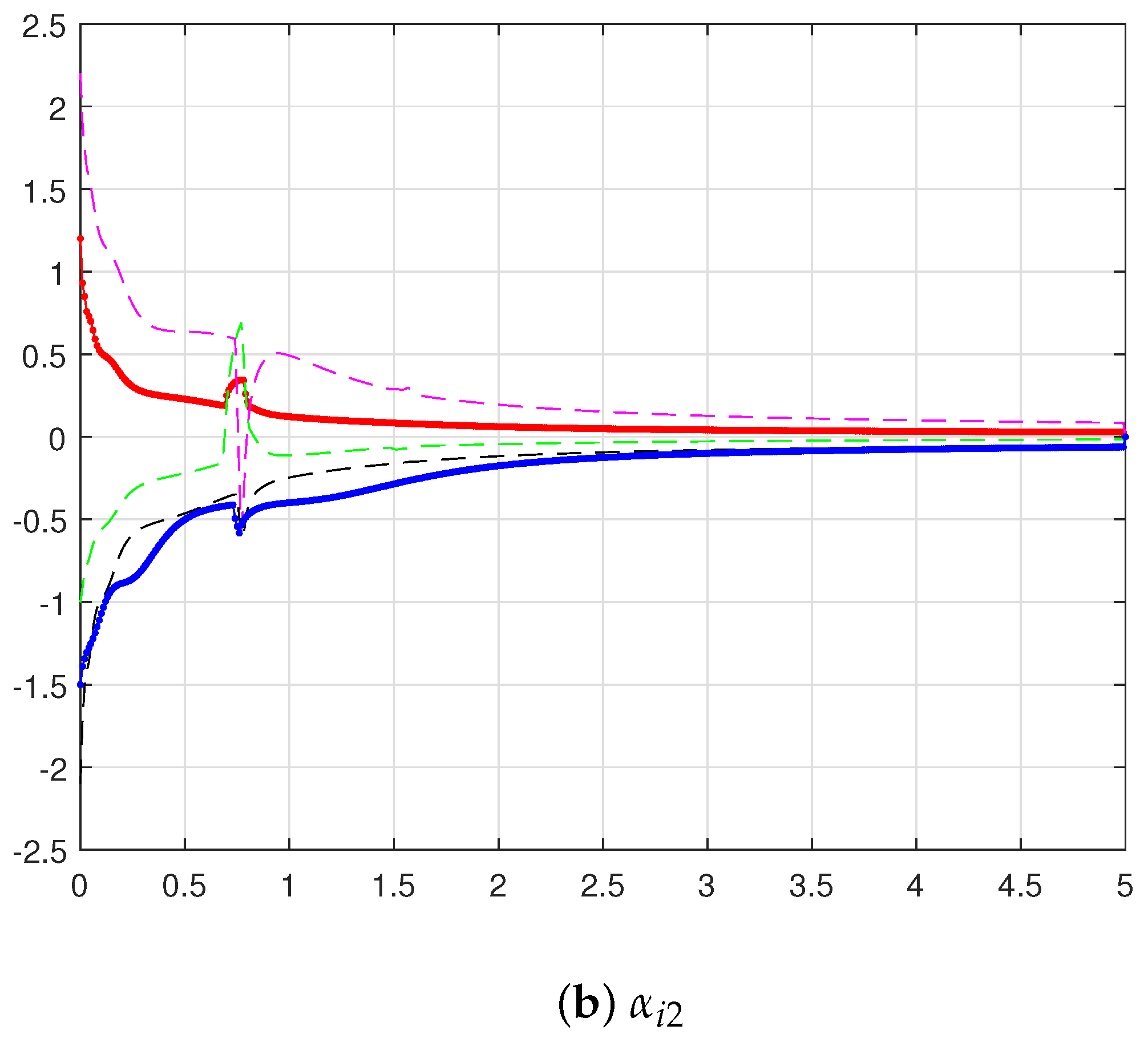
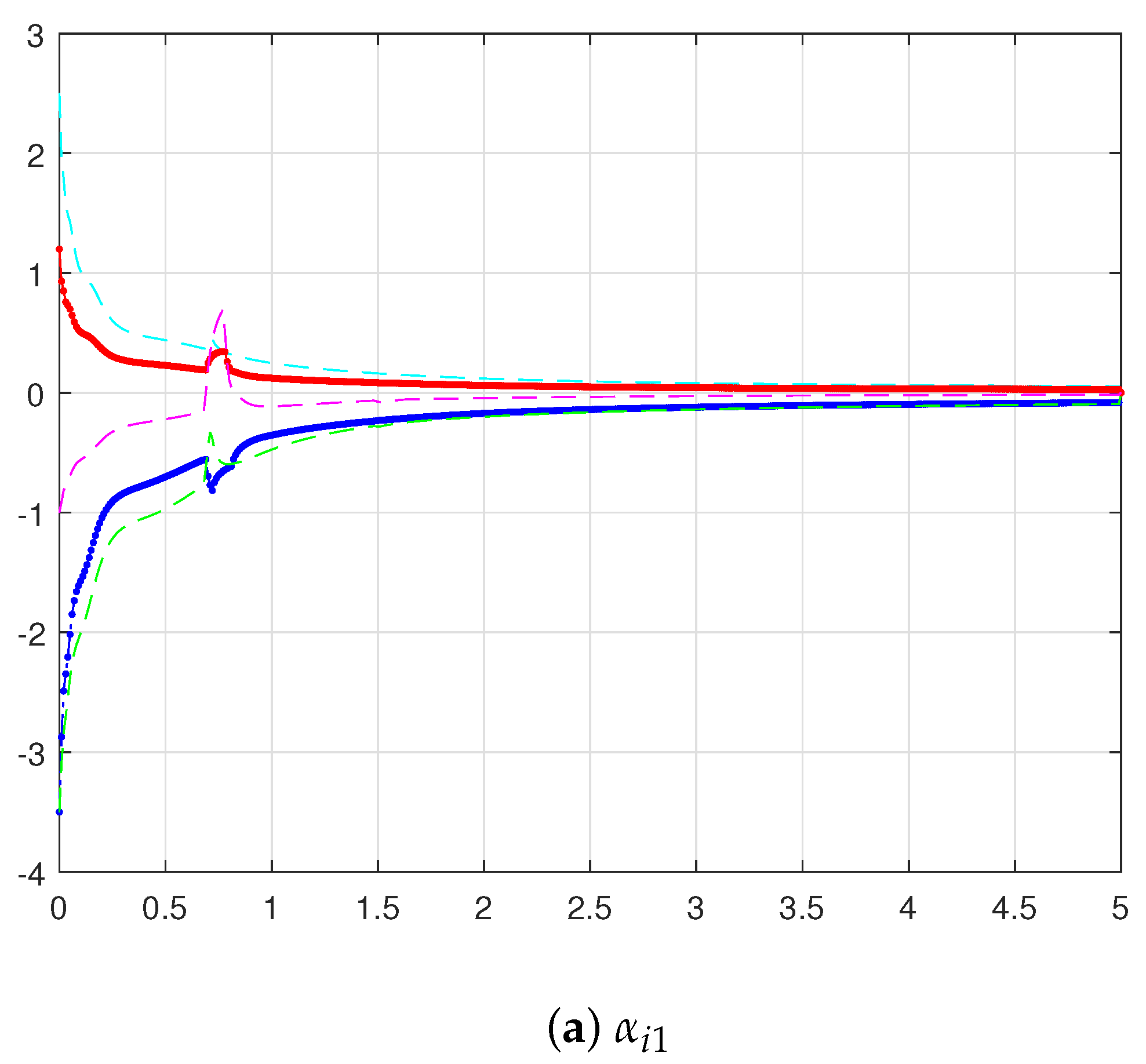
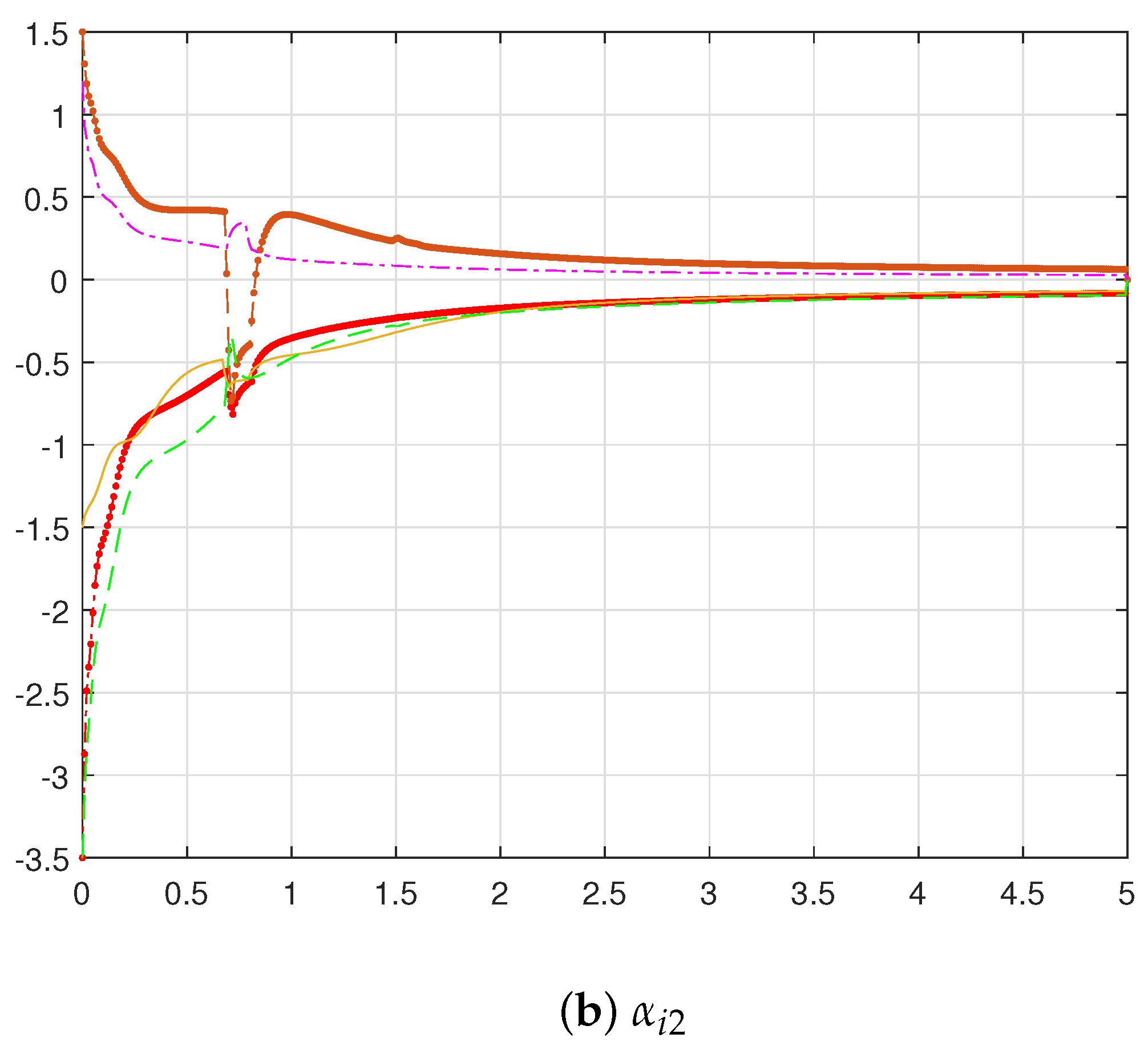
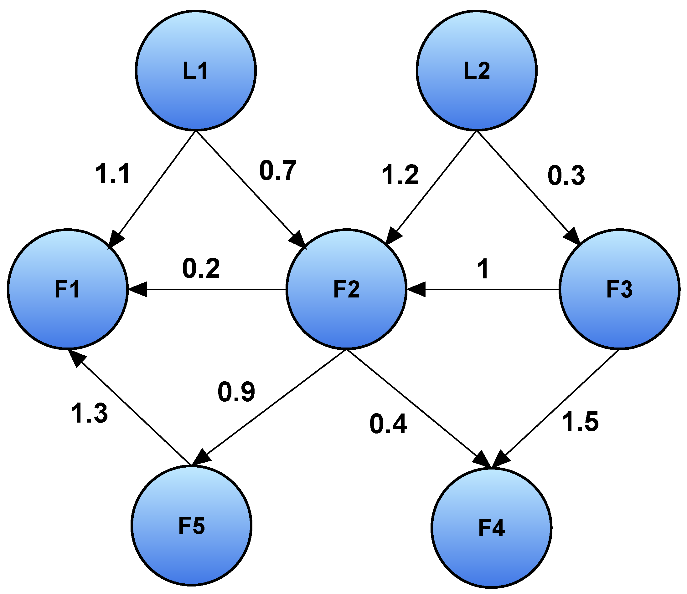
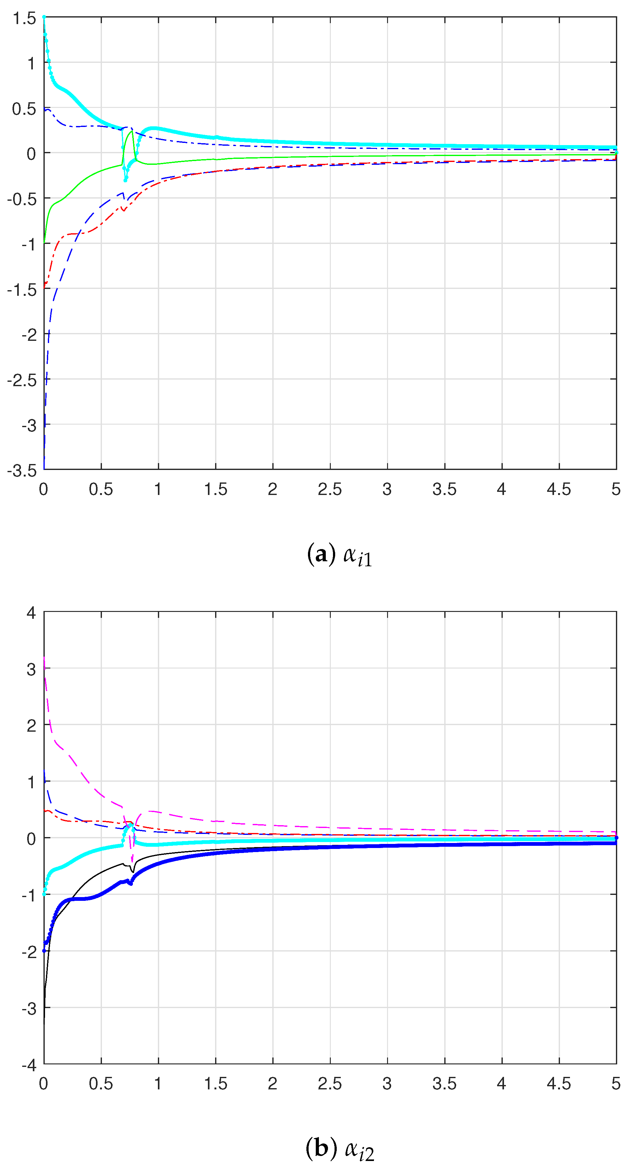
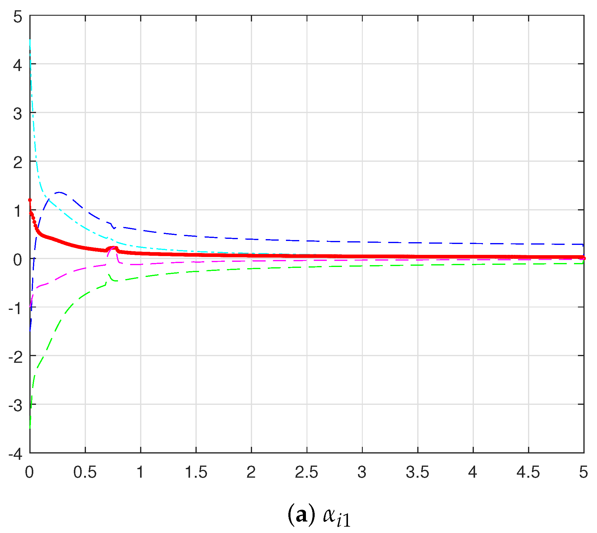
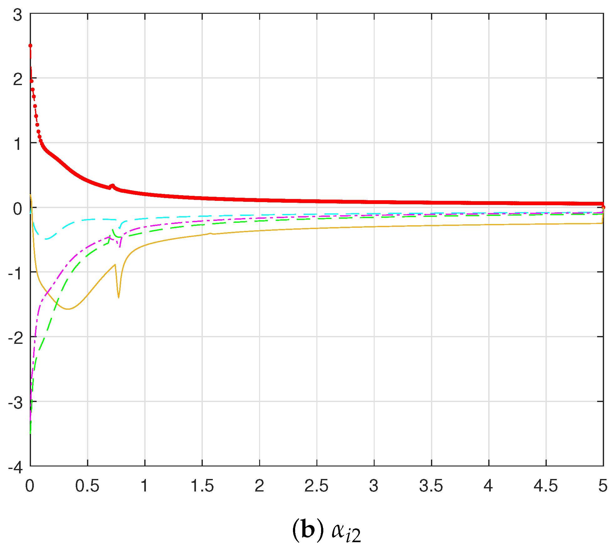
Example 1.
Consider FOMAS (3) with five followers and two leaders describe as Figure 1, where A , B , C R n × n are constant matrices.
A = 1 0 0.1 3
B = 2 0 0.1 1
C = 0.25 0.5 1.3 0
According to Figure 1 one has
L = L F L R 0 0
L = 1.01 1 0 0 0 0.01 0 0 2 0 0 1.1 0.2 0.7 0 0.5 1.7 0 0.3 0 0.9 0 0.03 0 0.03 0 0 0 0 0 0 2 2 0 0 0 0 0 0 0 0 0 0 0 0 0 0 0 0
According to the Schur lemma, association (8) and (9) are equivalent to the inequalities
[ I F [ P A + A T P + ( η 1 + η 2 r 2 ) P + α 1 ( P + P T ) Δ ω ( t ) ] L F ( P K ) L F T ( K T P ) ] ( η 1 ( I F P ) ) ( I F ( P B ) ) ( I F B T P ) < 0 I F [ P A + A T P + ( η 1 + η 2 r 2 ) P + α 1 ( P + P T ) Δ ω ( t ) ] L F ( P K ) L F T ( K T P ) ] ( η 1 ( I F P ) ) < [ I F ( P B B T P ) ] I F [ P A + A T P + ( η 1 + η 2 r 2 ) P + α 1 ( P + P T ) Δ ω ( t ) ] L F ( P K ) L F T ( K T P ) < 1 η 1 [ I F ( P B P 1 B T P ) ] I N [ P A + A T P + ( η 1 + η 2 r 2 ) P + α 1 ( P + P T ) Δ ω ( t ) ] L F ( P K ) L F T ( K T P ) + 1 η 1 [ I F ( P B P 1 B T P ) ] < 0
[ ( η 3 η 2 ) ( I F P ) ( η 3 ( I F P ) ) ] ( I F ( P C ) ) ( I F ( C T P ) ) < 0 ( η 3 η 2 ) ( I F P ) ( η 3 ( I F P ) ) < [ I F ( P C C T P ) ] ( η 3 η 2 ) ( I F P ) < 1 η 3 [ I F ( P C P 1 C T P ) ] ( η 3 η 2 ) ( I F P ) + 1 η 3 [ I F ( P C P 1 C T P ) ] < 0
Choose P = 0.1 1 1 0.1 , η 1 = 2 , η 2 = 3 , η 3 = 2 a n d r 2 = 0.3 . T h e n , K = 0.01 1 0.5 0.01 can be chosen to satisfy (31) and (32), where K R n × n i s t h e g a i n m a t r i x and P is the n × n matrix.
From Equation (32) we have
0.1118897306 0.7830639731 0.7830639731 0.1493063973 < 0
Thus, Theorem (1) is used to achieve CC of FOMAS (3). If we assume that β = 0.6 and r 1 = 0.4 , Figure 2 displays the error α i ( t ) .
On contrary, the Schur lemma demonstrates that mutual relations between (20) and (21) are equivalent to the inequalities
I F [ P A + A T P + ( η 1 + η 2 r ) P + α 1 ( t ) ( P + P T ) Δ ω ( t ) ] ( η 1 ( I F P ) ) ( I F ( P B ) L F ( P K 1 ) ) ( I F ( B T P ) L F T ( K 1 T P ) ) < 0
I F [ P A + A T P + ( η 1 + η 2 r ) P + α 1 ( t ) ( P + P T ) Δ ω ( t ) ] ( η 1 ( I F P ) ) < ( I F ( P B ) L F ( P K 1 ) ) ( I F ( B T P ) L F T ( K 1 T P ) ) I F [ P A + A T P + ( η 1 + η 2 r ) P + α 1 ( t ) ( P + P T ) Δ ω ( t ) ] ( η 1 ( I F P ) ) < [ I F ( P B B T P ) L F T ( P B K 1 T P ) L F ( P K 1 B T P ) + L F L F T ( P K 1 K 1 T P ) ]
I F [ P A + A T P + ( η 1 + η 2 r ) P + α 1 ( t ) ( P + P T ) Δ ω ( t ) ] < 1 η 1 [ I F ( P B P 1 B T P ) L F T ( P B P 1 K 1 T P ) L F ( P K 1 P 1 B T P ) + L F L F T ( P K 1 P 1 K 1 T P ) ]
I F [ P A + A T P + ( η 1 + η 2 r ) P + α 1 ( t ) ( P + P T ) Δ ω ( t ) ] + 1 η 1 [ I F ( P B P 1 B T P ) L F T ( P B P 1 K 1 T P ) L F ( P K 1 P 1 B T P ) + L F L F T ( P K 1 P 1 K 1 T P ) ] < 0
I F [ P A + A T P + ( η 1 + η 2 r ) P + α 1 ( t ) ( P + P T ) Δ ω ( t ) + 1 η 1 ( P B P 1 B T P ) ] + 1 η 1 [ ( L F L F T ) ( P K 1 P 1 K 1 T P ) L F ( P K 1 P 1 B T P ) L F T ( P B P 1 K 1 T P ) ] < 0
( η 3 η 2 ) ( I F P ) ( η 3 ( I F P ) ) ( I F ( P C ) ) ( I F ( C T P ) ) < 0 ( η 3 η 2 ) ( I F P ) ( η 3 ( I F P ) ) ( I F ( P C C T P ) ) < 0 ( η 3 η 2 ) ( I F P ) ( η 3 ( I F P ) ) < ( I F ( P C C T P ) ) ( η 3 η 2 ) ( I F P ) < 1 η 3 ( I F ( P C P 1 C T P ) ) ( η 3 η 2 ) ( I F P ) + 1 η 3 ( I F ( P C P 1 C T P ) ) < 0 I F [ ( η 3 η 2 ) P + 1 η 3 ( P C P 1 C T P ) ] < 0 .
Choose P = 1 0.1 0.1 1 , η 1 = 2 , η 2 = 3 , η 3 = 2 a n d r = 0.3 . T h e n , K 1 = 0.3 0.3 0 0.3 can be chosen to satisfy (33) and (34), where K 1 R n × n and P is an n × n matrix.
From Equation (34) we have
0.5976190476 0.8445238095 0.8445238095 0.2754047619 < 0
Thus, Corollary (1) is used to achieve resilient base CC of FOMAS (3). Taking β = 0.6 , Figure 3 shows the error α i ( t ) .
Example 2.
We examine FOMAS (3) with five followers and two leaders, as shown in Figure 1, where A , B , C R n × n are constant matrices.
A = 6 0 4 7
B = 2 0.3 2 0.2
C = 0.26 0.16 0.6 0.6
According to Figure 4, one has
L = L F L R 0 0
L = 2.6 0.2 0 0 1.3 1.1 0 0 2.9 1 0 0 0.7 1.2 0 0 0.3 0 0 0 0.3 0 0.4 1.5 1.9 0 0 0 0 0.9 0 0 0.9 0 0 0 0 0 0 0 0 0 0 0 0 0 0 0 0
The Schur lemma implies that relationship (8) and (9) are equivalent to the inequalities
[ I F [ P A + A T P + ( η 1 + η 2 r 2 ) P + α 1 ( P + P T ) Δ ω ( t ) ] L F ( P K ) L F T ( K T P ) ] ( η 1 ( I F P ) ) ( I F ( P B ) ) ( I F B T P ) < 0 [ I F [ P A + A T P + ( η 1 + η 2 r 2 ) P + α 1 ( P + P T ) Δ ω ( t ) ] L F ( P K ) L F T ( K T P ) ] ( η 1 ( I F P ) ) < [ I F ( P B B T P ) ] I F [ P A + A T P + ( η 1 + η 2 r 2 ) P + α 1 ( P + P T ) Δ ω ( t ) ] L F ( P K ) L F T ( K T P ) < 1 η 1 [ I F ( P B P 1 B T P ) ] I N [ P A + A T P + ( η 1 + η 2 r 2 ) P + α 1 ( P + P T ) Δ ω ( t ) ] L F ( P K ) L F T ( K T P ) + 1 η 1 [ I F ( P B P 1 B T P ) ] < 0
[ ( η 3 η 2 ) ( I F P ) ( η 3 ( I F P ) ] ( I F ( P C ) ) ( I F ( C T P ) ) < 0 ( η 3 η 2 ) ( I F P ) ( η 3 ( I F P ) ) < [ I F ( P C C T P ) ] ( η 3 η 2 ) ( I F P ) < 1 η 3 [ I F ( P C P 1 C T P ) ] ( η 3 η 2 ) ( I F P ) + 1 η 3 [ I F ( P C P 1 C T P ) ] < 0
Choose P = 2 0.2 0.2 2 , η 1 = 1.6 , η 2 = 2.1 , η 3 = 1.1 a n d r 2 = 0.5 . T h e n , K = 0.2 0.2 0.4 0.2 can be chosen to satisfy (31) and (32), where K R n × n is the gain matrix and P is n × n matrix. From Equation (32) we have
1.8391919192 0.157519192 0.157519194 0.4249519198 < 0
Thus, Theorem (1) is used to achieve CC of FOMAS (3). If we assume that β = 0.6 and r 1 = 0.4 , Figure 5 displays the error α i ( t ) .
Conversely, the Schur lemma shows that relations (20) and (21) are equivalent to the inequalities
I F [ P A + A T P + ( η 1 + η 2 r ) P + α 1 ( t ) ( P + P T ) Δ ω ( t ) ] ( η 1 ( I F P ) ) ( I F ( P B ) L F ( P K 1 ) ) ( I F ( B T P ) L F T ( K 1 T P ) ) < 0
I F [ P A + A T P + ( η 1 + η 2 r ) P + α 1 ( t ) ( P + P T ) Δ ω ( t ) ] ( η 1 ( I F P ) ) < ( I F ( P B ) L F ( P K 1 ) ) ( I F ( B T P ) L F T ( K 1 T P ) ) I F [ P A + A T P + ( η 1 + η 2 r ) P + α 1 ( t ) ( P + P T ) Δ ω ( t ) ] ( η 1 ( I F P ) ) < [ I F ( P B B T P ) L F T ( P B K 1 T P ) L F ( P K 1 B T P ) + L F L F T ( P K 1 K 1 T P ) ]
I F [ P A + A T P + ( η 1 + η 2 r ) P + α 1 ( t ) ( P + P T ) Δ ω ( t ) ] < 1 η 1 [ I F ( P B P 1 B T P ) L F T ( P B P 1 K 1 T P ) L F ( P K 1 P 1 B T P ) + L F L F T ( P K 1 P 1 K 1 T P ) ]
I F [ P A + A T P + ( η 1 + η 2 r ) P + α 1 ( t ) ( P + P T ) Δ ω ( t ) ] + 1 η 1 [ I F ( P B P 1 B T P ) L F T ( P B P 1 K 1 T P ) L F ( P K 1 P 1 B T P ) + L F L F T ( P K 1 P 1 K 1 T P ) ] < 0
I F [ P A + A T P + ( η 1 + η 2 r ) P + α 1 ( t ) ( P + P T ) Δ ω ( t ) + 1 η 1 ( P B P 1 B T P ) ] + 1 η 1 [ ( L F L F T ) ( P K 1 P 1 K 1 T P ) L F ( P K 1 P 1 B T P ) L F T ( P B P 1 K 1 T P ) ] < 0
( η 3 η 2 ) ( I F P ) ( η 3 ( I F P ) ) ( I F ( P C ) ) ( I F ( C T P ) ) < 0 ( η 3 η 2 ) ( I F P ) ( η 3 ( I F P ) ) ( I F ( P C C T P ) ) < 0 ( η 3 η 2 ) ( I F P ) ( η 3 ( I F P ) ) < ( I F ( P C C T P ) ) ( η 3 η 2 ) ( I F P ) < 1 η 3 ( I F ( P C P 1 C T P ) ) ( η 3 η 2 ) ( I F P ) + 1 η 3 ( I F ( P C P 1 C T P ) ) < 0 I F [ ( η 3 η 2 ) P + 1 η 3 ( P C P 1 C T P ) ] < 0 .
Choose P = 3 0.2 0.2 0.9 , η 1 = 3 , η 2 = 4 , η 3 = 3 a n d r = 0.5 . T h e n , K 1 = 0.4 0.4 0 0.4 can be chosen to satisfy (33) and (34), where K 1 R n × n is the gain matrix and P is the n × n matrix. From Equation (34) we have
2.8353834587 0.1094255639 0.1094255639 0.7361483703 < 0
Thus, Corollary (1) is used to achieve resilient base CC of FOMAS (3). Taking β = 0.8 , Figure 6 shows the errors α i ( t ) .

5. Conclusions

We have provided an easy and effective way to look into the resilient base CC of fractional order multi-agent system with mixed time delays. In order to achieve resilient base CC, both delayed and non-delayed control protocols are used. By applying graph theory, the fractional Razumikhin technique and the Lyapunov function technique, certain useful algebraic criteria have been proposed to ensure resilient base CC. Delayed and non delayed control protocol with disturbance term have been designed to solve resilient base containment control. An additional numerical example demonstrates the reliability of the results presented and it is easy to verify the criteria using matrix inequalities. Our approach offers a reliable and easy method to overcome the problems resulting from fractional derivatives and time delays. Our upcoming research will concentrate on CC of single delayed fractional order multi-agent systems that are nonlinear.

Author Contributions

Conceptualization, W.A.; Software, W.A.; Validation, A.K.; Formal analysis, J.A.M.; Resources, A.K.; Data curation, J.A.M.; Writing—original draft, A.J.; Writing-review & editing, A.U.K.N.; Supervision, A.U.K.N.; Project administration, A.K. All authors have read and agreed to the published version of the manuscript.

Funding

This research was sponsored by the Guangzhou Government Project under Grant No. 62216235, and the National Natural Science Foundation of China (Grant No. 622260-1).

Conflicts of Interest

The authors declare that they have no known competing financial interests or personal relationships that could have appeared to influence the work reported in this paper.

References

  1. Pakdeetrakulwong, U.; Wongthongtham, P.; Siricharoen, W.; Khan, N. An ontology-based multi-agent system for active software engineering ontology. Mob. Netw. Appl. 2016, 21, 65–88. [Google Scholar] [CrossRef]
  2. Jia, J.; Huang, X.; Li, Y.; Cao, J.; Ahmed, A. Global stabilization of fractional-order memristor-based neural networks with time delay. IEEE Trans. Neural Netw. Learn. Syst. 2020, 31, 997–1009. [Google Scholar] [CrossRef] [PubMed]
  3. Han, S.K. Prescribed consensus and formation error constrained finite-time sliding mode control for multi-agent mobile robot systems. IET Control Theory Appl. 2018, 12, 282–290. [Google Scholar] [CrossRef]
  4. Krzysztof, M. A computer simulation of traffic flow with on-street parking and drivers’ behaviour based on cellular automata and a multi-agent system. J. Comput. Sci. 2018, 28, 32–42. [Google Scholar]
  5. Yang, R.; Liu, S.; Tan, Y.Y.; Zhan, Y.J.; Jiang, W. Consensus analysis of fractional-order nonlinear multi-agent systems with distributed and input delays. Neurocomputing 2019, 329, 46–52. [Google Scholar] [CrossRef]
  6. Xie, X.; Mu, X. Leader-following consensus of nonlinear singular multiagent systems with intermittent communication. Math. Methods Appl. Sci. 2019, 42, 2877–2891. [Google Scholar] [CrossRef]
  7. Tan, X.; Cao, J.; Li, X.; Alsaedi, A. Leader-following mean square consensus of stochastic multi-agent systems with input delay via event-triggered control. IET Control Theory Appl. 2018, 12, 299–309. [Google Scholar] [CrossRef]
  8. Sakthivel, R.; Kaviarasan, B.; Lee, H.; Lim, Y. Finite-time leaderless consensus of uncertain multi-agent systems against time-varying actuator faults. Neurocomputing 2019, 325, 159–171. [Google Scholar] [CrossRef]
  9. Qin, J.; Yu, C.; Anderson, B. On leaderless and leader-following consensus for interacting clusters of second-order multi-agent systems. Automatica 2016, 74, 214–221. [Google Scholar] [CrossRef]
  10. Shang, Y. Hybrid consensus for averager-copier-voter networks with non-rational agents. Chaos Solitons Fractals 2018, 110, 244–251. [Google Scholar] [CrossRef]
  11. Wang, Y.; Song, Y.; Krstic, M. Collectively rotating formation and containment deployment of multiagent systems: A polar coordinate-based finite time approach. IEEE Trans. Cybern. 2017, 47, 2161–2172. [Google Scholar] [CrossRef]
  12. Duan, Y.; Cui, B.X.; Xu, X.H. A multi-agent reinforcement learning approach to robot soccer. Artif. Intell. Rev. 2012, 38, 193–211. [Google Scholar] [CrossRef]
  13. Ye, D.; Chen, M.; Li, K. Observer-based distributed adaptive fault-tolerant containment control of multiagent systems with general linear dynamics. ISA Trans. 2017, 71, 32–39. [Google Scholar] [CrossRef]
  14. Zuo, S.; Song, Y.; Lewis, F.; Davoudi, A. Adaptive output containment control of heterogeneous multiagent systems with unknown leaders. Automatica 2018, 92, 235–239. [Google Scholar] [CrossRef]
  15. Liu, H.; Cheng, L.; Tan, M.; Hou, Z.G. Containment control of continuous-time linear multi-agent systems with aperiodic sampling. Automatica 2015, 57, 78–84. [Google Scholar] [CrossRef]
  16. Xia, H.; Zheng, W.X.; Shao, J. Event-triggered containment control for second-order multi-agent systems with sampled position data. ISA Trans. 2017, 73, 91–99. [Google Scholar] [CrossRef]
  17. Liu, Y.; Su, H. Containment control of second-order multi-agent systems via intermittent sampled position data communication. Appl. Math. Comput. 2019, 362, 124522. [Google Scholar] [CrossRef]
  18. Wang, D.; Huang, Y.; Guo, S.; Wang, W. Distributed H(infinity) containment control of multi-agent systems over switching topologies with communication time delay. Int. J. Robust Nonlinear Control 2020, 30, 5221–5232. [Google Scholar] [CrossRef]
  19. Han, T.; Li, J.; Guan, Z.H.; Cai, Z.X.; Zhang, D.X.; He, D.X. Containment control of multi-agent systems via a disturbance observer-based approach. J. Frankl. Inst. 2019, 356, 2919–2933. [Google Scholar] [CrossRef]
  20. He, X.; Wang, Q.; Yu, W. Distributed finite-time containment control for second-order nonlinear multiagent systems. Appl. Math. Comput. 2015, 268, 509–521. [Google Scholar]
  21. Huang, C.; Li, H.; Li, T.; Chen, S. Stability and bifurcation control in a fractional predator-prey model via extended delay feedback. Int. J. Bifurc. Chaos 2019, 29, 1950150. [Google Scholar] [CrossRef]
  22. Luo, D.; Wang, J.R.; Shen, D. Learning formation control for fractional-order multiagent systems. Math. Methods Appl. Sci. 2018, 41, 5003–5014. [Google Scholar] [CrossRef]
  23. Zhang, H.; Ye, R.; Cao, J.; Ahmed, A.; Li, X.; Wan, Y. Lyapunov functional approach to stability analysis of Riemann-Liouville fractional neural networks with time-varying delays. Asian J. Control 2017, 20, 1938–1951. [Google Scholar] [CrossRef]
  24. Caputo, M.; Fabrizio, M. On the notion of fractional derivative and applications to the hysteresis phenomena. Meccanica 2017, 52, 3043–3052. [Google Scholar] [CrossRef]
  25. Yang, H.; Yang, Y.; Han, F.; Zhao, M.; Guo, L. Containment control of heterogeneous fractional-order multi-agent systems. J. Frankl. Inst. 2019, 356, 752–765. [Google Scholar] [CrossRef]
  26. Zou, W.; Xiang, Z. Containment control of fractional-order nonlinear multi-agent systems under fixed topologies. IMA J. Math. Control Inf. 2018, 35, 1027–1041. [Google Scholar] [CrossRef]
  27. Yuan, X.L.; Mo, L.P.; Yu, Y.G.; Ren, G.J. Distributed containment control of fractional-order multiagent systems with double-integrator and nonconvex control input constraints. Int. J. Control Autom. Syst. 2020, 18, 1728–1742. [Google Scholar] [CrossRef]
  28. Liu, F.; Dong, T.; Guan, Z.H.; Wang, H.O. Stability analysis and bifurcation control of a delayed incommensurate fractional-order gene regulatory network. Int. J. Bifurc. Chaos 2020, 30, 2050089. [Google Scholar] [CrossRef]
  29. Liu, S.; Yang, R.; Zhou, X.F.; Jiang, W.; Li, X.; Zhao, X.W. Stability analysis of fractional delayed equations and its applications on consensus of multi-agent systems. Commun. Nonlinear Sci. Numer. Simul. 2019, 73, 351–362. [Google Scholar] [CrossRef]
  30. Liu, H.; Xie, G.; Yu, M. Necessary and sufficient conditions for containment control of fractional-order multi-agent systems. Neurocomputing 2018, 323, 86–95. [Google Scholar] [CrossRef]
  31. Liu, H.; Xie, G.; Gao, Y. Containment control of fractional-order multi-agent systems with time-varying delays. J. Frankl. Inst. 2019, 356, 9992–10014. [Google Scholar] [CrossRef]
  32. Chen, J.; Guan, Z.H.; Yang, C.; Li, T. Distributed containment control of fractional-order uncertain multi-agent systems. J. Frankl. Inst. 2016, 353, 1672–1688. [Google Scholar] [CrossRef]
  33. Yang, H.; Wang, F.; Han, F. Containment Control of fractional order multi-agent systems with time delays. IEEE J. Autom. Sin. 2018, 5, 727–732. [Google Scholar] [CrossRef]
  34. Podlubny, I. Fractional Differential Equations; Academic Press: New York, NY, USA, 1999. [Google Scholar]
  35. Mei, J.; Ren, W.; Ma, G. Distributed containment control for Lagrangian networks with parametric uncertainties under a directed graph. Automatica 2012, 48, 653–659. [Google Scholar] [CrossRef]
  36. Manuel, A.; Norelys, A.; Javier, A.; Rafael, C. Using general quadratic Lyapunov functions to prove Lyapunov uniform stability for fractional order systems. Commun. Nonlinear Sci. Numer. Simul. 2015, 22, 650–659. [Google Scholar]
  37. Hu, J.; Yu, J.; Cao, J. Distributed containment control for nonlinear multi-agent systems with time-delayed protocol. Asian J. Control 2015, 18, 747–756. [Google Scholar] [CrossRef]
Figure 1. Communication topology of FOMAS (3) consisting of leader and follower is a weighted digraph.
Fractalfract 07 00409 g001
Figure 2. Resilient base CC errors α i ( t ) = ( α i 1 T ( t ) , α i 2 T ( t ) ) T of FOMAS (3) under communication topology with non delayed control protocol (4).
Fractalfract 07 00409 g002aFractalfract 07 00409 g002b
Figure 3. Resilient base CC errors α i ( t ) of FOMAS (3) under communication topology with delayed control protocol (12).
Fractalfract 07 00409 g003aFractalfract 07 00409 g003b
Figure 4. Communication topology of FOMAS (3) shows the arrangement of vertices in the network.
Fractalfract 07 00409 g004
Figure 5. Graph represents resilient base CC errors α i ( t ) = ( α i 1 T ( t ) , α i 2 T ( t ) ) T of FOMAS (3) under communication topology with non delayed control protocol (4).
Fractalfract 07 00409 g005
Figure 6. Graph represents resilient base CC error α i ( t ) of FOMAS (3) under communication topology with delayed control protocol (12).
Fractalfract 07 00409 g006aFractalfract 07 00409 g006b
Disclaimer/Publisher’s Note: The statements, opinions and data contained in all publications are solely those of the individual author(s) and contributor(s) and not of MDPI and/or the editor(s). MDPI and/or the editor(s) disclaim responsibility for any injury to people or property resulting from any ideas, methods, instructions or products referred to in the content.

