Pitch Angle Control of an Airplane Using Fractional Order Direct Model Reference Adaptive Controllers

Abstract

This paper deals with the longitudinal movement control of an airplane (pitch angle) using fractional order adaptive controllers (FOACs). It shows the improvements achieved in the plane’s behavior, in terms of the minimization of a given performance index. At the same time, less control effort is needed to accomplish the control objectives compared with the classic integer order adaptive controllers (IOACs). In this study, fractional order direct model reference adaptive control (FO-DMRAC) is implemented at the simulation level, and exhibits a better performance compared with the classic integer order (IO) version of the DMRAC (IO-DMRAC). It is also shown that the proposed control strategy for FO-DMRAC reduces the resultant system control structure down to a relative degree 2 system, for which the control implementation is simpler and avoids oscillations during the transient period. Moreover, it is interesting to note that this is the first time that an FOAC with fractional adaptive laws is applied to the longitudinal control of an airplane. A suitable model for the longitudinal movement of the airplane related to the pitch angle θ as the output variable with the lifter angle (δe) as the control variable, is first analyzed and discussed to obtain a reliable mathematical model of the plane. All of the other input variables acting on the plane are considered as perturbations. For certain operating conditions defined by the flight conditions, an FO-DMRAC is designed, simulated, and analyzed. Furthermore, a comparison with the implementation of the classical adaptive general direct control (relative degree ≥ 2) is presented. The boundedness and convergence of all of the signals are theoretically proven based on the new Lemma 3, assuring the boundedness of all internal signals ω(t).

1. Introduction

Controlling the pitch angle $\theta \left(t\right)$ (attitude) of an aircraft (see Figure 1) is relevant in the aviation industry, since an important part of the pilots’ tasks is to maintain a specific attitude, that is to say, to achieve a straight and level flight, as well as to ascend or to descend with a certain angle $\theta$ (attitude) with respect to the horizon. Since these tasks require the pilot to be diligent, most sophisticated aircraft have an autopilot attitude to complete the job and achieve the following goals:

-

To relieve the pilot from manipulating the controls, reducing the loads on the plane, and improving navigation accuracy;

-

To fly the airplane without direct control over the longitudinal control surfaces (elevator or tail).

Small planes widely use classical controllers, such as proportional-integral-derivative (PID) controllers because of their simplicity to maintain the airplane under control [1,2,3,4,5]. The main disadvantage is that they do not have adaptation capabilities to face large variations in the operating conditions, external perturbations acting on the plane, or eventual plane parameter variations, since PID parameters are fixed.

In controlling plane trajectories, rather simple controllers, such as the integer order (IO) PID have been reported in the control literature. Only a few attempts have been made to use adaptive or more complex control strategies [6,7,8,9]. Moreover, techniques, such as μ-synthesis [10] and nonlinear control [11] have also been used to control airplanes with good results. In [11], a tracking controller consisting of feedforward and static state feedback was designed to guarantee uniform asymptotic trajectory tracking. The landing control of an F-18 fighter aircraft based on a PID controller with an active disturbance rejection (ADR) system was studied in [12]. In [13], an LQR controller based on genetic algorithms was designed for the longitudinal control of an F-16 fighter aircraft under different flight regimes. The longitudinal control of a B-1 bomber was analyzed in [14] using an optimal multivariable control approach [15,16,17] of the LQG/LTR type based on an adaptive observer [18,19].

Furthermore, in [9,12], the longitudinal control of an F-16 Falcon fighter aircraft was studied by applying advanced control techniques, such as MRAC in its combined version (CMRAC), which could serve as a basis for comparison for an extension of the CMRAC techniques to the fractional order case (FO-CMRAC).

Additionally, in [20], the longitudinal control using backstepping control was applied to a model X-plane similar to the NexStar plane with rectangular wings. In [21], the longitudinal and lateral control of unmanned vehicles, such as helicopters, were studied. The control approach used is of the adaptive type based on a continuous linearization for different operating points to then apply MRAC.

In [22], a typical MRAC approach was used (integer order plant and integer adaptive control laws) for the longitudinal control of an F-15 aircraft and the fractional part of this work was the fractional filter that approximates the plant that is newly approximate to an integer transfer function of the plant. Moreover, in this work, two new blocks were used (dynamic inversion and PI compensator blocks) achieving a more complex implementation.

It is important to mention that no attempt has been reported in the technical literature about the use of FO adaptive controllers for the longitudinal control of an airplane in which fractional adaptive laws are applied to an integer plant (airplane model) with no other additional special blocks.

The paper is organized as follows. In Section 2, the airplane model used in this study is presented for certain flight conditions and controlled by a standard DMRAC. Section 3 is devoted to the description of the DMRAC strategy. Section 4 presents some basic concepts of fractional order calculus that will be used in this study, and a new lemma (Lemma 3) that relaxes the stability condition is proposed. In Section 5, several simulation results are presented with numerical values of the parameters corresponding to the Cessna 182 plane used in this study [2]. Finally, in Section 6, some conclusions are drawn.

2. General Concepts on Plane Dynamics and Flight Control

2.1. Mathematical Model of the Longitudinal Movement of a Plane

In this Section, the basic concepts of a plane’s dynamics and its control are presented. In many cases, plane dynamic motion can be modeled assuming small disturbances concerning the airplane’s static stable path (operating point). The differential equations used in this study represent only the plane’s longitudinal movement, although the complete movement is in three dimensions. These equations are considered linear (or linearized) with constant coefficients corresponding to small deviations in the airplane’s operating point.

We consider the static stable path condition of a straight and level flight. The movement equations must consider the aerodynamic force and moment disturbances. By choosing ${\omega }_1=0$ (angular velocity along the z-axis in rad/s), we obtain the plane small disturbances longitudinal equations separated from the small disturbances directional-lateral equations [2].

Next, for a better understanding of the variables in the equations that follow,

Table 1. Glossary of terms used in the control of the Cessna-182.

Variable	Meaning	Variable	Meaning
${\theta }_1 \left[\mathrm{r}\mathrm{a}\mathrm{d}\right]$	Stationary pitch angle	$Z_{\alpha } [\mathrm{f}\mathrm{t}·\mathrm{r}\mathrm{a}\mathrm{d}/{\mathrm{s}}^2]$	Vertical acceleration per unit angle of attack
$\theta \left[\mathrm{r}\mathrm{a}\mathrm{d}\right]$	Pitch angle or perturbed pitch angle	$Z_{\dot{\alpha }} [\mathrm{f}\mathrm{t}·\mathrm{r}\mathrm{a}\mathrm{d}/\mathrm{s}]$	Vertical acceleration per unit rate change of angle of attack
$U_1 \left[\mathrm{m}\mathrm{p}\mathrm{h}\right]$	Stationary longitudinal velocity	$Z_q [\mathrm{f}\mathrm{t}·\mathrm{r}\mathrm{a}\mathrm{d}/\mathrm{s}]$	Vertical acceleration per unit pitch rate
$u \left[\mathrm{m}\mathrm{p}\mathrm{h}\right]$	Perturbed longitudinal velocity	$Z_{{\delta }_e} [\mathrm{f}\mathrm{t}·\mathrm{r}\mathrm{a}\mathrm{d}/{\mathrm{s}}^2]$	Vertical acceleration per unit elevator angle
$\alpha \left[\mathrm{r}\mathrm{a}\mathrm{d}\right]$	Angle of attack or perturbed angle of attack	$M_u [\mathrm{f}\mathrm{t}·\mathrm{r}\mathrm{a}\mathrm{d}/\mathrm{s}]$	Pitch angular acceleration per speed unit change
$\gamma \left[\mathrm{r}\mathrm{a}\mathrm{d}\right]$	Path flight angle	$M_{T_u} [\mathrm{f}\mathrm{t}·\mathrm{r}\mathrm{a}\mathrm{d}/\mathrm{s}]$	Pitch angular acceleration per unit change in speed (due to thrust)
$g [\mathrm{f}\mathrm{t}/{\mathrm{s}}^2]$	Acceleration of gravity	$M_{\alpha } [1/{\mathrm{s}}^2]$	Pitch angular acceleration per unit angle of attack
$X_u [1/\mathrm{s}]$	Forward acceleration per speed unit change	$M_{T_{\alpha }} [1/{\mathrm{s}}^2]$	Pitch angular acceleration per unit angle of attack (due to thrust)
$X_{T_u} [1/\mathrm{s}]$	Forward acceleration per speed unit change (due to thrust)	$M_{\dot{\alpha }} [1/\mathrm{s}]$	Pitch angular acceleration per unit rate of change of attack angle
$X_{\alpha } [\mathrm{f}\mathrm{t}·\mathrm{r}\mathrm{a}\mathrm{d}/{\mathrm{s}}^2]$	Forward acceleration per unit angle of attack	$M_q [1/\mathrm{s}]$	Pitch angular acceleration per unit pitch rate
$X_{{\delta }_e} [\mathrm{f}\mathrm{t}·\mathrm{r}\mathrm{a}\mathrm{d}/{\mathrm{s}}^2]$	Forward acceleration per unit elevator angle	$M_{{\delta }_e} [1/{\mathrm{s}}^2]$	Pitch angular acceleration per unit elevator angle
$Z_u [1/\mathrm{s}]$	Vertical acceleration per speed unit change

shows the glossary of terms with their respective units used in this paper.

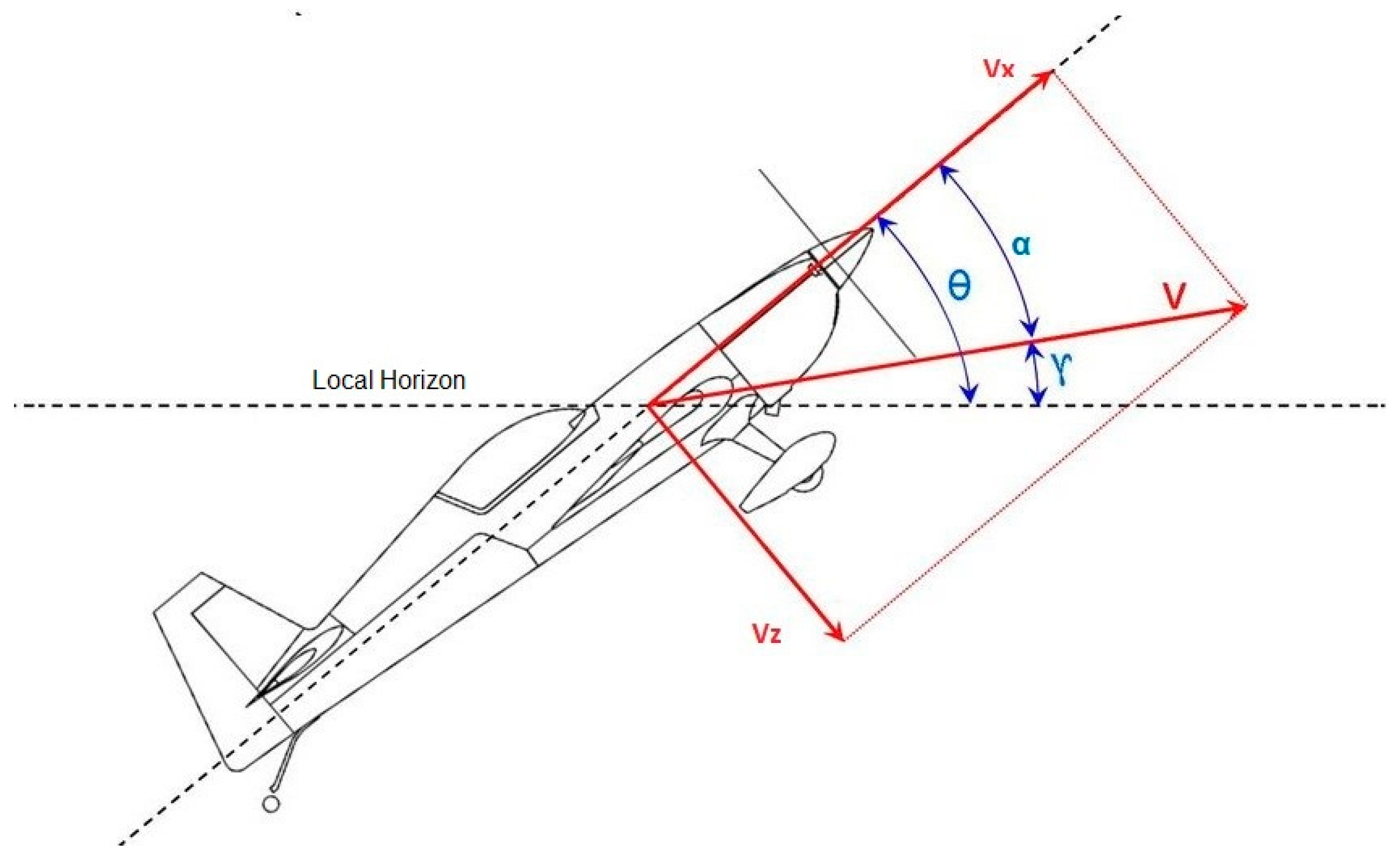
To simplify the analysis, Figure 1 shows the geometry and the longitudinal angles of interest for the aircraft used in this study.

Figure 1. Fundamental angles of the longitudinal movement of an aircraft (figure uploaded by Baron Johnson [23]).

Figure 1. Fundamental angles of the longitudinal movement of an aircraft (figure uploaded by Baron Johnson [23]).

V is the wind speed relative to the aircraft, θ is the pitch angle, α is the angle of attack, and (it is important to note that this symbol is the same as the order of fractional derivatives, nevertheless this should not be confusing because of the context) γ is the flight path angle. Note that $\gamma =\theta -\alpha$.

The airplane used in this study for the simulations of different adaptive control strategies, in its integer and fractional order versions, is the Cessna-182 utility aircraft, which is very popular due to its low cost and high performance. In addition, this aircraft is widely used in the training process for civil pilots.

Using the plane general dynamic equations and the aerodynamic and trust force disturbances, we obtain the following equations describing the plane’s disturbed longitudinal movement [2,8].

$$\begin{array}{l}\dot{u}\left(t\right)=-g\theta \left(t\right)\mathit{cos}{\theta }_1+X_u\cdot u\left(t\right)+X_{T_u}\cdot u\left(t\right)+X_{\alpha }\cdot \alpha \left(t\right)+X_{{\delta }_e}\cdot {\delta }_e\left(t\right),\\ U_1\cdot \dot{\alpha }\left(t\right)-U_1\cdot \dot{\theta }\left(t\right)=-g\cdot \theta \left(t\right)sin{\theta }_1+Z_u\cdot u\left(t\right)+Z_{\alpha }\cdot \alpha \left(t\right)+Z_{\dot{\alpha }}\cdot \dot{\alpha }\left(t\right)+Z_q\cdot \dot{\theta }\left(t\right)+Z_{{\delta }_e}\cdot {\delta }_e\left(t\right),\\ \ddot{\theta }\left(t\right)=M_u\cdot u\left(t\right)+M_{T_u}\cdot u\left(t\right)+M_{\alpha }\cdot \alpha \left(t\right)+M_{T_{\alpha }}\cdot \alpha \left(t\right)+M_{\dot{\alpha }}\cdot \dot{\alpha }\left(t\right)+M_q\cdot \dot{\theta }\left(t\right)+M_{{\delta }_e}\cdot {\delta }_e\left(t\right),\end{array}$$

(1)

where $u\left(t\right)$ is the perturbed linear velocity along the longitudinal axis of the aircraft, $\alpha \left(t\right)$ is the angle of attack, $\theta \left(t\right)$ is the perturbed pitch angle, ${\delta }_e\left(t\right)$ is the tail elevator angle and $X_i\left(t\right)$, $Z_i\left(t\right),$ and $M_i\left(t\right)$ are, respectively, the derivatives of cinematics forward, vertical, and moments variables concerning the variable of interest i.

Then, a linearized model around a specified operating point is defined allowing for the introduction of basic and advanced control concepts for the resulting dynamical system. First, it is convenient to perform the following change of notation:

$$\begin{array}{l}{x}_1\left(t\right)=\theta \left(t\right),\\ x_2(t)=\dot{\theta }\left(t\right),\hspace{0.33em}\\ x_3\left(t\right)=u\left(t\right),\hspace{0.33em}\\ x_4\left(t\right)=\alpha \left(t\right),\end{array}$$

to express the set of Equation (1) in the state space matrix form, represented as:

$$\begin{array}{l}\dot{x}\left(t\right)=A\cdot x\left(t\right)+B\cdot u\left(t\right),\\ y\left(t\right)=C\cdot x\left(t\right),\end{array}$$

where $A,B,\mathrm{and}C$ are the constant matrices of proper dimensions. Following some algebraic manipulation, we arrive at the following system of equations expressed in state variables:

$$\begin{array}{l}{\dot{x}}_1\left(t\right)=x_2\left(t\right),\\ {\dot{x}}_2\left(t\right)=-\frac{gsin{\theta }_1{M}_{\dot{\alpha }}}{Z_{\dot{\alpha }}+U_1}{x}_1\left(t\right)+\left(M_q+M_{\dot{\alpha }}\frac{Z_q+U_1}{Z_{\dot{\alpha }}+U_1}\right)x_2\left(t\right)+\left(M_u+M_{T_u}\frac{M_{\dot{\alpha }}\cdot Z_u}{Z_{\dot{\alpha }}+U_1}\right)x_3\left(t\right),\\ {\dot{x}}_3\left(t\right)=-g\mathit{cos}{\theta }_1{x}_1\left(t\right)+\left(X_u+X_{T_u}\right)x_3\left(t\right)+X_{\alpha }{x}_4\left(t\right)+X_{{\delta }_e}{\delta }_e\left(t\right),\\ {\dot{x}}_4\left(t\right)=-\frac{gsin{\theta }_1}{Z_{\dot{\alpha }}+U_1}{x}_1\left(t\right)+\left(\frac{Z_q+U_1}{Z_{\dot{\alpha }}+U_1}\right)x_2\left(t\right)+\left(\frac{Z_u}{Z_{\dot{\alpha }}+U_1}\right)x_3\left(t\right)+\left(\frac{Z_{\alpha }}{Z_{\dot{\alpha }}+U_1}\right)x_4\left(t\right)+\left(\frac{Z_{{\delta }_e}}{Z_{\dot{\alpha }}+U_1}\right){\delta }_e\left(t\right).\end{array}$$

(2)

The matrix representation of System (2) becomes

$$\begin{gathered} \left[\begin{array}{c}{\dot{x}}_1\\ {\dot{x}}_2\\ {\dot{x}}_3\\ {\dot{x}}_4\end{array}\right]=\left[\begin{array}{cccc}0& 1& 0& 0\\ -\frac{gsin{\theta }_1{M}_{\dot{\alpha }}}{Z_{\dot{\alpha }}+U_1}& M_q+M_{\dot{\alpha }}\frac{Z_q+U_1}{Z_{\dot{\alpha }}+U_1}& M_u+M_{T_u}\frac{M_{\dot{\alpha }}\cdot Z_u}{Z_{\dot{\alpha }}+U_1}& M_{\alpha }+M_{T_{\alpha }}\frac{M_{\dot{\alpha }}\cdot Z_{\alpha }}{Z_{\dot{\alpha }}+U_1}\\ -g\mathit{cos}{\theta }_1& 0& X_u+X_{T_u}& X_{\alpha }\\ -\frac{gsin{\theta }_1}{Z_{\dot{\alpha }}+U_1}& \frac{Z_q+U_1}{Z_{\dot{\alpha }}+U_1}& \frac{Z_u}{Z_{\dot{\alpha }}+U_1}& \frac{Z_{\alpha }}{Z_{\dot{\alpha }}+U_1}\end{array}\right]\left[\begin{array}{c}{x}_1\\ x_2\\ x_3\\ x_4\end{array}\right]+\left[\begin{array}{c}0\\ M_{{\delta }_e}+\frac{M_{\dot{\alpha }}\cdot Z_{{\delta }_e}}{Z_{\dot{\alpha }}+U_1}0\\ X_{{\delta }_e}\\ \frac{Z_{{\delta }_e}}{Z_{\dot{\alpha }}+U_1}\end{array}\right]{\delta }_e\left(t\right), \\ y\left(t\right)=\left[\begin{array}{cccc}1& 0& 0& 0\end{array}\right]\left[\begin{array}{c}{x}_1\\ x_2\\ x_3\\ x_4\end{array}\right], \end{gathered}$$

(3)

where ${\delta }_e\left(t\right)$ is the system input and $y\left(t\right)=\theta \left(t\right)$ is the system output.

The fractional order direct model reference adaptive control (FO-DMRAC) designed for this application will be later compared with its integer order counterpart (IO-DMRAC). The flight conditions will be those corresponding to a straight and level flight, considering the operating conditions shown in

Table 2. Cessna-182 operating conditions in straight and level flight.

Operating Conditions
Altitude [feet]	5.000
Velocity [m.p.h.]	130
Weight [pounds]	2.650
Dynamic Pressure [p.s.i]	49.6
Center of gravity in percent [%]	26.4

.

For more information on the operational and technical characteristics of this aircraft, the reader is referred to [24].

Additionally,

Table 3. Derivative coefficients of the Cessna-182 airplane.

Derivative Coefficients and Values
Derivative Coefficient	Units	Derivative Coefficient	Units
$X_u=-0.95$	$\frac{\mathrm{f}\mathrm{t}/{\mathrm{s}}^2}{\mathrm{f}\mathrm{t}/\mathrm{s}}$	$Z_{\delta e}=0$	$\frac{\mathrm{f}\mathrm{t}/{\mathrm{s}}^2}{\mathrm{r}\mathrm{a}\mathrm{d}}$
$X_{T_u}=0.47$	$\frac{\mathrm{f}\mathrm{t}/{\mathrm{s}}^2}{\mathrm{f}\mathrm{t}/\mathrm{s}}$	$M_u=0$	$\frac{\mathrm{r}\mathrm{a}\mathrm{d}/{\mathrm{s}}^2}{\mathrm{f}\mathrm{t}/\mathrm{s}}$
$X_{\alpha }=605.76$	$\frac{\mathrm{f}\mathrm{t}/{\mathrm{s}}^2}{\mathrm{r}\mathrm{a}\mathrm{d}}$	$M_{T_u}=0$	$\frac{\mathrm{r}\mathrm{a}\mathrm{d}/{\mathrm{s}}^2}{\mathrm{f}\mathrm{t}/\mathrm{s}}$
$X_{\delta e}=0$	$\frac{\mathrm{f}\mathrm{t}/{\mathrm{s}}^2}{\mathrm{r}\mathrm{a}\mathrm{d}}$	$M_{\alpha }=19259.390$	$\frac{\mathrm{r}\mathrm{a}\mathrm{d}/{\mathrm{s}}^2}{\mathrm{r}\mathrm{a}\mathrm{d}}$
$Z_u=-9.09$	$\frac{\mathrm{f}\mathrm{t}/{\mathrm{s}}^2}{\mathrm{f}\mathrm{t}/\mathrm{s}}$	$M_{T_{\alpha }}=0$	$\frac{\mathrm{r}\mathrm{a}\mathrm{d}/{\mathrm{s}}^2}{\mathrm{r}\mathrm{a}\mathrm{d}/\mathrm{s}}$
$Z_{\alpha }=-1425807$	$\frac{\mathrm{f}\mathrm{t}/{\mathrm{s}}^2}{\mathrm{r}\mathrm{a}\mathrm{d}}$	$M_{\dot{\alpha }}=2542.51$	$\frac{\mathrm{r}\mathrm{a}\mathrm{d}/{\mathrm{s}}^2}{\mathrm{r}\mathrm{a}\mathrm{d}/\mathrm{s}}$
$Z_{\dot{\alpha }}=-61.63$	$\frac{\mathrm{f}\mathrm{t}/{\mathrm{s}}^2}{\mathrm{r}\mathrm{a}\mathrm{d}/\mathrm{s}}$	$M_q=4336.60$	$\frac{\mathrm{r}\mathrm{a}\mathrm{d}/{\mathrm{s}}^2}{\mathrm{r}\mathrm{a}\mathrm{d}/\mathrm{s}}$
$Z_q=-181.38$	$\frac{\mathrm{f}\mathrm{t}/{\mathrm{s}}^2}{\mathrm{r}\mathrm{a}\mathrm{d}/\mathrm{s}}$	$M_{\delta e}=35251.27$	$\frac{\mathrm{r}\mathrm{a}\mathrm{d}/{\mathrm{s}}^2}{\mathrm{r}\mathrm{a}\mathrm{d}}$

shows the values of the derivative coefficients of Equation (1) or Equation (2) for the operating conditions given in Table 2.

Performing a state space analysis, it can be shown that the dynamic model of the longitudinal movement of the aircraft for small variations has the input variable ${\delta }_e\left(t\right)$ and the output variable $y\left(t\right)$ for dimension 1.

Next, in Equation (4), the Cessna-182 model is represented in state variables for the operating conditions indicated in Table 1 and Table 2, resulting in

$$\begin{gathered} \left[\begin{array}{c}{\dot{x}}_1\\ {\dot{x}}_2\\ {\dot{x}}_3\\ {\dot{x}}_4\end{array}\right]=\left[\begin{array}{cccc}0& 1& 0& 0\\ 0& -6.8485& 0& -19.2591\\ -32.17& 0& -0.0456& -19.4588\\ 0& 0.9877& -0.0014& -2.2329\end{array}\right]\left[\begin{array}{c}{x}_1\\ x_2\\ x_3\\ x_4\end{array}\right]+\left[\begin{array}{c}0\\ 34.7012\\ 0\\ 0.2162\end{array}\right]{\delta }_e\left(t\right), \\ y\left(t\right)=\left[\begin{array}{cccc}1& 0& 0& 0\end{array}\right]\left[\begin{array}{c}{x}_1\left(t\right)\\ x_2\left(t\right)\\ x_3\left(t\right)\\ x_4\left(t\right)\end{array}\right]=x_1\left(t\right). \end{gathered}$$

(4)

Furthermore, since the analysis interest is on the longitudinal movement, and in particular it is desired to control the pitch angle (rotation about the Y axis) of the aircraft, then the transfer function of interest is

$$W_p\left(s\right)=\frac{x_1\left(s\right)}{{\delta }_e\left(s\right)}=\frac{\theta \left(s\right)}{{\delta }_e\left(s\right)}.$$

(5)

Therefore, according to Equation (3) or Equation (4), the output will be $y\left(t\right)=x_1\left(t\right)=\theta \left(t\right)$. Then, applying the Laplace transform to Equation (4) and imposing null initial conditions, the transfer function $W_p\left(s\right)$ has the form

$$W_p(s)=\frac{\theta (s)}{{\delta }_e\left(s\right)}=C(sI-A{)}^{-1}B+D$$

(6)

where A is a 4 × 4 matrix, B is a 4 × 1 matrix, C is a 1 × 4 matrix, and D = 0.

Then, under these operating conditions, the transfer function of the plant, that is, between the pitch angle $\theta \left(t\right)$ and the elevator angle ${\delta }_e\left(t\right)$, is given by

$$W_p\left(s\right)=\frac{\theta \left(s\right)}{{\delta }_e\left(s\right)}=\frac{34.7012\left(s+0.0589\right)\left(s+2.0996\right)}{\left(s^2+0.0444s+0.02533\right)\left(s^2+9.0826s+34.3275\right)},$$

(7)

or equivalently,

$$W_p\left(s\right)=\frac{\theta \left(s\right)}{{\delta }_e\left(s\right)}=\frac{34.7012s^2+74.9025s+4.2914}{s^4+9.127s^3+34.7561s^2+1.7542s+0.8695}.$$

(8)

Thus, the resulting airplane transfer function is of order 4 ($n=4$) and relative degree 2 ($n^{*}=2$).

Controlling the pitch angle or attitude of the aircraft $\theta \left(t\right)$ is of central importance in aeronautics. Thus, an important pilot’s task is to maintain a specific attitude allowing to achieve a straight and level flight, as well as to ascend or descend with a certain degree $\theta$ of attitude concerning the artificial horizon. Since this task is quite demanding for a pilot, most sophisticated aircraft have an autopilot attitude to complete this job. This takes care of two important issues:

-

Relieving the pilot from the excessive manipulation of the controls, reducing the loads developed on the plane, and thus improving the navigation accuracy;

-

Flying the airplane without direct control over the longitudinal control surfaces (elevator).

It should be noted that in the state-of-the-art literature review, no implementations of attitude adaptive controllers (pitch angle control) using fractional order controllers have been reported.

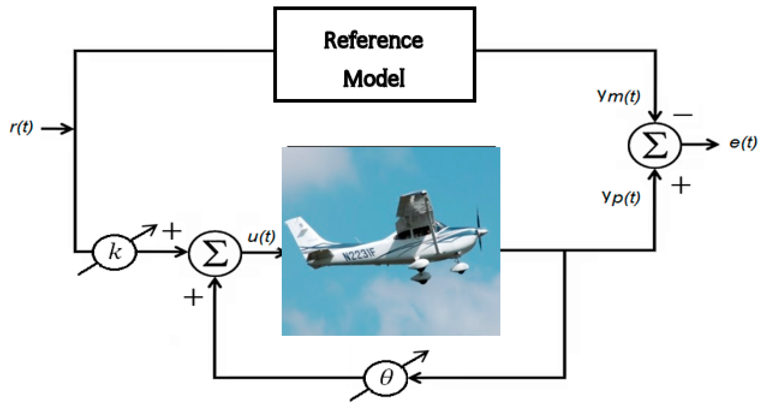
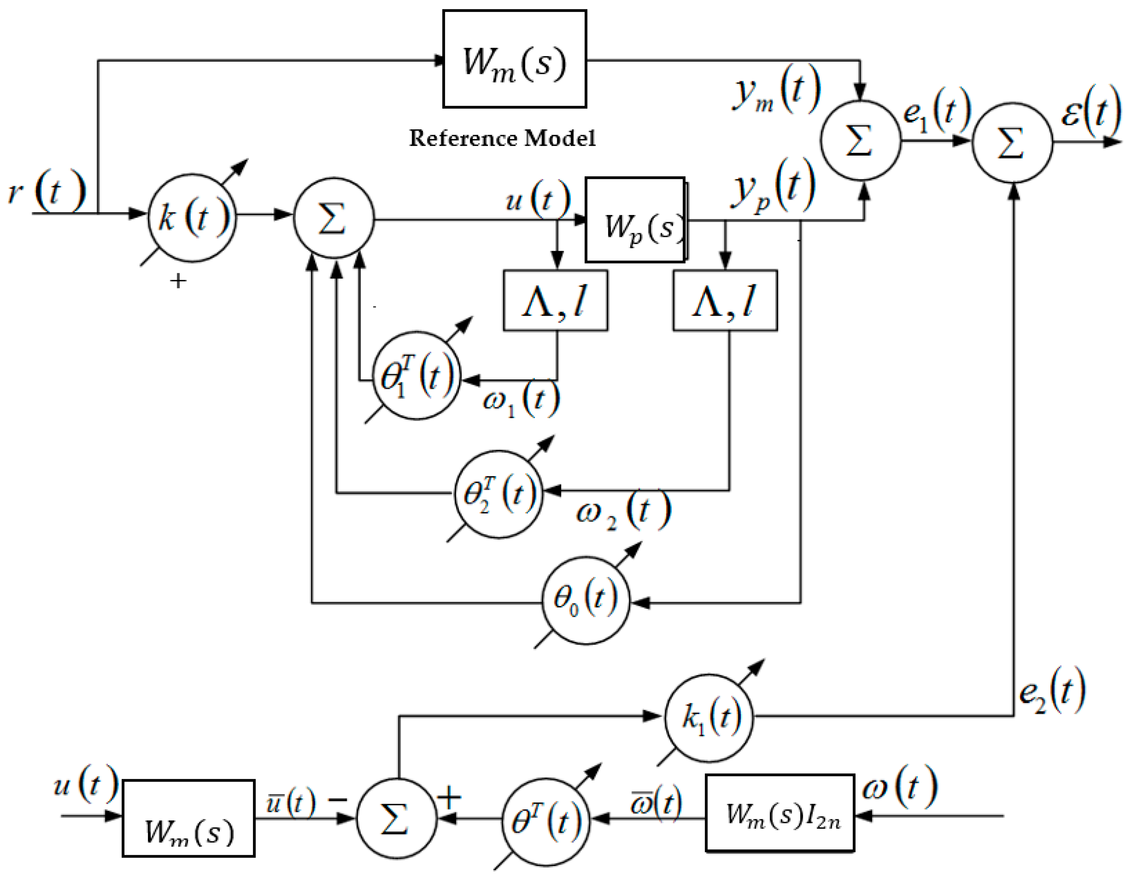
2.2. Control Process Description

Figure 2 shows a simplified schematic block diagram for the DMRAC, in which parameters $k$ and $\theta$ are adjusted over time for using their corresponding adaptive laws to maintain the error to be small or zero as t approaches infinity.

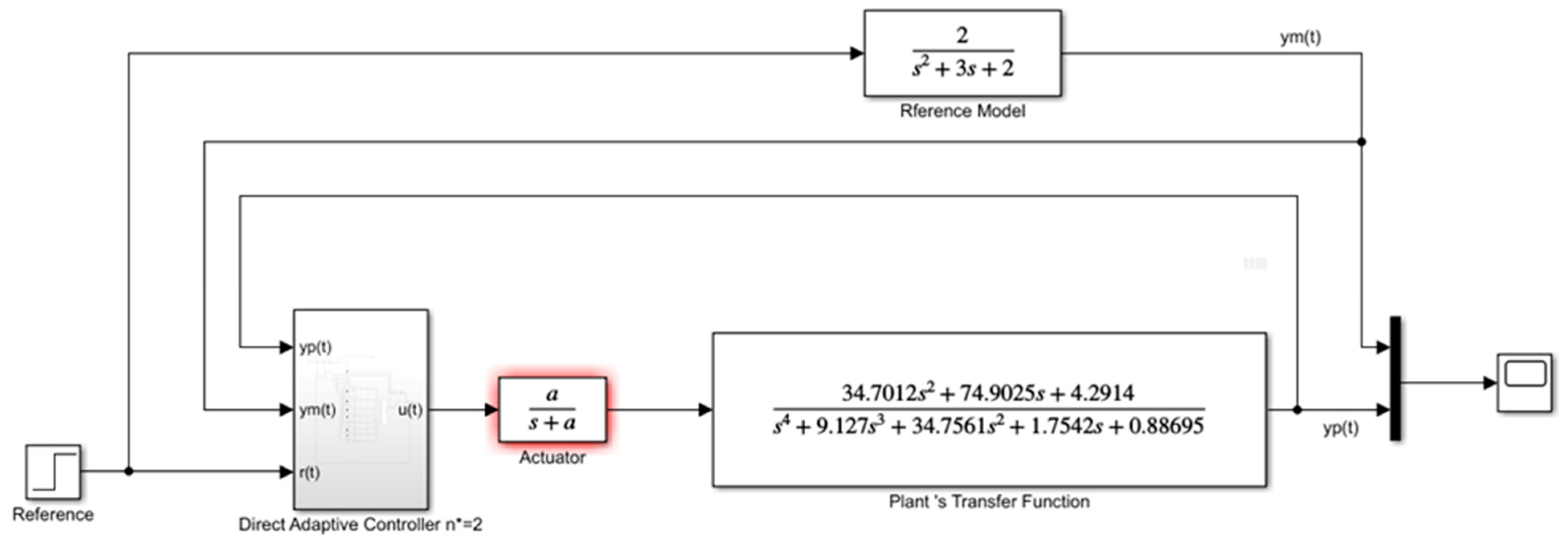
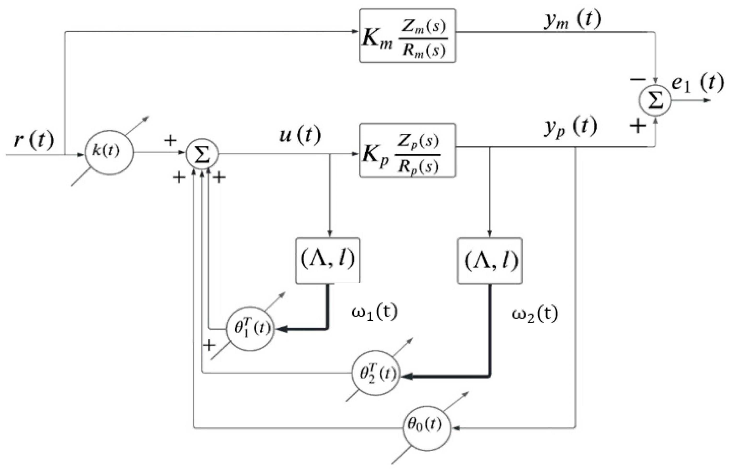
In our case, Figure 3 shows in detail the simplified block diagram of the DMRAC which will be used in this study, from analytical and simulation viewpoints. This Figure shows the plant, the reference model, the actuator, and the controller for the relative degree 2 ($n^{*}=2$). A complete block diagram implementation of the controller can be seen in [25].

For simplicity, we will consider that the actuator dynamic is fast enough for considering this transfer function as a unity (the same assumption is made for the sensor dynamic which is not shown in the block diagram).

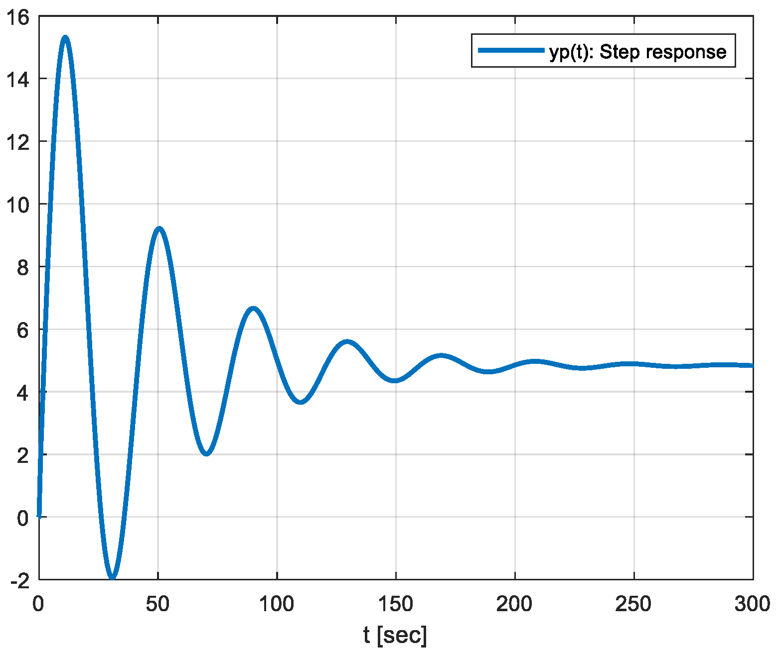
It is also interesting to show the behavior of the system output $y_p\left(t\right)=\theta \left(t\right)$, when the model reference output, denoted as $y_m\left(t\right)={\theta }_m\left(t\right),$ changes over time. Figure 4 shows the evolution of the system output $y_p\left(t\right)$ in open-loop when the input ${\delta }_e\left(t\right)$ is a unit step at t = 0.

From Figure 4 we can deduce that for any step change in the reference, the pilot should constantly manipulate the plane for almost 200 s to maintain a straight and level flight, which is a demanding task besides the navigation activities, and this motivates the development of automatic control strategies to help pilot duties.

3. Control Strategies

For the sake of completeness, a brief description of the DMRAC algorithm for plants of relative degree 2 $\left(n^{*}=2\right)$ (that will be used to control the plane as an alternative), is given in what follows. For a more detailed explanation of the algorithm, the reader is referred to [25].

DMRAC Algorithm

Generally speaking, the main objective of the MRAC is to minimize the error between the plant output and the model reference output. In the DMRAC, the controller parameter adjustment is based on the control error (difference between the actual and the desired outputs) [25].

For the particular case of the adaptive control of a linear (or linearized) nth order plant with a relative degree 1 $\left(n^{*}=1\right)$, it is used the DMRAC scheme shown in Figure 5, that gives rise to the well-known Error Model 1.

Under very well-known hypotheses [25], the control law for the DMRAC shown in Figure 5 has the form

$$u\left(t\right)={\theta }^T\left(t\right)·\omega \left(t\right),$$

where $\theta \left(t\right)={\left[k\left(t\right),{\theta }_1^T\left(t\right),{\theta }_0\left(t\right),{\theta }_2^T\left(t\right)\right]}^T\in {\mathfrak{R}}^{2n}$ and $\omega \left(t\right)={\left[r\left(t\right),{\omega }_1^T\left(t\right),y_p\left(t\right),{\omega }_2^T\left(t\right)\right]}^T\in {\mathfrak{R}}^{2n}$ are the controller parameters vector and the auxiliary signals vector, respectively, and $n$ is the order of the plant. The auxiliary signals ${\omega }_1∊R^{n-1},{\omega }_2∊R^{n-1}$ are defined by

$$\begin{gathered} {\dot{\omega }}_1\left(t\right)=\mathsf{\Lambda }{\omega }_1+lu\left(t\right), \\ {\dot{\omega }}_2\left(t\right)=\mathsf{\Lambda }{\omega }_2+ly\left(t\right), \end{gathered}$$

with ${k\left(t\right),}^{}{\theta }_0\left(t\right),r\left(t\right),y_p\left(t\right)\in {\mathfrak{R}}^{}$ and ${\theta }_1(t),{\theta }_2(t),{\omega }_1(t),{\omega }_2(t)\in {\Re }^{n-1}$. $(\mathsf{\Lambda },l)$ is any arbitrary stable and controllable pair, with $\mathsf{\Lambda }\in {\Re }^{n-1\times n-1}$ as an asymptotically stable matrix. For simplicity, in our study, we choose $(\mathsf{\Lambda },l)$ in the controllable canonical form. In this particular case $(n^{*}=1)$, the parameters adaptive laws are chosen as:

$$\begin{gathered} \dot{k}\left(t\right)=-sgn\left(k_p\right)e_1\left(t\right)r\left(t\right), \\ {\dot{\theta }}_0\left(t\right)=-sgn\left(k_p\right)e_1\left(t\right)y_p\left(t\right), \\ {\dot{\theta }}_1\left(t\right)=-sgn\left(k_p\right)e_1\left(t\right){\omega }_1\left(t\right), \\ {\dot{\theta }}_2\left(t\right)=-sgn\left(k_p\right)e_1\left(t\right){\omega }_2\left(t\right), \end{gathered}$$

(9)

and the output error $e_1\left(t\right)=y_p\left(t\right)-y_m\left(t\right)$ can be expressed as $e_1(t)=\frac{k_p}{k_m}{W}_m(s){\varphi }^T(t)\omega (t)$, where $W_m\left(s\right)$ is a strictly positive real (SPR) transfer function and $\varphi \left(t\right)=\theta \left(t\right)-{\theta }^{*}$ is the parametric error, with ${\theta }^{*}$ as the ideal (but unknown) control parameters.

$$\begin{array}{cc}\hfill \epsilon \left(t\right)& =e_1\left(t\right)+k\left(t\right)e_2\left(t\right)\hfill \\ e_2\left(t\right)\hfill & ={\theta }^T\left(t\right)\overline{\omega }\left(t\right)-W_m(s){\theta }^T\left(t\right)\omega (t)\hfill \\ \hfill \overline{\omega }\left(t\right)& =W_m(s)I_{2n}\omega (t)\hfill \end{array}$$

where $e_1\left(t\right)=y_p\left(t\right)-y_m\left(t\right)$ is the control error, $\epsilon \left(t\right)$ is the augmented control error, $e_2\left(t\right)$ is the auxiliary error, $\overline{\omega }\left(t\right)$ is a filtered version of $\omega \left(t\right)$ vector, and $k_1\left(t\right)$ is an additional adjustable parameter. $I_{2n}$ denotes the identity matrix of dimension $2n$.

In our specific case study, since the plant’s relative degree exactly equals 2 $(n^{*}=2)$, we can make a small modification to the diagram, as shown in Figure 5, (which is only valid for $n^{*}=1$), avoiding the introduction of the concept of augmented control error $\epsilon \left(t\right)$ and auxiliary error $e_2\left(t\right),$ simplifying the adaptive controller when $n^{*}$ is exactly 2. Figure 6 shows the modification introduced to the block diagram of Figure 5, with the new block in red.

For the particular case of the longitudinal movement of the airplane under investigation, we will use a fourth order model with a relative degree 2, but with making use of the simpler relative degree equal to 1 implementation, as shown in Figure 5, with the modification included in Figure 6.

Additionally, the corresponding simplified block diagram of Figure 6, for this specific case, the control error $e_1\left(t\right)$ can be expressed, as shown in Figure 7.

From Figure 7, the output error can be expressed as $e_1(t)=\frac{k_p}{k_m}{W}_m(s)L(s){\varphi }^T(t)\frac{\omega (t)}{L(s)}$ with $L\left(s\right)=\left(s+a\right)$, such that $W_m\left(s\right)L\left(s\right)$ is now an SPR Hurwitz transfer function and $\overline{\omega }\left(t\right)=\frac{\omega \left(t\right)}{L\left(s\right)}=\frac{\omega \left(t\right)}{s+a}$ is a new Hurwitz filtered version of $\omega \left(t\right)$. In this case, we can use adaptive laws similar to Equation (9) to change $\omega \left(t\right)$ by the filtered version $\overline{\omega }\left(t\right)$, that is to say

$$\begin{gathered} \dot{k}\left(t\right)=-sgn\left(k_p\right)e_1\left(t\right)\overline{r}\left(t\right), \\ {\dot{\theta }}_0\left(t\right)=-sgn\left(k_p\right)e_1\left(t\right){\overline{y}}_p\left(t\right), \\ {\dot{\theta }}_1\left(t\right)=-sgn\left(k_p\right)e_1\left(t\right){\overline{\omega }}_1\left(t\right), \\ {\dot{\theta }}_2\left(t\right)=-sgn\left(k_p\right)e_1\left(t\right){\overline{\omega }}_2\left(t\right), \end{gathered}$$

(10)

or written in the compact form

$$\dot{\theta }\left(t\right)=-sgn\left(k_p\right)e_1\left(t\right)\overline{\omega }\left(t\right),$$

(11)

where $\overline{\omega }\left(t\right)=\frac{1}{s+a}\left[r\left(t\right)y_p\left(t\right){\omega }_1\left(t\right){\omega }_2\left(t\right)\right]$ and $e_1(t)=\frac{k_p}{k_m}{W}_m(s)L(s){\varphi }^T(t)\frac{\omega (t)}{L(s)}$.

Furthermore, the control law $u\left(t\right)={\theta }^T\left(t\right)\omega \left(t\right)+{\dot{\theta }}^T\left(t\right)\overline{\omega }\left(t\right)$ in view of (11) can be expressed as

$$u\left(t\right)={\theta }^T\left(t\right)\omega \left(t\right)-sgn\left(k_p\right)e_1\left(t\right){\overline{\omega }}^T\left(t\right)\overline{\omega }\left(t\right),$$

that does not contain the parameter derivative.

Then, choosing $L\left(s\right)=(s+a)$, the realization of $P_L\left(\theta \right)=L\left(s\right)\theta \left(t\right)L^{-1}\left(s\right)$ [26] is free of drifts, and the subsequent stability test of the modified system under control becomes the essence of the solution to the control problem when the relative degree of the plant is 2 $(n^{*}=2$). Prior to ending this section, it is interesting to show some properties of the linear operator $P_L\left(\theta \right)$ used in the new adjustment control law. It satisfies the following properties:

$$\begin{array}{cc}(i)\hspace{1em}\hfill & P_L\left({\theta }^T\right)=L\left(s\right){\theta }^T\left(t\right)L^{-1}\left(s\right)\hfill \\ (ii)\hspace{1em}\hfill & P_L\left({\theta }^{*}\right)={\theta }^{*} \mathrm{if} {\theta }^{*}is\; constant;\hfill \\ (iii)\hspace{1em}\hfill & P_L\left(\theta \right)-\theta =P_L\left(\varphi \right)-\varphi , \mathrm{where} \theta \left(t\right)={\theta }^{*}+\varphi \left(t\right)\hfill \end{array}$$

4. Fractional Calculus Overview

In this section, we present some definitions and concepts on the derivative and integral operators of the fractional order [26,27] that will be used in the stability analysis of the implementation of the FO-DMRAC for flight control.

Definition 1 ([27]).

The Riemann–Liouville fractional integral of order $\alpha >0$ of a function $f\left(t\right)\in \mathbb{R}$ is defined by

$$I_{t_0}^{\alpha }f\left(t\right)=\frac{1}{\Gamma \left(\alpha \right)}{\int }_{t_0}^t\frac{f\left(\tau \right)}{(t-\tau {)}^{1-\alpha }}d\tau , t>t_0 \mathit{and} \mathcal{R}e\left(\alpha \right)>0,$$

(12)

where $\Gamma \left(\alpha \right)$ is the Gamma function defined as

$$\Gamma \left(\alpha \right)={\int }_0^{\infty }{t}^{\alpha -1}{e}^{-t}dt.$$

(13)

Definition 2 ([27]).

Let $\alpha \ge 0$ and $\left[n\right]=\alpha$. The Caputo fractional derivative of order $\alpha$ of a function $f\left(t\right)\in \mathbb{R}$ is defined as

$${}_{t_0}{}^C{D}_t^{\alpha }f\left(t\right)=\frac{1}{\Gamma \left(n-\alpha \right)}{\int }_{t_0}^t\frac{f^{\left(n\right)}\left(\tau \right)}{(t-\tau {)}^{\alpha -n+1}}d\tau ; {as long as f}^{\left(n\right)}\in L_1\left[t_0,t\right].$$

(14)

Some additional tools (lemmas and theorems) that are useful in the stability analysis of the fractional order adaptive control systems are presented in what follows.

Lemma 1 (Principle of fractional comparison).

Let $e\left(t\right)\in {\mathbb{R}}^n$ be a vector of differentiable functions. Then, $\forall t\ge t_0,$ the following inequality holds [28,29,30,31]

$${}_{t_0}{}^C{D}_t^{\alpha }\left\{e^T\left(t\right)Pe\left(t\right)\right\}\le 2e^T\left(t\right)P{}_{t_0}{}^C{D}_t^{\alpha }e\left(t\right), \forall \alpha \in \left(\mathrm{0,1}\right],$$

where $P\in {\mathbb{R}}^{n\times n}$ is a symmetric square matrix of constant coefficients and positive definite. A proof of Lemma 1 can be found in [28].

Another lemma that is useful in the study of the evolution of the output error in FO models is the following:

Lemma 2.

Let $e\left(·\right):{\mathbb{R}}^{+}\to \mathbb{R}$ be a uniformly continuous and bounded function. If there exists an $\alpha \in \left(\mathrm{0,1}\right],$ such that

$$\frac{1}{\Gamma \left(\alpha \right)}{\int }_{t_0}^t\frac{{e\left(\tau \right)}^2}{{\left(t-\tau \right)}^{1-\alpha }}d\tau <M, \forall t\ge t_0, \mathrm{with} M\in \left(0,\infty \right),$$

then

$$\underset{t\to \infty }{\lim }\left[t^{\alpha -\epsilon }\frac{{\int }_{t_0}^t{e\left(\tau \right)}^{2}d\tau }{t}\right]=0, \forall \epsilon >0.$$

A proof of this lemma is given in [30].

For completeness, we state Theorem 1 related to the boundedness and convergence of FO dynamical systems.

Theorem 1.

Let the state error $e\left(t\right)$ and the output error $e_1\left(t\right)$ be represented by equations

$$\begin{array}{cc}{}_{t_0}{}^C{D}_t^{\beta }e\left(t\right)=A_{mn}e\left(t\right)+b_{mn}\left[{\varphi }^T\left(t\right)\omega \left(t\right)\right],\hspace{1em}\hfill & \hfill e\left(t_0\right)=e_0,\\ e_1\left(t\right)=k_p{h}_{mn}^{T}e\left(t\right),\hfill & \hfill e_1\left(t_0\right)=e_{10},\end{array}$$

(15)

where $A_{mn}\in {\mathbb{R}}^{n\times n}$ is a Hurwitz matrix and such that given matrix $Q=Q^T>0\in {\mathbb{R}}^{n\times n}$. Then, there exists a matrix $P=P^T>0\in {\mathbb{R}}^{n\times n},$ such that

$$\begin{gathered} A_{mn}^{T}P+P{A}_{mn}=-Q, \\ P{b}_{mn}=h_{mn}{k}_p \end{gathered}$$

This implies that the triplet $\left\{A_{mn},b_{mn},h_{mn}\right\}$ satisfies the conditions of the Kalman–Yakubovich–Popov Lemma [25]. Furthermore, $k_p$ is an unknown constant, but with a known sign, $e\left(t\right):{\mathbb{R}}^{+}\to {\mathbb{R}}^n$ corresponds to the vector of the non-accessible states error, $e_1\left(t\right):{\mathbb{R}}^{+}\to \mathbb{R}$ is the output error (accessible), $b_{mn},h_{mn}\in {\mathbb{R}}^n$ with $\varphi \left(t\right):{\mathbb{R}}^{+}\to {\mathbb{R}}^m$ is the parameter error vector defined as $\varphi \left(t\right)=\theta \left(t\right)-{\theta }^{*}$ with $\theta \left(t\right):{\mathbb{R}}^{+}\to {\mathbb{R}}^m,$ the estimated parameters (of the controller) and ${\theta }^{*}:{\mathbb{R}}^{+}\to {\mathbb{R}}^m,$ the unknown ideal parameters (of the controller). $\omega \left(t\right):{\mathbb{R}}^{+}\to {\mathbb{R}}^m$ is a vector of available auxiliary signals and $\beta \in \left(\mathrm{0,1}\right]$ is the fractional order of the plant, whose adaptive adjustment laws estimate the unknown controller parameters, which are given by

$${}_{t_0}{}^C{D}_t^{\alpha }\varphi \left(t\right)={}_{t_0}{}^C{D}_t^{\alpha }\theta \left(t\right)=-\gamma sgn\left(k\right)e_1\left(t\right)\omega \left(t\right),\hspace{1em}\varphi \left(t_0\right)=0$$

(16)

with $\alpha <\beta$ and $\alpha \in \left(\mathrm{0,1}\right]$. Then, assuming that $e\left(t\right)$ and $\varphi \left(t\right)$ are differentiable and uniformly continuous functions, it holds that

• The parametric error $\varphi \left(t\right)$, the state error $e\left(t\right),$ and the output error $e_1\left(t\right)$ remain bounded for all time;
• Furthermore, if the auxiliary signal $\omega \left(t\right)$ is bounded, then ${}_{t_0}{}^C{D}_t^{\alpha }\varphi \left(t\right)$ and ${}_{t_0}{}^C{D}_t^{\beta }e\left(t\right)$ also remain bounded;
• The mean value of the squared norm of the state error $\overline{{‖e\left(t\right)‖}^2}$ is $\left(t^{\epsilon -\alpha }\right)$ $\forall \epsilon >0$.
  The proof of this theorem can be found in [32].

Corollary 1.

From Theorem 1, it is evident that if (iii) holds, it must also hold that the mean value of the square norm of the output error $e_1\left(t\right)$ is $\left(t^{\epsilon -\alpha }\right)$$\forall \epsilon >0$, since $e_1\left(t\right)=h_{mn}^{T}e\left(t\right)$ with $h_{mn}^T$ a vector has components that are constants.

Finally, a new lemma (Lemma 3) for the case when the relative degree is 2 $(n^{*}=2)$ is stated, that relaxes the hypothesis made on the auxiliary signals $\omega \left(t\right)$ in point (ii) of Theorem 1.

Lemma 3.

Let us consider a system of order $n$ and relative degree $n^{*}=2$ represented by the state equations

$$\begin{gathered} {\dot{x}}_p\left(t\right)=A_p{x}_p\left(t\right)+b_{p}u\left(t\right), \\ {y}_p\left(t\right)=h_p^T{x}_p\left(t\right), \end{gathered}$$

(17)

whose FO adaptive laws to adjust the controller parameters are given by

$${}_{t_0}{}^C{D}_t^{\alpha }\varphi \left(t\right)={}_{t_0}{}^C{D}_t^{\alpha }\theta \left(t\right)=-\gamma e_1\left(t\right)\overline{\omega }\left(t\right),\hspace{1em}\varphi \left(t_0\right)=0,$$

and whose error equation is given by (in this case, the error equation is of integer order, that is to say, $\beta =1$ with $\beta >\alpha$. See Equation (15),

$$\begin{array}{cc}\dot{e}\left(t\right)=A_{mn}e\left(t\right)+b_{rp}[\varphi \left(t\right)\overline{\omega }\left(t\right)],\hspace{1em}\hfill & \hfill e\left(t_0\right)=e_0,\\ e_1\left(t\right)=h_{mn}^{T}e\left(t\right),\hfill & \hfill e_1\left(t_0\right)=e_{10},\end{array}$$

(18)

$A_p\in {\mathbb{R}}^{n\times n}$ is the state matrix of the plant, $x_p\in {\mathbb{R}}^n$ is the state vector, $b_p$ and $h_p$ are vectors $\in {\mathbb{R}}^n$ whose input $u\left(t\right)$ and output are $y_p\left(t\right)\in \mathbb{R}$, such that $Z_p\left(s\right)$ and $R_p\left(s\right)$ are monic polynomials of order $n-2$ and n, respectively. $k_p$ is s constant parameter called the high frequency gain, and its sign is known. Without a loss of generality, we will consider that it is positive throughout the entire analysis, and ($k_p>0$) and $Z_p\left(s\right)$ is Hurwitz. In addition, it is assumed that the parameters of the plant (gain $k_p$ and coefficients of the polynomials $Z_p\left(s\right)$ and $R_p\left(s\right)$) are unknown and their reference model is also of the relative degree 2 ($n_m^{*}=2$) and Hurwitz, where $A_{mn}$ is also Hurwitz. Then, since $e\left(t\right)$ and $\varphi \left(t\right)$ are bounded by part (i) of Theorem 1, the auxiliary signals $\omega \left(t\right)$ and $\overline{\omega }\left(t\right)$ will also be bounded. This is an important conclusion because we do not need to assume that the auxiliary signals $\omega \left(t\right)$ or $\overline{\omega }\left(t\right)$ should be bounded, as is imposed in part (ii) of Theorem 1.

Proof. 

Assuming that $e\left(t\right)$ and $\varphi \left(t\right)$ are uniformly continuous and differentiable, and based on Theorem 1, in which it has been shown that both $e\left(t\right)$ and $\varphi \left(t\right)$ are bounded, then, $\dot{e}\left(t\right)$ will also be bounded, since $e\left(t\right)$ is bounded, differentiable, and uniformly continuous. Then, since the auxiliary signals $\omega \left(t\right)$ and $\overline{\omega }\left(t\right)$ are part of the equation for $\dot{e}\left(t\right)$ (Equation (18)), then $\omega \left(t\right)$ must be bounded and $\overline{\omega }\left(t\right)$ will also be bounded, since $\overline{\omega }\left(t\right)=\frac{1}{\left(s+a\right)}\omega \left(t\right)$ is with $\frac{1}{\left(s+a\right)}$ Hurwitz. This concludes the proof. □

In our case, the control law is $u\left(t\right)={\theta }^T\left(t\right)\omega \left(t\right)-sgn\left(k_p\right)e_1\left(t\right){\overline{\omega }}^T\left(t\right)\overline{\omega }\left(t\right),$ but it can also be the classical adaptive control law $u\left(t\right)={\theta }^T\left(t\right)\omega \left(t\right),$ as long as the structure of the error equation is of Equation (18) type, in which case, $\overline{\omega }\left(t\right)$ is replaced by $\omega \left(t\right)$.

Remark 1.

Lemma 3 can be easily extended to the general case when $n^{*}\ge 2,$ as long as$\beta$ of Equation (15) is equal to 1 $\left(\beta =1\right),$ as is the case of Equation (18).

This lemma allows us to relax the hypothesis that must be considered in Theorem 1, in order to prove that the FO derivatives are bounded, the auxiliary signal $\omega \left(t\right)$ should also be bounded, which is not necessary to impose in the case of $\beta =1$. In other cases, with $\beta \in \left(\mathrm{0,1}\right)$, only Theorem 1 should be used by now.

Furthermore, if the auxiliary signal $\omega \left(t\right)$ is bounded (as shown in Lemma 3), then Theorem 1 guarantees that the squared norm of the state error ${‖e\left(t\right)‖}^2$ and the output ${\left|e_1\left(t\right)\right|}^2$ tend to 0, as t tends to infinity. Thus, the stability of the proposed FO adaptive control system has been proved.

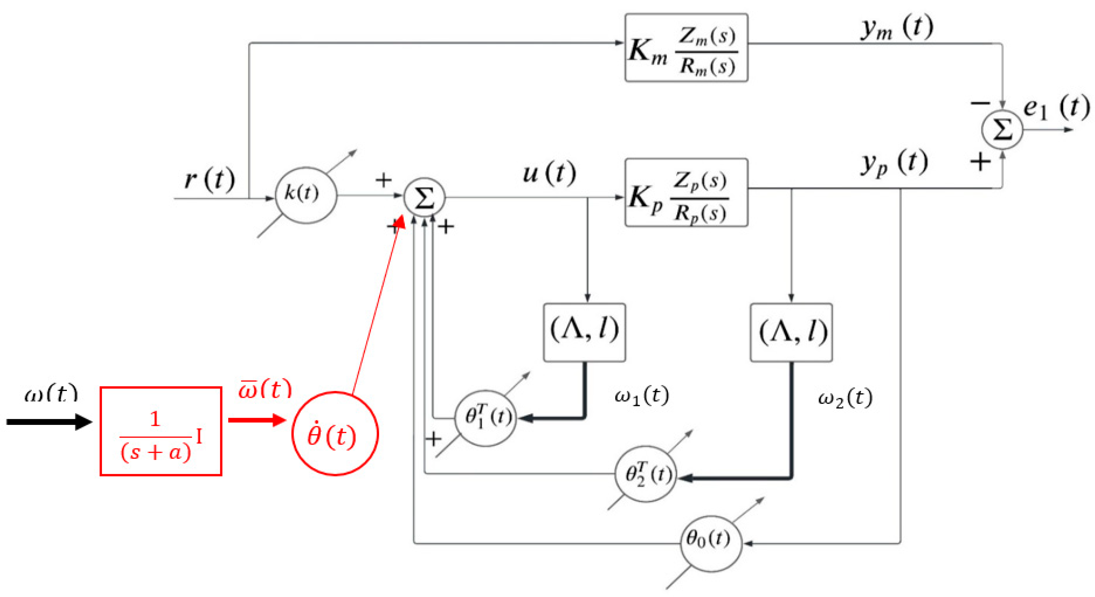
FO-DMRAC Algorithm

Figure 6 shows the block diagram of the FO-DMRAC for the specific case when $n^{*}=2$. Since the equation of the plant is of integer order, the only equations that change are the adaptive laws. For comparison purposes, it is interesting to note that for the IO case and $n^{*}=2$, these adaptive laws are given by

$$\dot{\theta }\left(t\right)=\dot{\varphi }\left(t\right)=-sgn\left(k_p\right)e_1\left(t\right)\overline{\omega }\left(t\right)$$

(19)

and for the FO case, these adaptive laws become

$${}_{t_0}{}^C{D}_t^{\alpha }\theta \left(t\right)={}_{t_0}{}^C{D}_t^{\alpha }\varphi \left(t\right)=-sgn(k_p)e_1\left(t\right)\overline{\omega }\left(t\right)$$

(20)

The control law in both cases is given by

$$u\left(t\right)={\theta }^T\left(t\right)\omega \left(t\right)-sgn\left(k_p\right)e_1\left(t\right){\overline{\omega }}^T\left(t\right)\overline{\omega }\left(t\right)$$

(21)

where $\overline{\omega }\left(t\right)=\frac{1}{\left(s+a\right)}\omega (t)$ with $a$, an arbitrary scalar is greater than 0. For simplicity, we will choose $a=1$. Furthermore, the high frequency gain of the plant is $k_p=34.7012$ (see Equation (7)), which is supposed to be unknown, but its sign is assumed to be known $\left(sgn\right(kp)>0)$.

5. Simulation Results and Comparisons

Computer simulations were performed in MATLAB-Simulink [33,34]. For all simulations, zero initial conditions were considered for the airplane.

Table 4. Implementation of the IO-DMRACs and FO-DMRACs.

Reference model	$W_m\left(s\right)=\frac{2}{s^2+3s+2}$
Plant	$W_p\left(s\right)=\frac{34.7012s^2+74.9025s+4.2914}{s^4+9.127s^3+34.7561s^2+1.7542s+0.8695}$
Control laws	$\theta \left(t\right)={\left[\begin{array}{cccc}k\left(t\right)& {\theta }_1^T\left(t\right)& {\theta }_0\left(t\right)& {\theta }_2^T\left(t\right)\end{array}\right]}^T\in {\mathbb{R}}^8$ $\omega \left(t\right)={\left[\begin{array}{cccc}r\left(t\right)& {\omega }_1^T\left(t\right)& y_p\left(t\right)& {\omega }_2^T\left(t\right)\end{array}\right]}^T\in {\mathbb{R}}^8$ $u\left(t\right)={\theta }^T\left(t\right)\omega \left(t\right)-e_1\left(t\right){\overline{\omega }}^T\left(t\right)\overline{\omega }\left(t\right)$ Note: ${\theta }_1^T\left(t\right)$ and ${\theta }_2^T\left(t\right)$ $\in {\mathbb{R}}^3$
Auxiliary signals	${\dot{\omega }}_1\left(t\right)=\mathsf{\Lambda }{\omega }_1\left(t\right)+lu\left(t\right)$ ${\dot{\omega }}_2\left(t\right)=\mathsf{\Lambda }{\omega }_2\left(t\right)+l{y}_p\left(t\right)$ $\mathsf{\Lambda }=\left[\begin{array}{ccc}0& 1& 0\\ 0& 0& 1\\ -6& -11& -6\end{array}\right]$ $l={\left[0 0 1\right]}^T$
First order filter L(s) with a = 1.	$L\left(s\right)=\frac{1}{\left(s+a\right)}=\frac{1}{\left(s+1\right)}$
Output error	$e_1\left(t\right)=\frac{k_p}{k_m}{\overline{W}}_m\left(s\right){\varphi }^T\left(t\right)\overline{\omega }\left(t\right)$ ${\overline{W}}_m\left(s\right)=\left(s+1\right)W_m\left(s\right)$ y $\overline{\omega }\left(t\right)=\frac{1}{\left(s+1\right)}\omega \left(t\right)$
Integer order adaptive laws	$\dot{\theta }\left(t\right)=-\gamma e_1\left(t\right)\overline{\omega }\left(t\right)$
Fractional order adaptive laws	${}_{t_0}{}^C{D}_t^{\alpha }\theta \left(t\right)=-\gamma e_1\left(t\right)\overline{\omega }\left(t\right)$

shows the implementation details of the IO-DMRACs and the FO-DMRACs.

Fractional adaptive laws were implemented using the Ninteger Toolbox for MATLAB [35]. Specifically, the NID block was used, which is based on the Oustaloup approximation method [36]. In this study, five poles and five zeros were selected in the implementation, and the frequency interval chosen was $\omega \in [0.01;$ 100] [rad/s]. It is important to mention that better approximations can be achieved if the bandwidth is increased (e.g., $\in [0.010; 1000]$ at the expense of increasing the simulation time.

5.1. IO-DMRAC v/s FO-DMRAC Using the Particle Swarm Optimization (PSO)

In this Section, we compare the control results using IO-DMRAC v/s FO-DMRAC, when the controller parameters of both implementations are optimized using the particle swarm optimization (PSO) technique [22,37], using 50 particles and 50 iterations. It should be noted that any other optimization technique could also be used to determine the controller’s parameters, and it is at the discretion of the designer. First, we analyze the open-loop response of the plant to a unit step input and zero initial conditions to observe the behavior of the oscillations during the transient period before reaching the steady-state regime. 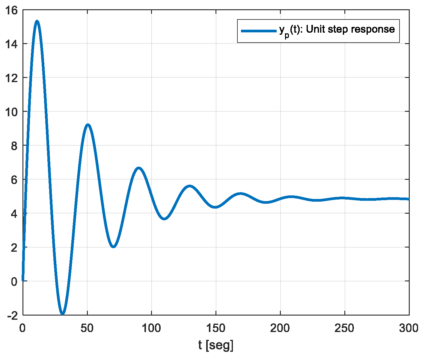The result is shown in Figure 8.

From the open-loop response shown in Figure 8, we note that the time to reach the steady state regime is almost 300 s, which is considered too long. Therefore, an automatic control system has to be designed to reduce the time of the transient response while tracking the reference accurately.

5.2. Simulation Results Using the Exact Knowledge of $n^{*}=2$

In this section, we analyze the behavior of the controller given in Figure 6, i.e., assuming that the relative degree of the plant is exactly equal to 2.

The objective function used to optimize the process behavior is defined as

$$J_{norm}={\omega }_{ess}{e}_{ss}+{\omega }_{du}{\int }_{t_0=0}^t\left|\frac{du}{dt}\right|dt+{\int }_{t_0=0}^t\left({\omega }_e·\frac{e_1^2\left(t\right)}{{\sigma }_e\left(t\right)}+{\omega }_u·\frac{u^2\left(t\right)}{{\sigma }_u\left(t\right)}\right)dt$$

(22)

where $e_{ss}$ is the control steady-state error, $\left|\frac{du}{dt}\right|$ is the rate of change of the input to the plant (or the controller output), $e_1\left(t\right)$ is the control error, $\left(t\right)$ is the output of the controller, ${\omega }_e$ and ${\omega }_u$ are the weighted parameters, and ${\sigma }_e\left(t\right)$ and ${\sigma }_u\left(t\right)$ are the standard deviations of the control error and controller output as a time function, respectively. The reference is the unit step.

Remark 2.

In this study, a rather general objective function (Equation (22)) was chosen. Nevertheless, any other properly defined objective function could also be used by the designer.

Using the values and equations shown in Table 4 and considering the weights ${\omega }_{ess}=1$, ${\omega }_{du}=1$, ${\omega }_e=2,$ and ${\omega }_u=1$, the design parameter values for each case (IO-DMRAC and FO-DMRAC) were obtained and used in the simulations.

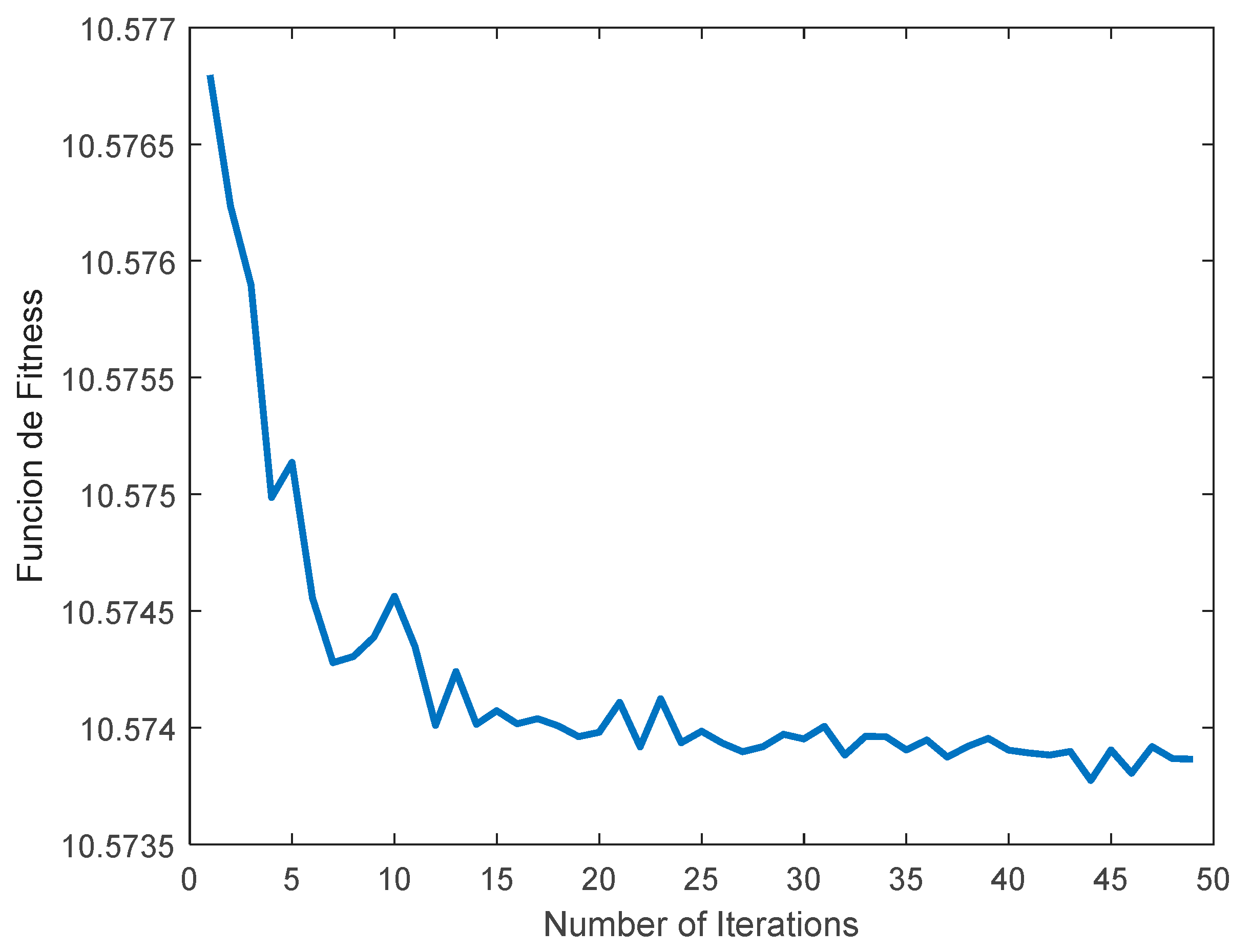
Figure 9 shows the evolution of the fitness function (objective function) $J_{norm}$ as a function of the number of iterations used in the PSO algorithm.

The optimal parameter values obtained for the case of IO-DMRAC were:

$$\begin{gathered} {\gamma }_k=5.3633, {\gamma }_{11}=0.1, {\gamma }_{12}=0.1, {\gamma }_{13}=49.58, \\ {\gamma }_0=0.1, {\gamma }_{21}=0.1, {\gamma }_{22}=7.6837 \mathrm{and} {\gamma }_{23}=0.1. \end{gathered}$$

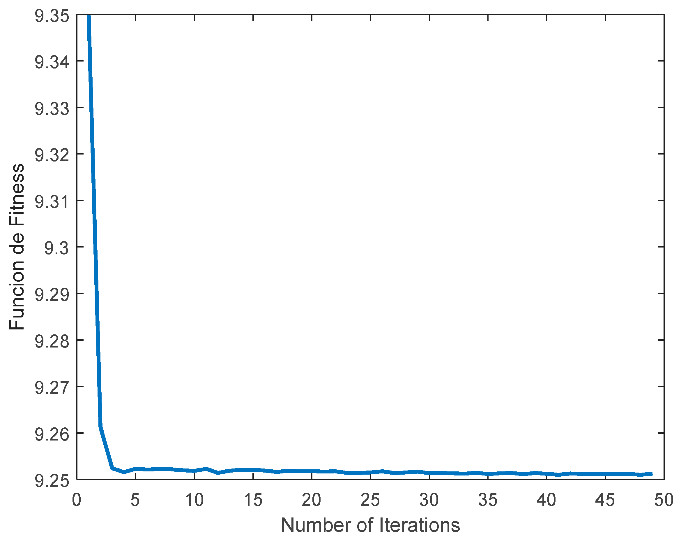
As in the previous case, Figure 10 shows the evolution of the objective or fitness function while increasing the number of iterations of the PSO method in the case of the FO-DMRAC.

The best parameter values obtained for the FO-DMRAC case were

$$\begin{gathered} {\alpha }_k=0.3, {\alpha }_{11}=0.5315, {\alpha }_{12}=1, {\alpha }_{13}=1, \\ {\alpha }_0=0.3, {\alpha }_{21}=0.3, {\alpha }_{22}=1, {\alpha }_{23}=0.8608, \\ {\gamma }_k=5.6173, {\gamma }_{11}=0.03, {\gamma }_{12}=0.03, {\gamma }_{13}=33.5375, \\ {\gamma }_0=0.03, {\gamma }_{21}=10.0493, {\gamma }_{22}=0.03, {\gamma }_{23}=0.11957. \end{gathered}$$

From Figure 9 and Figure 10, it is interesting to observe a faster rate of convergence to a stable value of the objective function in the FO case (Figure 10) compared to the integer case (Figure 9), even though the number of optimization parameters is twice the one used in the IO case. This seems to be an indication that, since in the FO case there are more degrees of freedom in the controller, the behavior attained is better than the one obtained for the IO case.

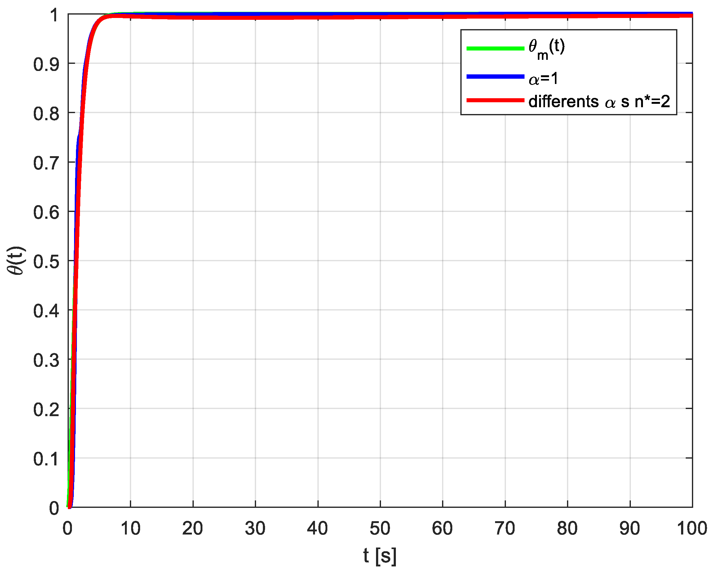
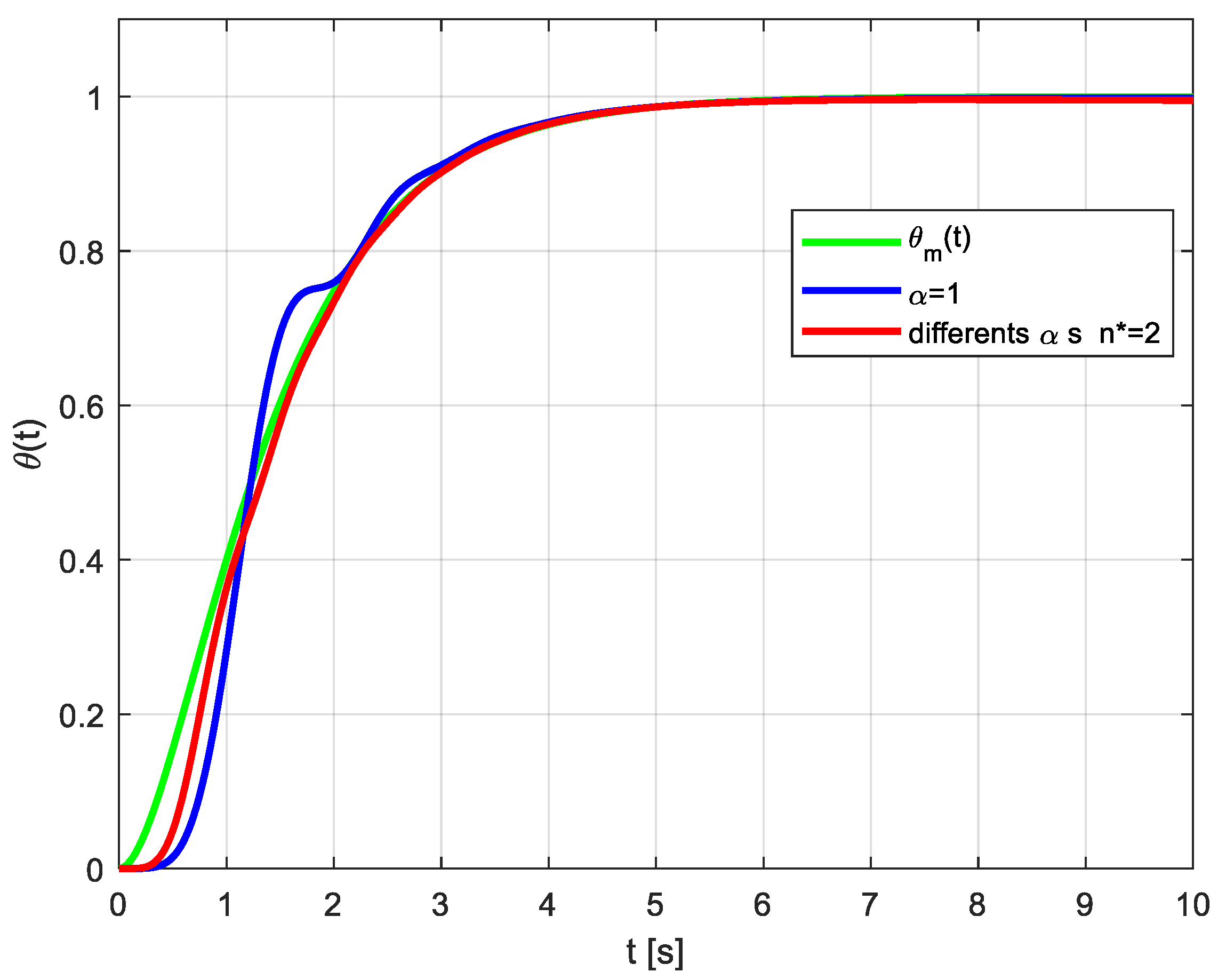
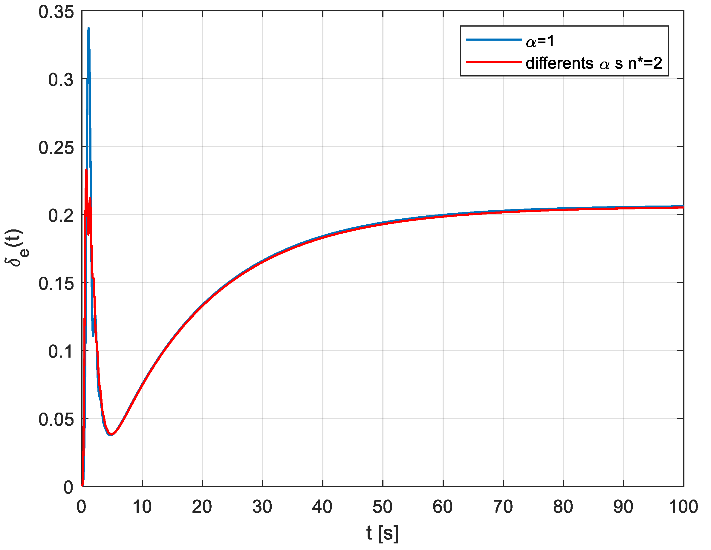
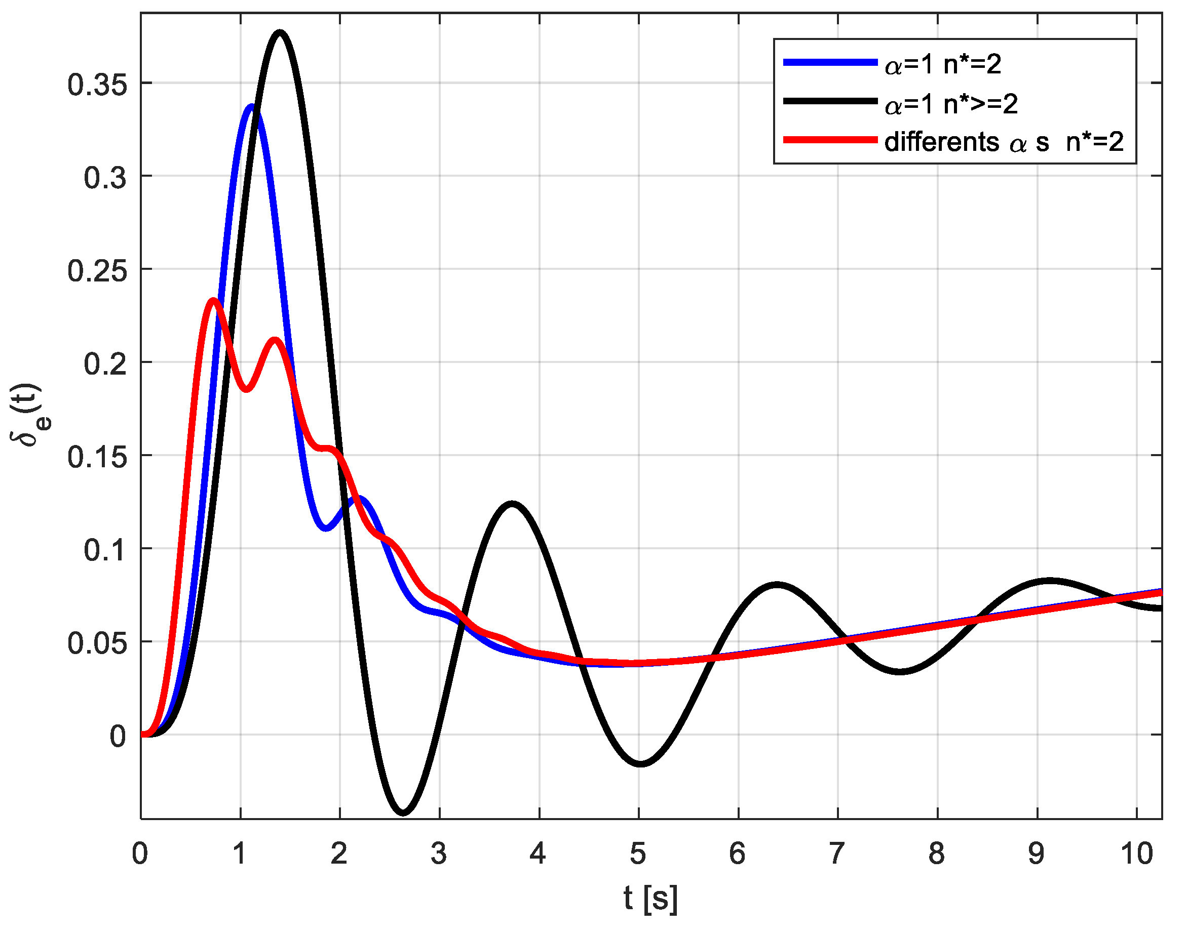
Figure 11 and Figure 12 show the responses of both adaptive controllers regarding the tracking of the reference signal (in green). Both responses are similar to FO-DMRAC and IO-DMRAC and approximate the reference very well. Nevertheless, in the case of FO-DMRAC, the response is smoother than in the IO-DMRAC case.

Moreover, Figure 13 and Figure 14 show that the control effort in the IO case is greater than that required in the FO case. Particularly, this effort for the IO case is greater in the transient period.

Table 5. $J_{norm}$ cost function using optimization by PSO for IO-DMRAC and FO-DMRAC.

	ISE	ISI	$\mathit{I}\mathit{S}\mathit{E}+\mathit{I}\mathit{S}\mathit{I}$	${\mathit{J}}_{\mathit{n}\mathit{o}\mathit{r}\mathit{m}}$
IO-DMRAC-PSO	0.0207	3.056	3.0767	10.31
FO-DMRAC-PSO	0.0090	3.005	3.014	8.989

shows the optimal values of the cost function $J_{norm}$ when all controller parameters are varied.

From Table 5, it can be seen that a better performance is achieved when using FO-DMRAC, since all of the indices are smaller than the IO case. Furthermore, the control effort is smaller in the transient period, as is shown in Figure 14.

Remember that the weights used in the optimization processes were chosen as ${\omega }_{ess}=1$, ${\omega }_{du}=1$, ${\omega }_e=2,$ and ${\omega }_u=1$.

5.3. Simulation Results Using the Generalized Controller for $n^{*}\ge 2$

In this section, we analyze the problem from a viewpoint different from the one used in Section 5.1, i.e., using the general implementation of the FO-DMRAC when the relative degree is greater than or equal to 2 ($n^{\mathrm{*}}\ge 2$). The idea is to compare the behavior with the one implemented in Section 5.1, which, as mentioned, only works for the case when the relative degree is exactly equal to 2 ($n^{\mathrm{*}}=2$).

The block diagram of the generalized DMRAC when $n^{\mathrm{*}}\ge 2$ is shown in Figure 15 [25]. In this case, additional errors must be considered, such as the auxiliary error $e_2\left(t\right)$ and augmented error $\epsilon \left(t\right)$, as well as an additional gain $k_1\left(t\right)$. In this case, $W_m\left(s\right)$ and $W_p\left(s\right)$ are the transfer functions of the reference model and the plant, respectively.

It is important to mention that the structure of Figure 15 is the same for both the integer and fractional adaptive control cases. The only difference lies in the laws for the adjustment of the parameters (IO derivative in one case and FO derivative in the other one).

Then, to make the analysis comparable (when $n^{*}=2$ and FO-DMRAC) with the generalized adaptive implementation of the integer order DMRAC (or IO-DMRAC), we have determined the values of the γ’s and α’s optimized by PSO. The resulting values are:

$$\begin{gathered} {\gamma }_k=5.3633, {\gamma }_{11}=0.1, {\gamma }_{12}=0.1, {\gamma }_{13}=49.58, \\ {\gamma }_0=0.1, {\gamma }_{21}=0.1, {\gamma }_{22}=7.6837, {\gamma }_{23}=0.1. \end{gathered}$$

Table 6. Implementation details of the general IO-DMRAC controller for the case $n^{*}\ge 2$.

Reference Model	$W_m\left(s\right)=\frac{2}{s^2+3s+2}$
Plant	$W_p\left(s\right)=\frac{34.7012s^2+74.9025s+4.2914}{s^4+9.127s^3+34.7561s^2+1.7542s+0.8695}$
Generalized control law	$\theta \left(t\right)={\left[\begin{array}{cccc}k\left(t\right)& {\theta }_1^T\left(t\right)& {\theta }_0\left(t\right)& {\theta }_2^T\left(t\right)\end{array}\right]}^T\in {\mathbb{R}}^8$ $\omega \left(t\right)={\left[\begin{array}{cccc}r\left(t\right)& {\omega }_1^T\left(t\right)& y_p\left(t\right)& {\omega }_2^T\left(t\right)\end{array}\right]}^T\in {\mathbb{R}}^8$ $u\left(t\right)={\theta }^T\left(t\right)\omega \left(t\right)$
Auxiliary signals	${\dot{\omega }}_1\left(t\right)=\mathsf{\Lambda }{\omega }_1\left(t\right)+lu\left(t\right)$ ${\dot{\omega }}_2\left(t\right)=\mathsf{\Lambda }{\omega }_2\left(t\right)+l{y}_p\left(t\right)$ $\mathsf{\Lambda }=\left[\begin{array}{ccc}0& 1& 0\\ 0& 0& 1\\ -6& -11& -6\end{array}\right]$ $l={\left[0 0 1\right]}^T$ $\overline{u}\left(t\right)=W_m\left(s\right)u\left(t\right)$ $\overline{\omega }\left(t\right)=W_m\left(s\right)\omega \left(t\right)$
Output error and augmented error	$e_1\left(t\right)=y_P\left(t\right)-y_m\left(t\right)$ $e_2\left(t\right)={\theta }^T\left(t\right)\overline{\omega }\left(t\right)-\overline{u}\left(t\right)$ $\epsilon \left(t\right)=e_1\left(t\right)+k\left(t\right)e_2\left(t\right)$
Integer order adaptive laws	${\dot{k}}_1\left(t\right)=-\gamma \frac{\epsilon \left(t\right)e_2\left(t\right)}{1+\overline{\omega }\left(t\right){\overline{\omega }}^T\left(t\right)}$ $\dot{\theta }\left(t\right)=-\gamma \frac{\epsilon \left(t\right)\overline{\omega }\left(t\right)}{1+\overline{\omega }\left(t\right){\overline{\omega }}^T\left(t\right)}$

shows the design parameters for the general case IO-DMRAC when the relative degree of the plant is greater than or equal to 2 ($n^{*}\ge 2$).

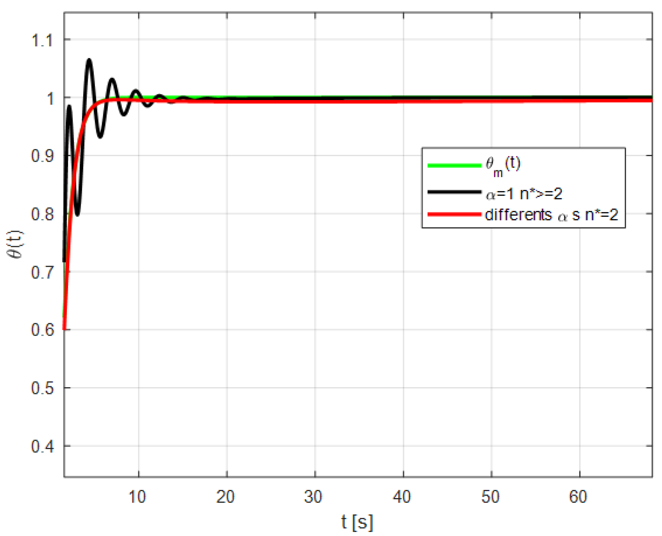
A plot of the pitch angle $\theta \left(t\right)$ for the generalized IO-DMRAC case ($n^{*}\ge 2;\mathrm{b}\mathrm{l}\mathrm{a}\mathrm{c}\mathrm{k} \mathrm{c}\mathrm{o}\mathrm{l}\mathrm{o}\mathrm{r}$) and FO-DMARC case ($n^{*}=2;\mathrm{r}\mathrm{e}\mathrm{d} \mathrm{c}\mathrm{o}\mathrm{l}\mathrm{o}\mathrm{r}$) are shown in Figure 16 together with the output signal of the reference model ${\theta }_m\left(t\right)$ in green.

${\theta }_m\left(t\right)$ is the reference signal or the desired evolution of the pitch angle (green color). The signal in black is the plant output when the generalized IO-DMRAC implementation is used (i.e., $n^{*}\ge 2$), and finally in red, the plant output is shown when FO-DMRAC is considered using the simple structure ($n^{*}=2$)

Without being exhaustive, it can be seen from Figure 16 and Figure 17 that the best response and least control effort is achieved with the FO-DMRAC for $n^{*}=2$. Furthermore, the generalized IO-DMRAC case presents oscillations in the transient period, something that does not occur in the cases of the IO and FO controls when $n^{*}=2$.

It is important to point out that the generalized case corresponds to the structure shown in Figure 15 (i.e., $n^{*}\ge 2)$. Furthermore, as discussed in the previous paragraph, the results for the generalized IO-DMRAC-PSO case are supported by the results shown in

Table 7. $J_{norm}$ cost function using PSO for IO-DMRAC and FO-DMRAC.

	$\mathit{I}\mathit{S}\mathit{E}+\mathit{I}\mathit{S}\mathit{I}$	${\mathit{J}}_{\mathit{n}\mathit{o}\mathit{r}\mathit{m}}$
IO-DMRAC-PSO	3.0767	10.31
FO-DMRAC-PSO	3.014	8.989
Generalized IO-DMRAC-PSO	3.29046	13.5

, where the best result is achieved with the FO-DMRAC with a relative degree exactly equal to 2 ($n^{*}=2$), and with text highlighted in blue.

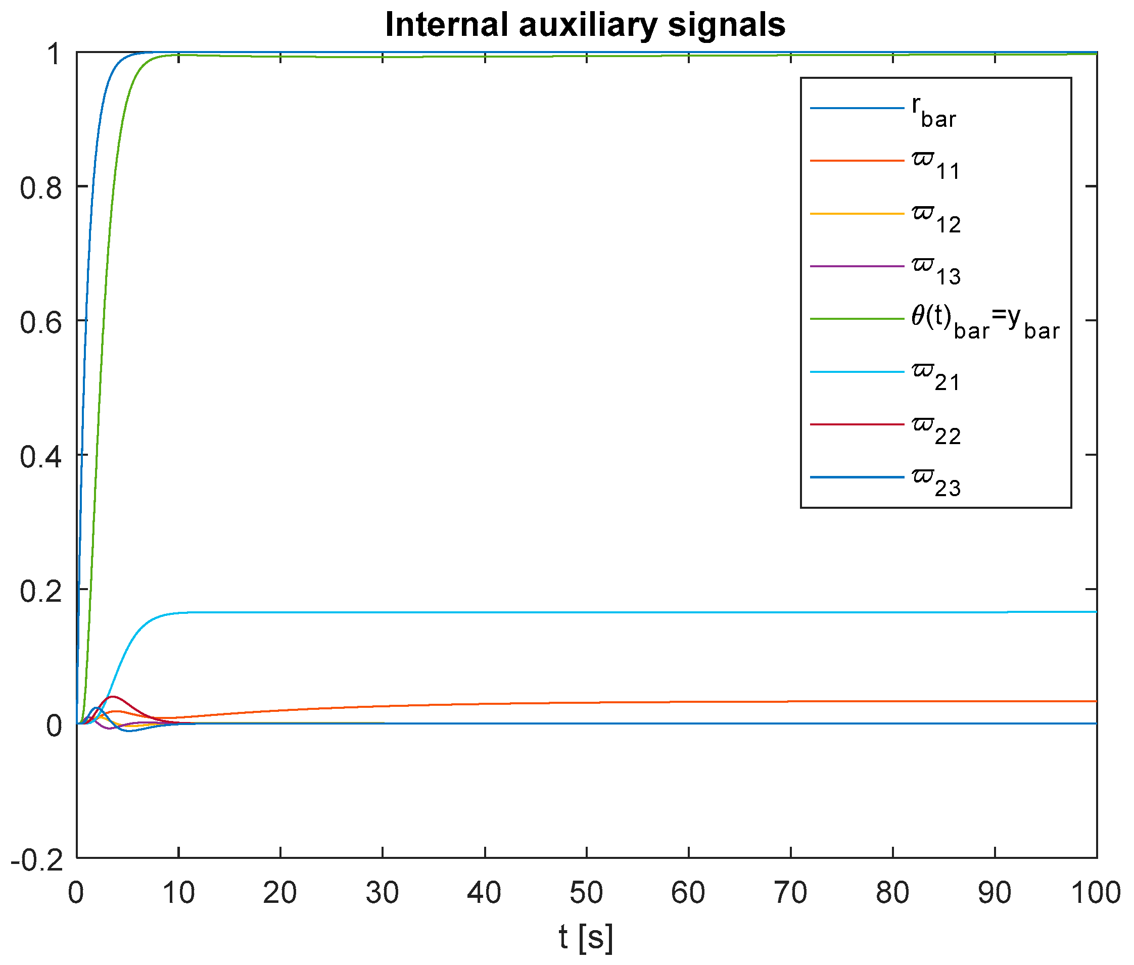
Finally, Figure 18 shows the boundedness of all auxiliary signals $\overline{\omega }$ of the FO-DMRAC when $n^{*}=2$. This is also true for the case when $n^{*}\ge 2$ is in the state of Lemma 3.

6. Conclusions

In this paper, we have analyzed and compared two types of adaptive controllers of the direct type that were applied to an integer order plant using integer and fractional order adjustment laws, namely, the classic or integer DMRAC (IO-DMRAC) and the FO-DMRAC. The simulation results allow us to verify the boundedness of all of the signals in the FO case, as assured by using Lemma 3. Moreover, through simulations, it was possible to show the advantages of the FO implementation, in particular when the relative degree of the plant is exactly equal to 2 ($n^{*}=2$). It was also possible to prove that the auxiliary signals $\omega \left(t\right)$ remain bounded without the need of using hypothesis (ii) of Theorem 1, thus relaxing the stability analysis.

It is promising to say that, when possible, it is useful to decrease the relative degree of the plant to 2, since the performance is better than in the cases of larger relative degrees, in which case one is obliged to use the generalized scheme ($n^{\mathrm{*}}\ge 2$) that is more complex to implement due to errors and auxiliary blocks. In addition, the fact that the output signal to be controlled is subject to oscillations and overshoots in the transient period, this phenomenon does not occur when case of $n^{\mathrm{*}}=2$ is considered. Finally, it is important to note, as said before, this is the first time that an FOAC is used in the longitudinal control of an airplane using fractional-order adaptive laws applied to an integer-order system (airplane model) without changing the classic structure of MRAC. Finally, the analysis of asymptotic stability is a subject still pending for future research work in the field of fractional-order MRAC control systems.

References

1. Seckel, E. Stability and Control of Airplane and Helicopters; Department of Aeronautical Engineering, The James Forrestal Research Center School of Engineering and Applied Science, Princeton University: Princeton, NJ, USA, 1964. [Google Scholar]
2. Roskam, J. Airplane Flight Dynamics and Automatic Flight Controls. Part 2; Roskam Aviation and Engineering Corporation: Lawrence, KS, USA, 1995. [Google Scholar]
3. Singh, B.; Urooj, S.; Singh, S. Analysis of autopilot system, integrated with modelling and comparison of different controllers with the system. J. Discret. Math. Sci. Cryptogr. 2020, 23, 1059–1068. [Google Scholar] [CrossRef]
4. Ponrani, M.A.; Godweena, A.K. Aircraft Pitch Control using PID Controller. In Proceedings of the International Conference on System, Computation, Automation and Networking (ICSCAN), Puducherry, India, 30–31 July 2021. [Google Scholar]
5. Alves, L.; Brito, V.; Palma, L.B.; Gil, B. Position Control in Simulated Airplanes. In Proceedings of the 2019 International Young Engineers Forum, Costa da Caparica, Portugal, 10 May 2019. [Google Scholar]
6. Blakelock, J. Automatic Control of Aircraft and Missiles; John Wiley & Sons, Inc.: New York, NY, USA, 1965. [Google Scholar]
7. Modi, V.J.; Mokhtarian, F.; Yokomizo, T. Effect of moving surface on the airfoil boundary-layer control. AIAA-J. Aircr. 1990, 27, 42–50. [Google Scholar] [CrossRef]
8. Duarte-Mermoud, M.A.; Rioseco, J.S.; González, R.I. Control of longitudinal movement of a plane using combined model reference adaptive control. Int. J. Aircr. Eng. Aerosp. Technol. 2005, 77, 199–213. [Google Scholar] [CrossRef]
9. Lavretsky, E. Combined/composite model reference adaptive control. IEEE Trans. Autom. Control. 2009, 54, 2692–2697. [Google Scholar] [CrossRef]
10. Mangiacasale, L. Airplane Control Systems: μ-Synthesis with MATLAB; Edizioni Levroto & Bella: Torino, Italy, 1996. [Google Scholar]
11. Al-Hiddabi, S.A.; McClamroch, N.H. Tracking and maneuver regulation control for nonlinear nonminimum phase system: Applications to flight control. IEEE Trans. Control Syst. Technol. 2002, 10, 780–792. [Google Scholar] [CrossRef]
12. Liang, Y.; Chen, X.; Xu, R. Research on Longitudinal Landing Track Control Technology of Carrier-based Aircraft. In Proceedings of the Chinese Control and Decision Conference (CCDC 2020), Hefei, China, 22–24 August 2020. [Google Scholar]
13. Yuxing, Z.; Jie, X.; Zhikuo, C. LQR Controller for Longitudinal Control Augmentation System of Aircraft Based on Hybrid Genetic Algorithm. In Proceedings of the IEEE CSAA Guidance, Navigation and Control Conference (CGNCC), Xiamen, China, 10–12 August 2018. [Google Scholar]
14. Lavretsky, E. Adaptive Output Feedback Design Using Asymptotic Properties of LQG/LTR Controllers. IEEE Trans. Autom. Control 2012, 57, 1587–1591. [Google Scholar] [CrossRef]
15. Doyle, J.C.; Stein, G. Multivariable feedback design: Concepts for a classical/modern synthesis. IEEE Trans. Autom. Control 1981, 26, 4–16. [Google Scholar] [CrossRef]
16. Safonov, M.; Laub, A.; Hartmann, G. Feedback properties of multivariable systems: The role and use of the return difference matrix. IEEE Trans. Autom. Control 1981, 26, 47–65. [Google Scholar] [CrossRef]
17. Stein, G.; Athans, M. The LQG/LTR procedure for multivariable feedback control design. IEEE Trans. Autom. Control 1987, 32, 105–114. [Google Scholar] [CrossRef]
18. Rimon, E.; Narendra, K. A new adaptive estimator for linear systems. IEEE Trans. Autom. Control 1992, 37, 410–412. [Google Scholar] [CrossRef]
19. Kreisselmeier, G. Adaptive Observers with Exponential Rate of Convergence. IEEE Trans. Autom. Control 1977, 22, 2–8. [Google Scholar] [CrossRef]
20. Rosario-Gabriel, I.; Cortes, H.R. Aircraft Longitudinal Control based on the Lanchester’s Phugoid Dynamics Model. In Proceedings of the International Conference on Unmanned Aircraft Systems (ICUAS), Dallas, TX, USA, 12–15 June 2018. [Google Scholar]
21. Sheng, S.; Sun, C.; Duan, H.; Jiang, X.; Zhu, Y.; Shouzhao, S.; Chenwu, S.; Haibin, D.; Xiaoliang, J.; Yansong, Z. Longitudinal and Lateral Adaptive Flight Control Design for an Unmanned Helicopter with Coaxial Rotor and Ducted Fan. In Proceedings of the 33rd Chinese Control Conference, Nanjing, China, 28–30 July 2014. [Google Scholar]
22. Ynineb, A.R.; Ladaci, S. MRAC Adaptive Control Design for an F15 Aircraft Pitch Angular Motion Using Dynamics Inversion and Fractional-Order Filtering. Int. J. Robot. Control Syst. 2022, 2, 240–252, ISSN 2775-2658. [Google Scholar] [CrossRef]
23. Johnson, B.J. High Angle of Attack Flight Characteristics of a Small UAV with a Variable-Size Vertical Tail. Ph. D. Thesis, University of Florida, Gainesville, FL, USA, 2009. [Google Scholar]
24. FAR 23, “Airworthiness Standards: Normal, Utility, Acrobatic and Commuter Category Airplanes”, Part 23, Chapter I, Federal Aviation Regulations, Title 14 Code of Federal Regulations (CFR), 1991. Available online: http://www.faa.gov (accessed on 10 February 2023).
25. Narendra, K.S.; Annaswamy, A.M. Stable Adaptive Systems; Dover Publications Inc.: Mineola, NY, USA, 2005. [Google Scholar]
26. Narendra, K.S.; Valavani, L.S. Stable Adaptive Controller Design-Direct Control. IEEE Trans. Autom. Control 1978, 23, 570–583. [Google Scholar] [CrossRef]
27. Kilbas, A.A.; Srivastava, H.M.; Trujillo, J.J. Theory and Applications of Fractional Differential Equations; Elsevier: Amsterdam, The Netherlands, 2006. [Google Scholar]
28. Diethelem, K. The Analysis of Fractional Differential Equations; Springer: Berlin/Heidelberg, Germany, 2010. [Google Scholar]
29. Duarte-Mermoud, M.A.; Aguila-Camacho, N.; Gallegos, J.A.; Castro-Linares, R. Using General Quadratic Lyapunov Functions to Prove Lyapunov Uniform Stability for Fractional Order Systems. Commun. Nonlinear Sci. Numer. Simul. 2015, 22, 650–659. [Google Scholar] [CrossRef]
30. Aguila-Camacho, N.; Duarte-Mermoud, M.A.; Gallegos, J.A. Lyapunov Functions for Fractional Order Systems. Commun. Nonlinear Sci. Numer. Simul. 2014, 19, 2951–2957. [Google Scholar] [CrossRef]
31. Aguila-Camacho, N.; Duarte-Mermoud, M.A. Boundedness of the solutions for certain classes of fractional differential equations with application to adaptive systems. ISA Trans. 2016, 60, 82–88. [Google Scholar] [CrossRef]
32. NAguila-Camacho, N.; Gallegos, J.; Duarte-Mermoud, M.A. Analysis of fractional order error models in adaptive systems: Mixed order cases. Fract. Calc. Appl. Anal. 2019, 22, 1113–1132. [Google Scholar] [CrossRef]
33. The Math Works Inc. Control System Toolbox User’s Guide. 1998. Available online: http://www.mathworks.com (accessed on 8 March 2022).
34. Rauw, M.O. FDC 1.2-A Simulating Toolbox for Flight Dynamics and Control Analysis; The Math Works Inc.: Natick, MA, USA, 1998. [Google Scholar]
35. Valerio, D.; Da Costa, J.S. Ninteger: A non-integer control toolbox for matlab. In Fractional Derivatives and Applications; OIFAC: Bordeaux, France, 2004. [Google Scholar]
36. Sabatier, J.; Aoun, M.; Oustaloup, A.; Gregoire, G.; Ragot, F.; Roy, P. Fractional system identification for lead acid battery state of charge estimation. Signal Process. 2006, 86, 2645–2657. [Google Scholar] [CrossRef]
37. Clerc, M. Particle Swarm Optimization; ISTE Ltd.: Hollywood, FL, USA, 2006. [Google Scholar]
Figure 2. Block diagram of the DMRAC scheme.
Fractalfract 07 00342 g002
Figure 3. Detailed block diagram of the DMRAC applied to the plane.
Fractalfract 07 00342 g003
Figure 4. Plant open−loop response under a unit step input.
Fractalfract 07 00342 g004
Figure 5. Structure of the DMRAC when the relative degree of the plant is n * = 1 .
Fractalfract 07 00342 g005
Figure 6. Block diagram associated to the output error e 1 ( t ) valid only for the case of an nth order plant with a relative degree exactly equal to 2.
Fractalfract 07 00342 g006
Figure 7. Simplified block diagram of the output error in the case of DMRAC for a plant of a relative degree n * = 2 .
Fractalfract 07 00342 g007
Figure 8. Open−loop system response to a unit step reference change at t = 0.
Fractalfract 07 00342 g008
Figure 9. Evolution of the objective function J n o r m as the number of iterations increases using PSO for the IO-DMRAC.
Fractalfract 07 00342 g009
Figure 10. Evolution of the objective function or cost function J n o r m as the number of iterations increases using PSO and FO-DMRAC.
Fractalfract 07 00342 g010
Figure 11. Pitch angle response θ t under IO-DMRAC and FO-DMRAC.
Fractalfract 07 00342 g011
Figure 12. Zoom of the variations of the pitch angle θ t shown in Figure 11 by using IO-DMRAC and FO-DMRAC.
Fractalfract 07 00342 g012
Figure 13. Control effort δ e t with FO-DMRAC and IO-DMRAC.
Fractalfract 07 00342 g013
Figure 14. Zoom of the control effort δ e t with FO-DMRAC and IO-DMRAC.
Fractalfract 07 00342 g014
Figure 15. General structure of the DMRAC for the case when the relative degree of the plant is n * 2 .
Fractalfract 07 00342 g015
Figure 16. Evolution of the pitch angle θ(t) with the generalized IO-DMRAC (black color) and FO-DMRAC (red color). The reference is shown in green (unit step).
Fractalfract 07 00342 g016
Figure 17. Zoom of the transient evolution of the control effort δ e t during the 10 first seconds. Black signal corresponds to the generalized IO-DMRAC structure case, and IO-DMRAC (blue color) and FO-DMRAC (red color) are the cases when the simple structure is used ( n * = 2 ).
Fractalfract 07 00342 g017
Figure 18. Auxiliary signals ω ¯ (all bounded).
Fractalfract 07 00342 g018