Application of the Pathway-Type Transform to a New Form of a Fractional Kinetic Equation Involving the Generalized Incomplete Wright Hypergeometric Functions

Abstract

We present in this paper a generalization of the fractional kinetic equation using the generalized incomplete Wright hypergeometric function. The pathway-type transform technique is then used to investigate the solutions to a fractional kinetic equation with specific fractional transforms. Furthermore, exceptional cases of our outcomes are discussed and graphically illustrated using MATLAB software. This work provides a thorough overview for further investigation into these topics in order to gain a better understanding of their implications and applications.

1. Introduction

Fractional-order differential equations have fractional derivatives instead of integer derivatives [1,2,3,4,5]. A kinetic equation is one of the essential kinds of fractional-order differential equations. Its importance is reflected in the fact that it has received increased attention in electrodynamics, control systems, economics, hydrodynamics, physics, geophysics, and mathematics. Furthermore, fractional-order kinetic (reaction-type) equations play a significant role as tools of mathematics that are frequently employed to describe a variety of physical and astrophysical phenomena (see [6,7,8,9,10]). For example, reaction-type (kinetic) equations can explain how nuclei are created and destroyed during chemical (thermonuclear) processes. A formal representation of reactions characterized by a time-dependent quantity $\mathbf{E}=\mathbf{E}\left(\xi \right)$ is given by the following Cauchy problem (see, for example, [11]):

$$\begin{array}{c}\hfill \frac{d\mathbf{E}}{d\xi }=-\delta \left(\mathbf{E}\right)+p\left(\mathbf{E}\right),\mathbf{E}\left(0\right)={\mathbf{E}}_0,\end{array}$$

(1)

where ${\mathbf{E}}_0$ is the initial data and $\delta$ and p are the destruction and production rate of $\mathbf{E}$, respectively. Furthermore, Haubold and Mathai studied a special case of this Cauchy problem [11] given by

$$\begin{array}{c}\hfill \frac{d\mathbf{E}}{d\xi }=-\vartheta \mathbf{E},\vartheta \in {\mathbb{R}}^{+},\mathbf{E}\left(0\right)={\mathbf{E}}_0.\end{array}$$

(2)

Equation (2) is known as the standard kinetic equation. They also gave a representation in the form of a fractional equation as follows:

$$\begin{array}{c}\hfill \mathbf{E}\left(\xi \right)-{\mathbf{E}}_0=-\vartheta {}_0{\mathbb{D}}_{\xi }^{-1}\mathbf{E}\left(\xi \right),\vartheta ,\xi \in {\mathbb{R}}^{+},\end{array}$$

(3)

where ${}_0{\mathbb{D}}_{\xi }^{-\nu }$ is the fractional integral operator [1] given by

$$\begin{array}{c}\hfill {}_0{\mathbb{D}}_{\xi }^{-\nu }f\left(\xi \right)=\frac{1}{\Gamma \left(\nu \right)}{\int }_0^{\xi }{(\xi -s)}^{\nu -1}f\left(s\right)ds,\nu \in {\mathbb{R}}^{+}.\end{array}$$

(4)

Many generalizations and solutions of the fractional-order kinetic equation have recently been developed, utilizing a variety of fractional integral transforms including the fractional Laplace transform [12,13,14,15,16], fractional Sumudu transform [17,18,19], Hadamard fractional integrals [20,21,22], fractional pathway transform [23,24] and Prabhakar-type operators [25], which have been extensively studied. In particular, Khan et al. [14] presented solutions for fractional kinetic equations associated with the $(p,q)$-extended $\tau$-hypergeometric and confluent hypergeometric functions using the Laplace transform, while Hidan et al. [15] discussed a technique for the Laplace transformation of solutions of fractional kinetic equations involving extended $(k,t)$-Gauss hypergeometric matrix functions. In addition, Abubakar [16] derived solutions for fractional kinetic equations using the $(p,q;l)$-extended $\tau$-Gauss hypergeometric function. Gaining insight from the last recently mentioned manuscripts, this paper provides an in-depth exploration of fractional kinetic equations and their solutions by using the generalized incomplete Wright hypergeometric function and pathway-type transform technique. We provide a comprehensive overview that is sure to give researchers plenty to think about when it comes to implications and applications. Overall, this work should be regarded as required reading for anyone interested in learning more about these themes.

2. Preliminaries

Here, we highlight a few concepts that would be helpful for future discussion.

The Gauss hypergeometric function given by

$$\begin{array}{c}\hfill \mathbf{F}({\theta }_1,{\theta }_2,{\theta }_3;z)=\sum _{j=0}^{\infty }\frac{{\left({\theta }_1\right)}_j{\left({\theta }_2\right)}_j}{{\left({\theta }_3\right)}_j}\frac{z^j}{j!},z\in \mathbb{C},\end{array}$$

(5)

will be convergent absolutely and uniformly under the condition $\left|z\right|<1$. Here, ${\theta }_1,{\theta }_2$, and ${\theta }_3$ are complex parameters with ${\theta }_3\in \mathbb{C}\backslash {\mathbb{Z}}_0^{-}$, and

$$\begin{array}{c}\hfill {\left({\theta }_1\right)}_j=\frac{\Gamma ({\theta }_1+j)}{\Gamma \left({\theta }_1\right)}=\left\{\begin{array}{cc}{\theta }_1({\theta }_1+1)\cdots ({\theta }_1+j-1),\hfill & j\in \mathbb{N},{\theta }_1\in \mathbb{C}\hfill \\ \\ 1,\hfill & j=0;{\theta }_1\in \mathbb{C}\backslash \left\{0\right\},\hfill \end{array}\right.\end{array}$$

(6)

is known to be the Pochhammer symbol of ${\theta }_1$, whereas $\Gamma \left(v\right)$ is the standard gamma function, defined as

$$\begin{array}{c}\hfill \Gamma \left(\theta \right)={\int }_0^{\infty }{\upsilon }^{\theta -1}{e}^{-\upsilon }d\upsilon ,\theta \in \mathbb{C}\backslash {\mathbb{Z}}_0^{-}.\end{array}$$

(7)

Moreover, we define the lower and upper incomplete gamma functions, as shown in [26], as

$$\begin{array}{c}\hfill \gamma (\theta ;x)={\int }_0^x{\upsilon }^{\theta -1}{e}^{-\upsilon }d\upsilon ,\theta \in \mathbb{C}\backslash {\mathbb{Z}}_0^{-},\end{array}$$

(8)

and

$$\begin{array}{c}\hfill \Gamma (\theta ;x)={\int }_x^{\infty }{\upsilon }^{\theta -1}{e}^{-\upsilon }d\upsilon ,\theta \in \mathbb{C}\backslash {\mathbb{Z}}_0^{-},\end{array}$$

(9)

respectively. The decomposition formula of $\Gamma \left(\theta \right)$ can be preformed using Equations (8) and (9) as follows:

$$\begin{array}{c}\hfill \gamma (\theta ;x)+\Gamma (\theta ;x)=\Gamma \left(\theta \right).\end{array}$$

(10)

The incomplete Pochhammer symbols ${(\theta ;x)}_n$ and ${[\theta ;x]}_n$ are defined by

$$\begin{array}{c}\hfill {(\theta ;x)}_n=\frac{\gamma (\theta +n;x)}{\Gamma \left(\theta \right)}\end{array}$$

(11)

and

$$\begin{array}{c}\hfill {[\theta ;x]}_n=\frac{\Gamma (\theta +n;x)}{\Gamma \left(\theta \right)}.\end{array}$$

(12)

Similar to Equation (10), a decomposition of ${\left(\theta \right)}_n$ can be given by the functions in Equations (11) and (12) as follows:

$$\begin{array}{c}\hfill {(\theta ;x)}_n+{[\theta ;x]}_n={\left(\theta \right)}_n,\end{array}$$

(13)

Wright’s $(\tau -Gauss)$ hypergeometric function was first studied in [27] as follows:

$$\begin{array}{c}\hfill \begin{array}{c}\hfill {}_2{\mathbf{R}}_1^{}({\vartheta }_1,{\vartheta }_2;{\vartheta }_3;\tau ;\eta )=\frac{\Gamma \left({\vartheta }_3\right)}{\Gamma \left({\vartheta }_2\right)}\sum _{j=0}^{\infty }\frac{{\left({\vartheta }_1\right)}_j\Gamma ({\vartheta }_2+\tau j)}{\Gamma ({\vartheta }_3+\tau j)}\frac{{\eta }^j}{j!}(\tau \in {\mathbb{R}}^{+},\left|\eta \right|<1),\end{array}\end{array}$$

(14)

where ${\vartheta }_1,{\vartheta }_2$, and ${\vartheta }_3$ are complex parameters such that $\Re \left({\vartheta }_1\right)>0,\Re \left({\vartheta }_2\right)>0$, and $\Re \left({\vartheta }_3\right)>0$.

In addition, the incomplete Wright’s hypergeometric function was studied in [28] as follows:

$$\begin{array}{c}\hfill \begin{array}{c}\hfill {}_2{\Gamma }_1^{}({\vartheta }_1,{\vartheta }_2;{\vartheta }_3;\tau ;\eta )=\frac{\Gamma \left({\vartheta }_3\right)}{\Gamma \left({\vartheta }_2\right)}\sum _{j=0}^{\infty }\frac{{[{\vartheta }_1;x]}_j\Gamma ({\vartheta }_2+\tau j)}{\Gamma ({\vartheta }_3+\tau j)}\frac{{\eta }^j}{j!}(\tau \in {\mathbb{R}}^{+},\left|\eta \right|<1)\end{array}\end{array}$$

(15)

and

$$\begin{array}{c}\hfill \begin{array}{c}\hfill {}_2{\gamma }_1^{}({\vartheta }_1,{\vartheta }_2;{\vartheta }_3;\tau ;\eta )=\frac{\Gamma \left({\vartheta }_3\right)}{\Gamma \left({\vartheta }_2\right)}\sum _{j=0}^{\infty }\frac{{({\vartheta }_1;x)}_j\Gamma ({\vartheta }_2+\tau j)}{\Gamma ({\vartheta }_3+\tau j)}\frac{{\eta }^j}{j!}(\tau \in {\mathbb{R}}^{+},\left|\eta \right|<1),\end{array}\end{array}$$

(16)

where ${\vartheta }_1,{\vartheta }_2$, and ${\vartheta }_3$ are complex parameters such that $\Re \left({\vartheta }_1\right)>0,\Re \left({\vartheta }_2\right)>0$, and $\Re \left({\vartheta }_3\right)>0.$ Recent developments and expansions of Wright’s hypergeometric function can be found, for example, in [29,30].

The family of the generalized incomplete Wright’s hypergeometric functions of the p numerator and q denominator is given by [28]

$$\begin{array}{c}\hfill \begin{array}{cc}\hfill {}_p{\Gamma }_q^{\left(\tau \right)}\left[\begin{array}{c}({\theta }_p,x);\\ {\eta }_q;\end{array}z\right]& ={}_p{\Gamma }_q^{\left(\tau \right)}\left[\begin{array}{c}({\theta }_1,x),{\theta }_2,\dots ,{\theta }_p;\\ {\eta }_1,{\eta }_2,\dots ,{\eta }_q;\end{array}z\right]\hfill \\ & =\frac{\Gamma \left({\eta }_1\right),\dots ,\Gamma \left({\eta }_q\right)}{\Gamma \left({\theta }_2\right),\dots ,\Gamma \left({\theta }_p\right)}\sum _{n=0}^{\infty }\frac{{[{\theta }_1,x]}_n\Gamma ({\theta }_2+n\tau )\dots \Gamma ({\theta }_p+n\tau )}{\Gamma ({\eta }_1+n\tau )\Gamma ({\eta }_2+n\tau )\dots \Gamma ({\eta }_q+n\tau )}\frac{z^n}{n!},\hfill \end{array}\end{array}$$

(17)

where ${\vartheta }_p,{\eta }_q\in \mathbb{C},\tau >0,p=q+1,p,q\in {\mathbb{N}}_0,\left|z\right|<1$, and

$$\begin{array}{c}\hfill \begin{array}{cc}\hfill {}_p{\gamma }_q^{\left(\tau \right)}\left[\begin{array}{c}({\theta }_p,x);\\ {\eta }_q;\end{array}z\right]& ={}_p{\gamma }_q^{\left(\tau \right)}\left[\begin{array}{c}({\theta }_1,x),{\theta }_2,\dots ,{\theta }_p;\\ {\eta }_1,{\eta }_2,\dots ,{\eta }_q;\end{array}z\right]\hfill \\ & =\frac{\Gamma \left({\eta }_1\right),\dots ,\Gamma \left({\eta }_q\right)}{\Gamma \left({\theta }_2\right),\dots ,\Gamma \left({\theta }_p\right)}\sum _{n=0}^{\infty }\frac{{({\theta }_1,x)}_n\Gamma ({\theta }_2+n\tau )\dots \Gamma ({\theta }_p+n\tau )}{\Gamma ({\eta }_1+n\tau )\Gamma ({\eta }_2+n\tau )\dots \Gamma ({\eta }_q+n\tau )}\frac{z^n}{n!},\hfill \end{array}\end{array}$$

(18)

where ${\vartheta }_p,{\eta }_q\in \mathbb{C},\tau >0,p=q+1$, and $p,q\in {\mathbb{N}}_0,\left|z\right|<1$.

The generalized incomplete hypergeometric functions ${}_p{\Gamma }_q^{\left(\tau \right)}$ and ${}_p{\gamma }_q^{\left(\tau \right)}$ satisfy the following decomposition formula:

$$\begin{array}{c}\hfill \begin{array}{c}\hfill {}_p{\Gamma }_q^{\left(\tau \right)}\left[\begin{array}{c}({\theta }_p,x);\\ {\eta }_q;\end{array}z\right]+{}_p{\gamma }_q^{\left(\tau \right)}\left[\begin{array}{c}({\theta }_p,x);\\ {\eta }_q;\end{array}z\right]{=}_p{\mathbf{R}}_q^{\left(\tau \right)}\left[\begin{array}{c}{\theta }_p;\\ {\eta }_q;\end{array}z\right]\end{array}\end{array}$$

(19)

Remark 1. 

Some special cases of the generalized incomplete Wright’s hypergeometric functions are as follows:

(i) 

By setting $\tau =1$ in Equations (17) and (18) and employing the relation in Equation (6), we have the extended incomplete Gauss hypergeometric function (see [31]):

$$\begin{array}{c}\hfill \begin{array}{cc}\hfill {}_p{\Gamma }_q\left[\begin{array}{c}({\theta }_p,x);\\ {\eta }_q;\end{array}z\right]& ={}_p{\Gamma }_q\left[\begin{array}{c}({\theta }_1,x),{\theta }_2,\dots ,{\theta }_p;\\ {\eta }_1,{\eta }_2,\dots ,{\eta }_q;\end{array}z\right]\hfill \\ & =\sum _{n=0}^{\infty }\frac{{[{\theta }_1,x]}_n{\left({\theta }_2\right)}_n+\dots {\left({\theta }_p\right)}_n}{{\left({\eta }_1\right)}_n\dots {\left({\eta }_q\right)}_n}\frac{z^n}{n!},\hfill \end{array}\end{array}$$

(20)

where ${\vartheta }_p,{\eta }_q\in \mathbb{C},\tau >0,p=q+1,p,q\in {\mathbb{N}}_0,\left|z\right|<1$, and

$$\begin{array}{c}\hfill \begin{array}{cc}\hfill {}_p{\gamma }_q\left[\begin{array}{c}({\theta }_p,x);\\ {\eta }_q;\end{array}z\right]& ={}_p{\gamma }_q\left[\begin{array}{c}({\theta }_1,x),{\theta }_2,\dots ,{\theta }_p;\\ {\eta }_1,{\eta }_2,\dots ,{\eta }_q;\end{array}z\right]\hfill \\ & =\sum _{n=0}^{\infty }\frac{{({\theta }_1,x)}_n{\left({\theta }_2\right)}_n+\dots {\left({\theta }_p\right)}_n}{{\left({\eta }_1\right)}_n\dots {\left({\eta }_q\right)}_n}\frac{z^n}{n!},\hfill \end{array}\end{array}$$

(21)

where ${\vartheta }_p,{\eta }_q\in \mathbb{C},\tau >0,p=q+1$, and $p,q\in {\mathbb{N}}_0,\left|z\right|<1$.

As an immediate consequence of Equations (20) and (21), we have the following decomposition formula:

$$\begin{array}{c}\hfill \begin{array}{c}\hfill {}_p{\Gamma }_q\left[\begin{array}{c}({\theta }_p,x);\\ {\eta }_q;\end{array}z\right]+{}_p{\gamma }_q\left[\begin{array}{c}({\theta }_p,x);\\ {\eta }_q;\end{array}z\right]{=}_p{\mathbf{F}}_q\left[\begin{array}{c}{\theta }_p;\\ {\eta }_q;\end{array}z\right],\end{array}\end{array}$$

(22)

in terms of the generalized hypergeometric function.

(ii) 

If we put $p=2$ and $q=1$ into Equations (17) and (18), we obtain

$$\begin{array}{c}\hfill \begin{array}{cc}\hfill {}_2{\Gamma }_1^{\left(\tau \right)}\left[\begin{array}{c}({\theta }_2,x);\\ {\eta }_1;\end{array}z\right]& ={}_p{\Gamma }_q^{\left(\tau \right)}\left[\begin{array}{c}({\theta }_1,x),{\theta }_2;\\ {\eta }_1;\end{array}z\right]\hfill \\ & =\frac{\Gamma \left({\eta }_1\right)}{\Gamma \left({\theta }_2\right)}\sum _{n=0}^{\infty }\frac{{[{\theta }_1,x]}_n\Gamma ({\theta }_2+n\tau )}{\Gamma ({\eta }_1+n\tau )\Gamma ({\eta }_2+n\tau )}\frac{z^n}{n!},\hfill \\ & (\tau >0,|z|<1),\hfill \end{array}\end{array}$$

(23)

and

$$\begin{array}{c}\hfill \begin{array}{cc}\hfill {}_2{\gamma }_1^{\left(\tau \right)}\left[\begin{array}{c}({\theta }_2,x);\\ {\eta }_1;\end{array}z\right]& ={}_2{\gamma }_1^{\left(\tau \right)}\left[\begin{array}{c}({\theta }_1,x),{\theta }_2;\\ {\eta }_1;\end{array}z\right]\hfill \\ & =\frac{\Gamma \left({\eta }_1\right))}{\Gamma \left({\theta }_2\right)}\sum _{n=0}^{\infty }\frac{{({\theta }_1,x)}_n\Gamma ({\theta }_2+n\tau )}{\Gamma ({\eta }_1+n\tau )}\frac{z^n}{n!},\hfill \\ & (\tau >0,|z|<1).\hfill \end{array}\end{array}$$

(24)

Equations (23) and (24) contain the following decomposition formula as a direct result:

$$\begin{array}{c}\hfill \begin{array}{c}\hfill {}_2{\Gamma }_1^{\left(\tau \right)}\left[\begin{array}{c}({\theta }_1,x),{\theta }_2;\\ {\eta }_1;\end{array}z\right]+{}_2{\gamma }_1^{\left(\tau \right)}\left[\begin{array}{c}({\theta }_1,x),{\theta }_2;\\ {\eta }_1;\end{array}z\right]{=}_2{\mathbf{R}}_1^{\left(\tau \right)}\left[\begin{array}{c}{\theta }_1,{\theta }_2;\\ {\eta }_1;\end{array}z\right]\end{array}\end{array}$$

(25)

for the Wright hypergeometric function in (14).

The derivative formulas for generalized incomplete Wright’s hypergeometric functions are as follows (see [28]):

$$\begin{array}{c}\hfill \begin{array}{cc}\hfill & \frac{{\mathrm{d}}^n}{\mathrm{d}{z}^n}\left\{{}_p{\Gamma }_q^{\left(\tau \right)}\left[\begin{array}{c}({\theta }_1,x),{\theta }_2,\dots ,{\theta }_p;\\ {\eta }_1,{\eta }_2,\dots ,{\eta }_q;\end{array}z\right]\right\}\hfill \\ & =\frac{{\left({\theta }_1\right)}_n\Gamma ({\theta }_2+n\tau )\dots \Gamma ({\theta }_p+n\tau )}{\Gamma ({\eta }_1+n\tau )\Gamma ({\eta }_2+n\tau )\dots \Gamma ({\eta }_q+n\tau )}\hfill \\ & \times {}_p{\Gamma }_q^{\left(\tau \right)}\left[\begin{array}{c}({\theta }_1+n,x),{\theta }_2+n\tau ,\dots ,{\theta }_p+n\tau ;\\ {\eta }_1+n\tau ,{\eta }_2+n\tau ,\dots ,{\eta }_q+n\tau ;\end{array}z\right]\hfill \end{array}\end{array}$$

(26)

and

$$\begin{array}{c}\hfill \begin{array}{cc}\hfill & \frac{{\mathrm{d}}^n}{\mathrm{d}{z}^n}\left\{{}_p{\gamma }_q^{\left(\tau \right)}\left[\begin{array}{c}({\theta }_1,x),{\theta }_2,\dots ,{\theta }_p;\\ {\eta }_1,{\eta }_2,\dots ,{\eta }_q;\end{array}z\right]\right\}\hfill \\ & =\frac{{\left({\theta }_1\right)}_n\Gamma ({\theta }_2+n\tau )\dots \Gamma ({\theta }_p+n\tau )}{\Gamma ({\eta }_1+n\tau )\Gamma ({\eta }_2+n\tau )\dots \Gamma ({\eta }_q+n\tau )}\hfill \\ & {\times }_p{\gamma }_q^{\left(\tau \right)}\left[\begin{array}{c}({\theta }_1+n,x),{\theta }_2+n\tau ,\dots ,{\theta }_p+n\tau ;\\ {\eta }_1+n\tau ,{\eta }_2+n\tau ,\dots ,{\eta }_q+n\tau ;\end{array}z\right].\hfill \end{array}\end{array}$$

(27)

The pathway-type transform (${\mathbf{K}}_{\omega }$ transform) is defined in [23,24] as

$$\begin{array}{c}\hfill {\mathbf{K}}_{\omega }[f\left(t\right),s]=F\left(s\right)={\int }_0^{\infty }{[1+(\omega -1)s]}^{\frac{-t}{\omega -1}}f\left(t\right)dt\omega >1,\end{array}$$

(28)

with

$$\begin{array}{c}\hfill \underset{\omega \to 1^{+}}{lim}{[1+(\omega -1)s]}^{\frac{-t}{\omega -1}}=e^{-st}.\end{array}$$

(29)

The Laplace transform $\left(L\right[.,.\left]\right)$ is generalized by this transformation; which can be seen from

$$\begin{array}{c}\hfill \underset{\omega \to 1}{lim}{\mathbf{K}}_{\omega }[f\left(t\right),s]=L[f\left(t\right),s].\end{array}$$

(30)

The two useful properties of the ${\mathbf{K}}_{\omega }$ transform are as follows:

$$\begin{array}{c}\hfill {\mathbf{K}}_{\omega }[1,s]=\frac{\omega -1}{\ln [1+(\omega -1\left)s\right]}\end{array}$$

(31)

and

$$\begin{array}{c}\hfill {\mathbf{K}}_{\omega }[\frac{t^n}{n!},s]={\left\{\frac{\omega }{\ln [1+(\omega -1\left)s\right]}\right\}}^{n+1}.\end{array}$$

(32)

Furthermore, using the convolution theorem of the ${\mathbf{K}}_{\omega }$ transform [23], we see that Equation (4) may be represented by

$$\begin{array}{c}\hfill {\mathbf{K}}_{\omega }{[}_0{\mathbb{D}}_t^{-\lambda }f\left(t\right),s]={\left[\frac{\omega -1}{\ln [1+(\omega -1\left)s\right]}\right]}^{\lambda }{\mathbf{K}}_{\omega }[f\left(t\right),s]\lambda \in \mathbb{C}.\end{array}$$

(33)

3. Statement of Results

In this section, we solve the fractional kinetic equation associated with the $\tau$-generalized incomplete hypergeometric functions using the method of the ${\mathbf{K}}_{\omega }$ transform.

Theorem 1. 

Let $\lambda >0,d>0,z\in \mathbb{C}$, and $\tau >0$. Then, we conclude that the solution of the τ-generalized incomplete hypergeometric function’s fractional kinetic equation

$$\begin{array}{c}\hfill \mathbf{E}\left(z\right)-{\mathbf{E}}_0{}_p{\Gamma }_q^{\left(\tau \right)}\left(z\right)=-d^{\lambda }{}_0{\mathbb{D}}_z^{-\lambda }\mathbf{E}\left(z\right),\end{array}$$

(34)

is given by

$$\begin{array}{c}\hfill \begin{array}{cc}\hfill \mathbf{E}\left(z\right)=& {\mathbf{E}}_0\frac{\Gamma \left({\eta }_1\right),\dots ,\Gamma \left({\eta }_q\right)}{\Gamma \left({\theta }_2\right),\dots ,\Gamma \left({\theta }_p\right)}\sum _{n=0}^{\infty }\frac{{[{\theta }_1,x]}_n\Gamma ({\theta }_2+n\tau )\dots \Gamma ({\theta }_p+n\tau )}{\Gamma ({\eta }_1+n\tau )\Gamma ({\eta }_2+n\tau )\dots \Gamma ({\eta }_q+n\tau )}\hfill \\ \hfill \times & \sum _{m=0}^{\infty }{(-1)}^m{\left(d\right)}^{m\lambda }\frac{z^{m\lambda +n}}{(m\lambda +n)!}.\hfill \end{array}\end{array}$$

(35)

Proof. 

By using the ${\mathbf{K}}_{\omega }$ transform of both sides of Equation (34) and using Equations (32) and (33), we have

$$\begin{array}{c}\hfill \begin{array}{cc}& {\mathbf{K}}_{\omega }\left[\mathbf{E}\left(z\right)\right]\left[1+d^{\lambda }{\left\{\frac{\omega -1}{\ln \{1+(\omega -1\left)r\right\}}\right\}}^{\lambda }\right]\hfill \\ & ={\mathbf{E}}_0\frac{\Gamma \left({\eta }_1\right),\dots ,\Gamma \left({\eta }_q\right)}{\Gamma \left({\theta }_2\right),\dots ,\Gamma \left({\theta }_p\right)}\sum _{n=0}^{\infty }\frac{{[{\theta }_1,x]}_n\Gamma ({\theta }_2+n\tau )\dots \Gamma ({\theta }_p+n\tau )}{\Gamma ({\eta }_1+n\tau )\Gamma ({\eta }_2+n\tau )\dots \Gamma ({\eta }_q+n\tau )}\hfill \\ & \times {\left[\frac{\ln \{1+(\omega -1\left)\right\}}{\omega -1}\right]}^{-n-1}\hfill \end{array}\end{array}$$

(36)

and

$$\begin{array}{c}\hfill \begin{array}{cc}\hfill {\mathbf{K}}_{\omega }\left[\mathbf{E}\left(z\right)\right]=& {\mathbf{E}}_0\frac{\Gamma \left({\eta }_1\right),\dots ,\Gamma \left({\eta }_q\right)}{\Gamma \left({\theta }_2\right),\dots ,\Gamma \left({\theta }_p\right)}\sum _{n=0}^{\infty }\frac{{[{\theta }_1,x]}_n\Gamma ({\theta }_2+n\tau )\dots \Gamma ({\theta }_p+n\tau )}{\Gamma ({\eta }_1+n\tau )\Gamma ({\eta }_2+n\tau )\dots \Gamma ({\eta }_q+n\tau )}\hfill \\ & {\left[\frac{\ln \{1+(\omega -1\left)r\right\}}{\omega -1}\right]}^{-n-1}\sum _{m=0}^{\infty }\frac{{(-1)}^m}{m!}{\left[\frac{d(\omega -1)}{\ln \{1+(\omega -1\left)r\right\}}\right]}^{m\lambda }\hfill \\ & ={\mathbf{E}}_0\frac{\Gamma \left({\eta }_1\right),\dots ,\Gamma \left({\eta }_q\right)}{\Gamma \left({\theta }_2\right),\dots ,\Gamma \left({\theta }_p\right)}\sum _{n=0}^{\infty }\frac{{[{\theta }_1,x]}_n\Gamma ({\theta }_2+n\tau )\dots \Gamma ({\theta }_p+n\tau )}{\Gamma ({\eta }_1+n\tau )\Gamma ({\eta }_2+n\tau )\dots \Gamma ({\eta }_q+n\tau )}\hfill \\ & \times \sum _{m=0}^{\infty }{(-1)}^m{d}^{m\lambda }{(\omega -1)}^{n+m\lambda +1}{\left[\ln \{1+(\omega -1\left)r\right\}\right]}^{-(n+m\lambda +1)}.\hfill \end{array}\end{array}$$

(37)

Now, when we take the inverse of the ${\mathbf{K}}_{\omega }$ transform and apply Equation (32), we have the desired result. □

Theorem 2. 

Let $\lambda >0,d>0,z\in C$, and $\tau >0$. Then, we conclude that the solution of the τ-generalized incomplete hypergeometric function’s fractional kinetic equation

$$\begin{array}{c}\hfill \mathbf{E}\left(z\right)-{\mathbf{E}}_0\{\frac{\mathrm{d}}{\mathrm{d}z}{}_p{\Gamma }_q^{(\tau )}(z)\}=-d^{\lambda }{}_0{\mathbb{D}}_t^{-\lambda }\mathbf{E}\left(z\right),\end{array}$$

(38)

is given by

$$\begin{array}{c}\hfill \begin{array}{cc}\hfill \mathbf{E}\left(z\right)=& {\mathbf{E}}_0\left[\frac{{\theta }_1({\theta }_2+\tau )\dots ({\theta }_p+\tau )}{({\eta }_1+\tau )\dots ({\eta }_q+\tau )}\right]\sum _{n=0}^{\infty }\frac{{[{\theta }_1+1,x]}_n{({\theta }_2+\tau )}_n\dots {({\theta }_p+\tau )}_n}{{({\eta }_1+\tau )}_n{({\eta }_2+\tau )}_n\dots {({\eta }_q+\tau )}_n}{z}^n\hfill \\ \hfill \times & \sum _{m=0}^{\infty }\frac{{(-1)}^m{\left(dz\right)}^{m\lambda }}{(m\lambda +n)!}.\hfill \end{array}\end{array}$$

(39)

Proof. 

By taking the ${\mathbf{K}}_{\omega }$ transform of both sides of Equation (38) and using Equations (26), (32), and (33), we find

$$\begin{array}{c}\hfill \begin{array}{cc}& {\mathbf{K}}_{\omega }\left[\mathbf{E}\left(z\right)\right]\left[1+d^{\lambda }{\left\{\frac{\omega -1}{\ln \{1+(\omega -1\left)r\right\}}\right\}}^{\lambda }\right]\hfill \\ \hfill =& {\mathbf{E}}_0\left[\frac{{\theta }_1({\theta }_2+\tau )\dots ({\theta }_p+\tau )}{({\eta }_1+\tau )\dots ({\eta }_q+\tau )}\right]\sum _{n=0}^{\infty }\frac{{[{\theta }_1+1,x]}_n{({\theta }_2+\tau )}_n\dots {({\theta }_p+\tau )}_n}{{({\eta }_1+\tau )}_n{({\eta }_2+\tau )}_n\dots {({\eta }_q+\tau )}_n}\hfill \\ \hfill \times & {\left[\frac{\ln \{1+(\omega -1\left)r\right\}}{\omega -1}\right]}^{-n-1}\hfill \end{array}\end{array}$$

(40)

and

$$\begin{array}{c}\hfill \begin{array}{cc}\hfill {\mathbf{K}}_{\omega }\left[\mathbf{E}\left(z\right)\right]=& {\mathbf{E}}_0\left[\frac{{\theta }_1({\theta }_2+\tau )\dots ({\theta }_p+\tau )}{({\eta }_1+\tau )\dots ({\eta }_q+\tau )}\right]\sum _{n=0}^{\infty }\frac{{[{\theta }_1+1,x]}_n{({\theta }_2+\tau )}_n\dots {({\theta }_p+\tau )}_n}{{({\eta }_1+\tau )}_n{({\eta }_2+\tau )}_n\dots {({\eta }_q+\tau )}_n}\hfill \\ & {\left[\frac{\ln \{1+(\omega -1\left)r\right\}}{\omega -1}\right]}^{-n-1}\sum _{m=0}^{\infty }\frac{{(-1)}^m}{m!}{\left[\frac{d(\omega -1)}{\ln \{1+(\omega -1\left)r\right\}}\right]}^{m\lambda }\hfill \\ \hfill =& {\mathbf{E}}_0\left[\frac{{\theta }_1({\theta }_2+\tau )\dots ({\theta }_p+\tau )}{({\eta }_1+\tau )\dots ({\eta }_q+\tau )}\right]\sum _{n=0}^{\infty }\frac{{[{\theta }_1+1,x]}_n{({\theta }_2+\tau )}_n\dots {({\theta }_p+\tau )}_n}{{({\eta }_1+\tau )}_n{({\eta }_2+\tau )}_n\dots {({\eta }_q+\tau )}_n}\hfill \\ \hfill \times & \sum _{m=0}^{\infty }{(-1)}^m{d}^{m\lambda }{(\omega -1)}^{n+m\lambda +1}{\left[\ln \{1+(\omega -1\left)r\right\}\right]}^{-(n+m\lambda +1)}.\hfill \end{array}\end{array}$$

(41)

By taking the inverse of the ${\mathbf{K}}_{\omega }$ transform of both sides of Equation (41) and applying Equation (32), we readily obtain the desired result. □

Now, we give the results for the solution of the fractional kinetic equation of the ${}_p{\gamma }_q^{\left(\tau \right)}$-generalized incomplete hypergeometric function in Equation (27), which are given in the following two theorems:

Theorem 3. 

Let $\lambda >0,d>0,z\in \mathbb{C}$, and $\tau >0$. Then, the solution of the fractional kinetic equation of the τ-generalized incomplete hypergeometric functions

$$\mathbf{E}\left(z\right)-{\mathbf{E}}_0{}_p{\gamma }_q^{\left(\tau \right)}\left(z\right)=-d^{\lambda }{}_0{\mathbb{D}}_z^{-\lambda }\mathbf{E}\left(z\right),$$

(42)

is given by

$$\begin{array}{c}\hfill \begin{array}{cc}\hfill \mathbf{E}\left(z\right)=& {\mathbf{E}}_0\frac{\Gamma \left({\eta }_1\right),\dots ,\Gamma \left({\eta }_q\right)}{\Gamma \left({\theta }_2\right),\dots ,\Gamma \left({\theta }_p\right)}\sum _{n=0}^{\infty }\frac{{({\theta }_1,x)}_n\Gamma ({\theta }_2+n\tau )\dots \Gamma ({\theta }_p+n\tau )}{\Gamma ({\eta }_1+n\tau )\Gamma ({\eta }_2+n\tau )\dots \Gamma ({\eta }_q+n\tau )}\hfill \\ \hfill \times & \sum _{m=0}^{\infty }{(-1)}^m{\left(d\right)}^{m\lambda }\frac{z^{m\lambda +n}}{(m\lambda +n)!}.\hfill \end{array}\end{array}$$

(43)

Proof. 

The proof here runs in parallel with that for Theorem 1. The details have been omitted. □

Theorem 4. 

Let $\lambda >0,d>0,z\in \mathbb{C}$, and $\tau >0$. Then, the solution of the fractional kinetic equation of the τ-generalized incomplete hypergeometric functions

$$\mathbf{E}(z)-{\mathbf{E}}_0\{\frac{\mathrm{d}}{\mathrm{d}z}{}_p{\gamma }_q^{(\tau )}(z)\}=-d^{\lambda }{}_0{\mathbb{D}}_t^{-\lambda }\mathbf{E}(z),$$

(44)

is given by

$$\begin{array}{c}\hfill \begin{array}{cc}\hfill \mathbf{E}\left(z\right)=& {\mathbf{E}}_0\left[\frac{{\theta }_1({\theta }_2+\tau )\dots ({\theta }_p+\tau )}{({\eta }_1+\tau )\dots ({\eta }_q+\tau )}\right]\sum _{n=0}^{\infty }\frac{{({\theta }_1+1,x)}_n{({\theta }_2+\tau )}_n\dots {({\theta }_p+\tau )}_n}{{({\eta }_1+\tau )}_n{({\eta }_2+\tau )}_n\dots {({\eta }_q+\tau )}_n}{z}^n\hfill \\ \hfill \times & \sum _{m=0}^{\infty }\frac{{(-1)}^m{\left(dz\right)}^{m\lambda }}{(m\lambda +n)!}.\hfill \end{array}\end{array}$$

(45)

Proof. 

This proof follows a similar pattern to that of Theorem 2. The specifics have been left out. □

4. Illustrative Examples

The following are some examples of the special cases of the solution to fractional kinetic equations, including the τ-generalized incomplete hypergeometric functions,

(i) 

If we have $p=2$ and $q=1$, then Equation (34) reduces to

$$\begin{array}{c}\hfill \begin{array}{c}\hfill \mathbf{E}\left(z\right)-{\mathbf{E}}_0{}_2{\Gamma }_1^{\left(\tau \right)}\left(z\right)=-d^{\lambda }{}_0{\mathbb{D}}_z^{-\lambda }\mathbf{E}\left(z\right),\end{array}\end{array}$$

(46)

whose solution is

$$\begin{array}{c}\hfill \begin{array}{cc}\hfill \mathbf{E}\left(z\right)=& {\mathbf{E}}_0\frac{\Gamma \left({\eta }_1\right)}{\Gamma \left({\theta }_2\right)}\sum _{n=0}^{\infty }\frac{{[{\theta }_1,x]}_n\Gamma ({\theta }_2+n\tau )}{\Gamma ({\eta }_1+n\tau )}\sum _{m=0}^{\infty }{(-1)}^m{\left(d\right)}^{m\lambda }\frac{z^{m\lambda +n}}{(m\lambda +n)!}.\hfill \end{array}\end{array}$$

(47)

(ii) 

When we have $p=2$ and $q=1$, then Equation (42) reduces to

$$\mathbf{E}\left(z\right)-{\mathbf{E}}_0{}_2{\gamma }_1^{\left(\tau \right)}\left(z\right)=-d^{\lambda }{}_0{\mathbb{D}}_z^{-\lambda }\mathbf{E}\left(z\right),$$

(48)

whose solution is

$$\begin{array}{c}\hfill \begin{array}{cc}\hfill \mathbf{E}\left(z\right)=& {\mathbf{E}}_0\frac{\Gamma \left({\eta }_1\right)}{\Gamma \left({\theta }_2\right)}\sum _{n=0}^{\infty }\frac{{({\theta }_1,x)}_n\Gamma ({\theta }_2+n\tau )}{\Gamma ({\eta }_1+n\tau )}\sum _{m=0}^{\infty }{(-1)}^m{\left(d\right)}^{m\lambda }\frac{z^{m\lambda +n}}{(m\lambda +n)!}.\hfill \end{array}\end{array}$$

(49)

(iii) 

When we have $p=2,q=1$ and $\tau =1$, then Equation (34) reduces to

$$\begin{array}{c}\hfill \begin{array}{c}\hfill \mathbf{E}\left(z\right)-{\mathbf{E}}_0{}_2{\Gamma }_1\left(z\right)=-d^{\lambda }{}_0{\mathbb{D}}_z^{-\lambda }\mathbf{E}\left(z\right)\end{array}\end{array}$$

(50)

and its solution is

$$\begin{array}{c}\hfill \begin{array}{cc}\hfill \mathbf{E}\left(z\right)=& {\mathbf{E}}_0\sum _{n=0}^{\infty }\frac{{[{\theta }_1,x]}_n{\left({\theta }_2\right)}_n}{{\left({\eta }_1\right)}_n}\sum _{m=0}^{\infty }{(-1)}^m{\left(d\right)}^{m\lambda }\frac{z^{m\lambda +n}}{(m\lambda +n)!}.\hfill \end{array}\end{array}$$

(51)

(iv) 

When we have $p=2$ and $q=1$, then Equation (38) reduces to a hypergeometric function

$$\mathbf{E}(z)-{\mathbf{E}}_0\{\frac{\mathrm{d}}{\mathrm{d}z}{}_2{\Gamma }_1^{(\tau )}(z)\}=-d^{\lambda }{}_0{\mathbb{D}}_t^{-\lambda }\mathbf{E}(z),$$

(52)

given by

$$\begin{array}{c}\hfill \begin{array}{cc}\hfill \mathbf{E}\left(z\right)=& {\mathbf{E}}_0\left[\frac{{\theta }_1({\theta }_2+\tau )}{({\eta }_1+\tau )}\right]\sum _{n=0}^{\infty }\frac{{[{\theta }_1+1,x]}_n{({\theta }_2+\tau )}_n}{{({\eta }_1+\tau )}_n}{z}^n\hfill \\ \hfill \times & \sum _{m=0}^{\infty }\frac{{(-1)}^m{\left(dz\right)}^{m\lambda }}{(m\lambda +n)!}.\hfill \end{array}\end{array}$$

(53)

(v) 

When we substitute $p=2$ and $q=1$, then Equation (44) reduces to

$$\mathbf{E}(z)-{\mathbf{E}}_0\{\frac{\mathrm{d}}{\mathrm{d}z}{}_2{\gamma }_1^{(\tau )}(z)\}=-d^{\lambda }{}_0{\mathbb{D}}_t^{-\lambda }\mathbf{E}(z)$$

(54)

and its solution is

$$\begin{array}{c}\hfill \begin{array}{cc}\hfill \mathbf{E}\left(z\right)=& {\mathbf{E}}_0\left[\frac{{\theta }_1({\theta }_2+\tau )}{({\eta }_1+\tau )}\right]\sum _{n=0}^{\infty }\frac{{({\theta }_1+1,x)}_n{({\theta }_2+\tau )}_n}{{({\eta }_1+\tau )}_n}{z}^n\hfill \\ \hfill \times & \sum _{m=0}^{\infty }\frac{{(-1)}^m{\left(dz\right)}^{m\lambda }}{(m\lambda +n)!}.\hfill \end{array}\end{array}$$

(55)

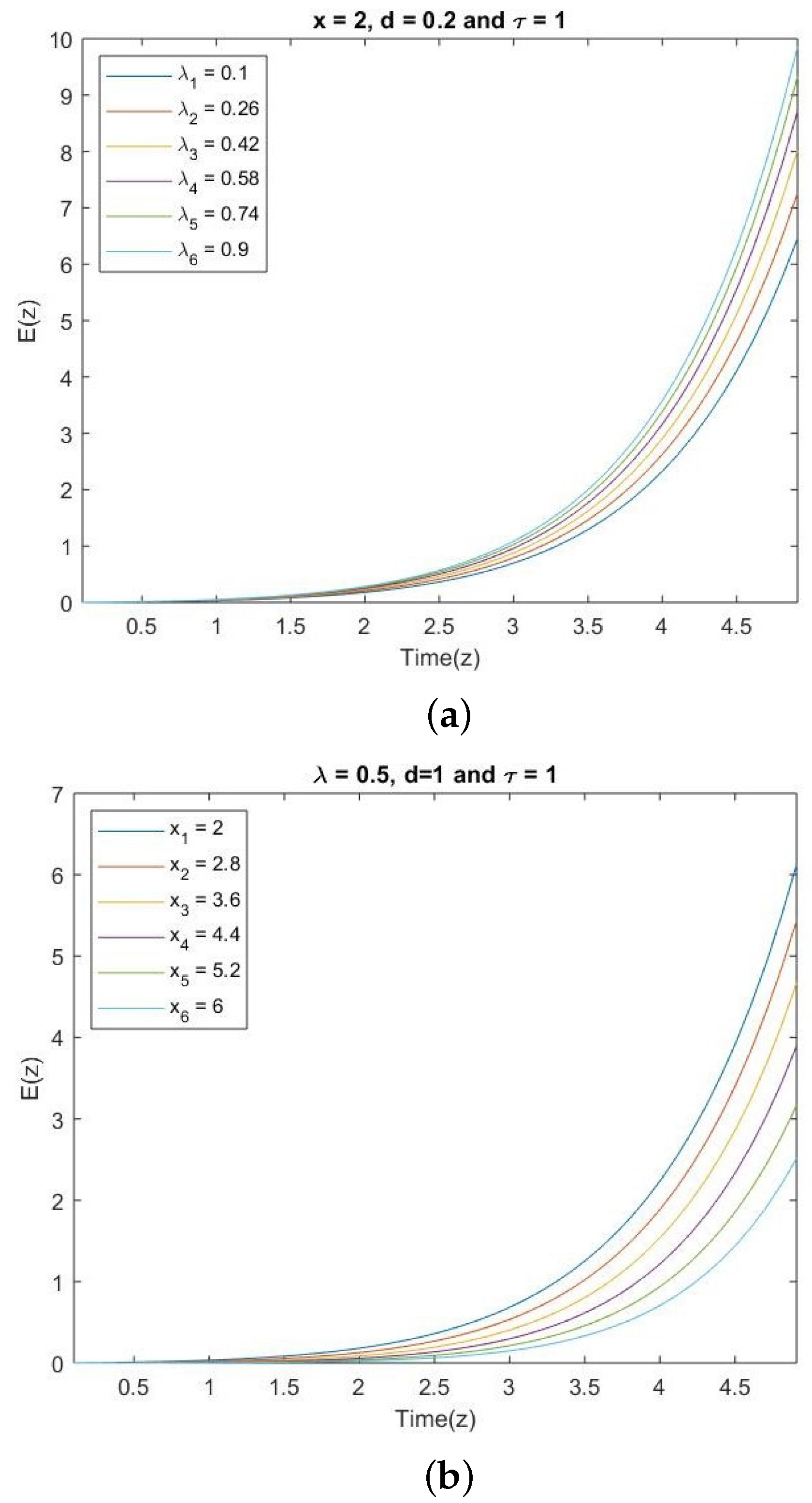
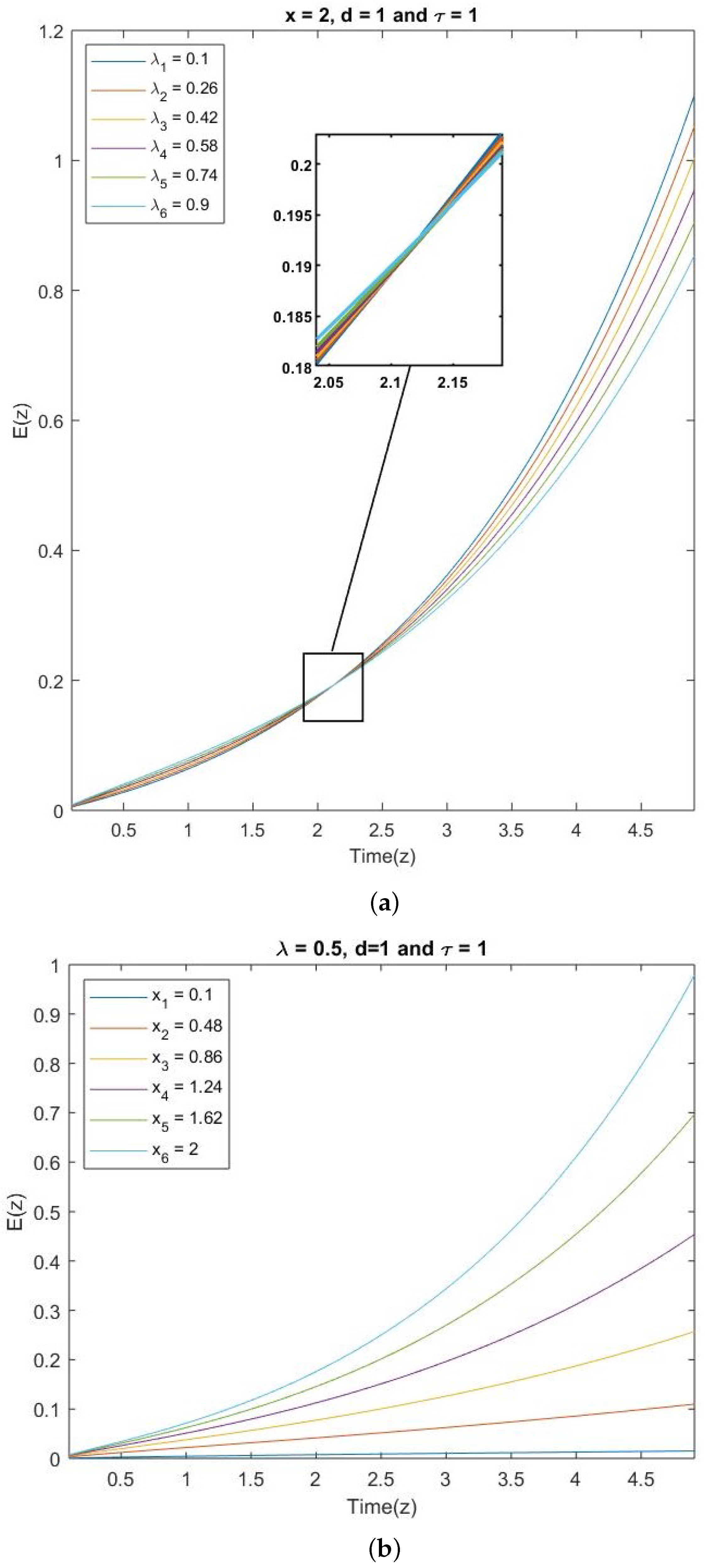
5. Comments on the Graphical Interpretations

Figure 1 depicts the plots of solutions to Equation (35) with parametric values ${\mathbf{E}}_0=1,q=20,p=21$, and $z=0.5,\cdots ,5$ for various values of $\lambda =0.1,0.2,\cdots ,0.9$ in Figure 1a and with fixed values of $x=2,d=0.2$, and $\tau =1$. In Figure 1b, we fix the values to $\tau =1,d=1$ and $\lambda =0.5$ and generate graphs for various values of $x=0.1,\cdots ,2$. The valid region of convergence of the solutions is given by the time interval $z=0.5,\cdots ,5$. Figure 2 exhibits 2D plots of the solutions to Equation (43) for various values of $\lambda$ and x in Figure 2a and Figure 2b, respectively, with fixed values of $\tau =1,d=1$, and ${\mathbf{E}}_0=1$. The graphical findings show that the region of convergence of the solutions was continually dependent on the parameters $\lambda$ and x. As a result, evaluating the behavior of the solutions for various parameters and time periods revealed that $\mathbf{E}\left(z\right)$ was always positive. Furthermore, we could change the values of $\lambda ,x,\tau ,$ and d to obtain more accurate results.

6. Conclusions

Because of the usefulness and great importance of the kinetic equation in some astrophysical issues, fractional kinetic equations have been investigated to describe the various phenomena governed by anomalous reactions in dynamical systems [6,7,8,9]. Several authors have recently presented solutions to various families of fractional kinetic equations involving special functions using the Laplace transform, Sumudu transform, Prabhakar-type operators, Hadamard fractional integrals, and pathway-type transform based on these principles (see, for example, [10,11,12,13,14,15,16,17,18,19,20,21,22,23,24,25]).

Motivated by the above works, the authors developed a new and generalized form of the fractional kinetic equation involving the generalized incomplete Wright hypergeometric function. This new generalization can be used to compute the change in chemical composition in stars such as the Sun. The manifold generality of the Mittag-Leffler function was discussed in terms of the solution to the above fractional kinetic equation by applying a pathway-type transform. Furthermore, a graphical representation of the solutions was provided to demonstrate the behavior of these solutions and to analyze special situations for fractional kinetic equations.

References

1. Abbas, S.; Benchohra, M.; Guerekata, G.M.N. Topics in Fractional Differential Equations; Springer: New York, NY, USA, 2012. [Google Scholar]
2. Zhou, Y. Basic Theory of Fractional Differential Equations; World Scientific: Singapore, 2014. [Google Scholar]
3. Abbas, M.I.; Ragusa, M.A. Solvability of Langevin equations with two Hadamard fractional derivatives via Mittag-Leffler functions. Appl. Anal. 2020, 101, 3231–3245. [Google Scholar]
4. Bakhet, A.; He, F. On the matrix version of extended Struve function and its application on fractional calculus. Filomat 2022, 36, 3381–3392. [Google Scholar] [CrossRef]
5. Youssri, Y.H.; Abd-Elhameed, W.M.; Ahmed, H.M. New fractional derivative ex-pression of the shifted third-kind Chebyshev polynomials: Application to a type of non-linear fractional pantograph differential equations. J. Funct. Spaces 2022, 3966135. [Google Scholar]
6. Saxena, R.K.; Mathai, A.M.; Haubold, H.J. On fractional kinetic equations. Astrophys. Space Sci. 2002, 282, 281–287. [Google Scholar] [CrossRef]
7. Saxena, R.K.; Mathai, A.M.; Haubold, H.J. On generalized fractional kinetic equations. Phys. A 2004, 344, 657–664. [Google Scholar]
8. Saxena, R.K.; Kalla, S.L. On the solutions of certain fractional kinetic equations. Appl. Math. Comput. 2008, 199, 504–511. [Google Scholar] [CrossRef]
9. Chaurasia, V.B.L.; Pandey, S.C. On the new computable solution of the generalized fractional kinetic equations involving the generalized function for the fractional calculus and related functions. Astrophys. Space Sci. 2008, 317, 213–219. [Google Scholar] [CrossRef]
10. Kolokoltsov, V.N.; Troeva, M. A new approach to fractional kinetic evolutions. Fractal Fract. 2022, 6, 49. [Google Scholar] [CrossRef]
11. Haubold, H.J.; Mathai, A.H. The fractional kinetic equation and thermonuclear functions. Astrophys. Space Sci. 2000, 327, 53–63. [Google Scholar] [CrossRef]
12. Habenom, H.; Oli, A.; Suthar, D.L. (p, q)-Extended Struve function: Fractional integrations and application to fractional kinetic equations. J. Math. 2021, 2021, 5536817. [Google Scholar]
13. Sharma, K.P.; Bhargava, A.; Suthar, D.L. Application of the Laplace transform to a new form of fractional kinetic equation involving the composition of the Galue Struve function and the Mittageffler function. Math. Probl. Eng. 2022, 2022, 5668579. [Google Scholar] [CrossRef]
14. Khan, O.; Khan, N.; Choi, J.; Nisar, K.S. A type of fractional Kinetic equations associated with the (p, q)-extented τ-hypergeomtric and confluent hypergeomtric functions. Nonlinear Funct. Anal. Appl. 2021, 26, 381–392. [Google Scholar]
15. Hidan, M.; Akel, M.; Abd-Elmageed, H.; Abdalla, M. Solution of fractional kinetic equations involving extended (k, t)-Gauss hypergeometric matrix functions. AIMS Math. 2022, 7, 14474–14491. [Google Scholar] [CrossRef]
16. Abubakar, U.M. Solutions of fractional kinetic equations using the (p, q; l)-extended τ -Gauss hypergeometric function. J. New Theory 2022, 38, 25–33. [Google Scholar] [CrossRef]
17. Purohit, S.D.; Ucar, F. An application of q-Sumudu transform for fractional q-kinetic equation. Turk. J. Math. 2018, 42, 726–734. [Google Scholar] [CrossRef]
18. Agarwal, P.; Ntouyas, S.K.; Jain, S.; Chand, M.; Singh, G. Fractional kinetic equations involving generalized k-Bessel function via Sumudu transform. Alex. Eng. J. 2018, 57, 1937–1942. [Google Scholar] [CrossRef]
19. Yagci, O.; Sahin, R. Solutions of fractional kinetic equations involving generalized Hurwitz-Lerch Zeta functions using Sumudu transform. Commun. Fac. Sci. Univ. Ank. Ser. A1 Math. Stat. 2021, 70, 678–689. [Google Scholar] [CrossRef]
20. Akel, M.; Hidan, M.; Boulaaras, S.; Abdalla, M. On the solutions of certain fractional kinetic matrix equations involving Hadamard fractional integrals. AIMS Math. 2022, 7, 15520–15531. [Google Scholar] [CrossRef]
21. Ahmed, W.; Salamoon, A.; Pawar, D. Solution of fractional kinetic equation for Hadamard type fractional integral via Mellin transform. Gulf. J. Math. 2022, 12, 15–27. [Google Scholar] [CrossRef]
22. Abdalla, M.; Akel, M. Contribution of using Hadamard fractional integral operator via Mellin integral transform for solving certain fractional kinetic matrix equations. Fractal Fract. 2022, 6, 305. [Google Scholar] [CrossRef]
23. Kumar, D. Solution of fractional kinetic equation by a class of integral transform of pathway type. J. Math. Phys. 2013, 54, 043509. [Google Scholar] [CrossRef]
24. Mathur, G.A.R. Solution of fractional kinetic equations by using integral transform. AIP Conf. Proc. 2020, 2253, 020004. [Google Scholar]
25. Dorrego, G.A.; Kumar, D. A generalization of the kinetic equation using the Prabhakar-type operators. Honam Math. J. 2017, 39, 401–416. [Google Scholar]
26. Chaudhry, M.A.; Zubair, S.M. On a Class of Incomplete Gamma Functions with Applications; Chapman and Hall/CRC: Boca Raton, FL, USA, 2002. [Google Scholar]
27. Virchenko, N.; Kalla, S.L.; Al-Zamel, A. Some results on a generalized hypergeometric function. Integral Transforms Spec. Funct. 2001, 12, 89–100. [Google Scholar] [CrossRef]
28. Nisar, K.S.; Rahman, G.; Mubeen, S.; Arshad, M. The incomplete Pochhammer symbols and their application to generalized hypergeometric functions. Int. Bull. Math. Res. 2017, 4, 1–13. [Google Scholar]
29. Khan, N.; Usman, T.; Aman, M.; Al-Omari, S.; Araci, S. Computation of certain integral formulas involving generalized Wright function. Adv. Differ. Equ. 2020, 1–10. [Google Scholar] [CrossRef]
30. Ghaffar, A.; Saif, A.; Iqbal, M.; Rizwan, M. Two classes of integrals involving extended Wright type generalized hypergeometric function. Commun. Math. Appl. 2019, 10, 599–606. [Google Scholar] [CrossRef]
31. Srivastava, H.M.; Chaudhry, M.A.; Agarwal, R.P. The incomplete Pochhammer symbols and their applications to hypergeometric and related functions. Integral Transform. Spec. Funct. 2012, 23, 659–683. [Google Scholar] [CrossRef]
Figure 1. Graphs of the solution to Equation (35) with various values of λ in (a) and various values of x in (b).
Fractalfract 07 00348 g001
Figure 2. Graphs of the solution to Equation (43) with various values of λ in (a) and various values of x in (b).
Fractalfract 07 00348 g002
Disclaimer/Publisher’s Note: The statements, opinions and data contained in all publications are solely those of the individual author(s) and contributor(s) and not of MDPI and/or the editor(s). MDPI and/or the editor(s) disclaim responsibility for any injury to people or property resulting from any ideas, methods, instructions or products referred to in the content.