Synchronization in Finite Time of Fractional-Order Complex-Valued Delayed Gene Regulatory Networks

Abstract

The synchronization in finite time of fractional-order complex-valued gene networks with time delays is studied in this paper. Several sufficient conditions of the synchronization in finite time for the relevant network models are explored based on feedback controllers and adaptive controllers. Then, the setting time of the response is estimated by the theory of fractional calculus. Finally, to validate the theoretical results, a numerical example is presented using the proposed two controllers, showing that the setting time based on the adaptive controller is shorter than the that based on the feedback controller.

1. Introduction

Gene regulatory networks control gene expression and describe the relationship between deoxyribonucleic acid, ribonucleic acid, and small molecules in organisms. The abundance of the gene product leads to the aggregation of the molecular types of action between them, playing an essential role in the cycle, differentiation, metabolic processes, and signal transduction of cells, which are controlled by gene networks [1]. There are numerous gene regulatory network models, including linear models [2,3], Bayesian networks [4,5], neural networks [6], differential equations [7], and models including stochastic components at the molecular level [8,9]. In recent decades, the extensive application of gene regulatory networks has been explored in various areas, such as biotechnological practices [10,11,12], integrated networks [13,14], and mechanical systems [15,16].

As is well known, fruitful results based on the gene network of integer-order differential equations have been reported [17,18,19]. With the development of the theory of fractional-order calculus and fractional-order differential equations [20,21,22,23], various applications of gene regulatory networks that employ fractional-order calculus, such as the fields of medical science, control, and biotechnology, have shown distinct advantages due to the merits of memory and heredity properties, see [24,25,26] and the references therein. In [24], the results indicated that the most significant benefit of using gene regulatory networks with fractional orders for their memorability and hereditary properties is the enhancement in the dexterity and accuracy of models. The authors found that by combining fractional derivatives, the basic computing power of gene regulatory networks can be enhanced and the processing of various signals can be efficiently processed [25]. In [26], the authors extended the general form of the Lyapunov–Krasovskii function to a new fractional form and derived the stability criteria for gene regulatory network systems with time delays and fractional-order dynamics.

Generally speaking, the time delays, which are usually caused by oscillation, instability, and other poor performance, unavoidably exist in most dynamical networks [27,28,29,30,31], including gene networks [32], neural networks [33,34,35,36], and evolutionary dynamics. As for the gene network models, there always exists certain time delays in the expression of most genes due to the fact that these genes and their regulatory interactions are usually not implemented immediately. It should be noted that, recently, the research interest has been transferring from traditional real-valued gene regulatory networks to complex-valued models. This is because complex-valued gene networks with complex numbers for various parameters [37] are more practical when compared with real-valued networks. Nowadays, complex-valued gene regulatory networks with fractional order are profoundly studies and many excellent results have been found, such as projective multi-synchronization [38] and global synchronization [39]. However, most of the methods in these works are based on separating the complex-valued system into two real-valued systems, which leads to a more tedious proof process and increases the complexity of the algorithm. Hence, it is important to study fractional-order complex-valued gene regulatory networks directly in the complex field [40,41,42].

Synchronization plays a prominent role in the dynamical behaviors of gene regulatory networks, which has increasingly attracted experts’ interests [43,44,45]. Two or more systems communicating among gene molecules to realize a synergistic behavior and to adjust their dynamic characteristics is called synchronization of gene regulatory network. Due to the extensive application of synchronization in information processing, it has developed rapidly [46,47,48]. In [47], by using Lyapunov stability, the synchronization and asymptotic stability of a sort of fractional-order gene regulatory network were studied. Furthermore, in [48], through the designed adaptive controller, the gene regulatory network synchronization problem of fractional order was analyzed.

Inspired by the above description, this paper aims to analyze the problem of synchronization in finite time of fractional-order complex-valued gene regulatory networks. Analyzing complex-valued gene regulatory networks is more challenging than analyzing real-valued models. The chief contributions are summarized as follows:

•

To analyze the synchronization in finite time for the addressed models, two different controllers are designed to achieve a flexible control of synchronization.

•

The presented complex-valued gene regulatory networks are implemented as an entirety form without any decomposition.

•

A novel complex-valued sign function is employed to design the adaptive controller to achieve a more efficient control strategy for the problem of synchronization in finite time.

The article is structured as follows: Section 2 presents the Riemann–Liouville integral and Caputo fractional derivative, introduces appropriate symbolic functions of the complex number field, and cites some complex-number-related lemmas. Section 3 introduces models of gene regulatory networks. In Section 4 and Section 5, two controllers are presented and two theorems regarding synchronization in finite time of complex-valued gene regulatory networks are given. Section 6 provides a numerical example to demonstrate the feasibility and effectiveness of the theoretical results. Finally, the article concludes with a summary.

Notations: ${\mathbb{R}}^n$ and ${\mathbb{C}}^n$ denote the collection of n-dimensional real-valued and complex-valued vectors, respectively. ı denotes the imaginary unit. For any $z\in \mathbb{C}$, Re$\left(z\right)$ represents the real part of z and Im$\left(z\right)$ represents the imaginary part. $\overline{z}$ is the conjugate of z; ${\left|z\right|}_1=\left|\mathrm{Re}\left(z\right)\right|+\left|\mathrm{Im}\left(z\right)\right|$, and ${\left|z\right|}_2=\sqrt{z\overline{z}}$. For any $z\in {\mathbb{C}}^n$, ${\parallel z\parallel }_1={\sum }_{k=1}^n{\left|z_i\right|}_1$, ${\parallel z\parallel }_2=\sqrt{{\sum }_{k=1}^n{\left|z_i\right|}_2^2}$.

2. Preliminaries

Definition 1

([49]). For a function $\phi \left(t\right):[0,+\infty ]\to \mathbb{C}$, the Riemann–Liouville fractional integral is described as

$${}_0^{RL}{D}_t^{\alpha }\phi \left(t\right)=\frac{1}{\Gamma \left(\alpha \right)}{\int }_0^t{(t-\varsigma )}^{\alpha -1}\phi \left(\varsigma \right)d\varsigma ,$$

where $0<\alpha <1$ and $\Gamma \left(\alpha \right)={\int }_0^{+\infty }{\displaystyle \frac{t^{\alpha -1}}{e^{\mu }}}d\mu$.

Definition 2

([49]). For a function $\phi \left(t\right):[0,+\infty ]\to \mathbb{C}$, the Caputo fractional derivative is defined by

$$\begin{array}{c}\hfill {}_0^C{D}_t^{\alpha }\phi \left(t\right)=\frac{1}{\Gamma (1-\alpha )}{\int }_0^t{(t-\varsigma )}^{-\alpha }{\phi }^{\prime }\left(\varsigma \right)d\varsigma .\end{array}$$

where $\alpha \in (0,1)$.

Lemma 1

([50]). For any $\alpha \in \mathbb{C}$, $\beta \in \mathbb{C}$, and for any positive number $\eta \in \mathbb{R}$, it holds that

$$\alpha \overline{\beta }+\overline{\alpha }\beta \le \eta \alpha \overline{\alpha }+\frac{1}{\eta }\beta \overline{\beta }.$$

Definition 3

([41]). $\forall z\left(t\right)\in \mathbb{C}$, the symbolic functions in complex fields is defined as

$$\left[z\right(t\left)\right]=\mathrm{sign}\left(\mathrm{Re}\right(z\left(t\right)\left)\right)+\mathrm{isign}\left(\mathrm{Im}\right(z\left(t\right)\left)\right).$$

Lemma 2

([41]). $\forall z\left(t\right)\in {\mathbb{C}}^n$, the following three formulas are true.

$$\begin{array}{cc}& \left(i\right)\left[z\left(t\right)\right]\times \overline{z\left(t\right)}+\overline{\left[z\right(t\left)\right]}\times z\left(t\right)={2\left|z\left(t\right)\right|}_1\ge 2{\left|z\left(t\right)\right|}_2,\hfill \\ & \left(ii\right)2_0^C{D}_t^{\alpha }{\left|z\left(t\right)\right|}_1\le \left(\overline{\left[z\right(t\left)\right]}{\times }_0^C{D}_t^{\alpha }z\left(t\right)+\left[z\left(t\right)\right]{\times }_0^C{D}_t^{\alpha }\overline{z\left(t\right)}\right),where0<\alpha <1,\hfill \\ & \left(iii\right)\left[z\left(t\right)\right]\times \overline{\left[z\right(t\left)\right]}=\left|\mathrm{sign}\left(\mathrm{Re}\left(z\left(t\right)\right)\right)\right|+\left|\mathrm{sign}\left(\mathrm{Im}\left(z\left(t\right)\right)\right)\right|={\left|\left[z\left(t\right)\right]\right|}_1.\hfill \end{array}$$

Lemma 3

([41]). For any $\alpha \in \mathbb{C}$, there is

$$\alpha +\overline{\alpha }=2\mathrm{Re}\left(\alpha \right)\le {2\left|\alpha \right|}_2\le 2{\left|\alpha \right|}_1.$$

Lemma 4

([51]). Let analytic function $\phi \left(t\right)\in \mathbb{C}$ be continuous, and for any $\vartheta \in \mathbb{C}$, it holds

$${}_0^C{D}_t^{\alpha }\left((\phi \left(t\right)-\vartheta )\times \left(\overline{\phi \left(t\right)-\vartheta }\right)\right)\le \left(\overline{\phi \left(t\right)-\vartheta }\right)\times {}_0^C{D}_t^{\alpha }\phi \left(t\right)+(\phi \left(t\right)-\vartheta )\times {}_0^C{D}_t^{\alpha }\overline{\phi \left(t\right)},0<\alpha <1.$$

3. System Description

Considering that gene regulatory networks are formed by the interplay of genes, the gene model proposed in this paper is designed as a two-dimensional model, which is written as the following fractional-order differential equations:

$$\left\{\begin{array}{cc}\hfill {}_0^C{D}_t^{\alpha }{\phi }_i\left(t\right)& =-a_i{\phi }_i\left(t\right)+\sum _{j=1}^n{\omega }_{ij}{\zeta }_j\left({\varphi }_j(t-{\tau }_1)\right)+B_i,\hfill \\ \hfill {}_0^C{D}_t^{\alpha }{\varphi }_i\left(t\right)& =-c_i{\varphi }_i\left(t\right)+d_i{\phi }_i(t-{\tau }_2),i\in {\mathbb{N}}^{+}\hfill \end{array}\right.$$

(1)

for $\alpha \in (0,1)$, $t⩾0$, where ${\phi }_i\left(t\right)$, ${\varphi }_i\left(t\right)$ represent the density of the ith messenger RNA as well as protein at t. The degradation rate of messenger RNA and protein are denoted by $a_i$ and $c_i$, respectively. $d_i>0$ describes the translation rate. ${\tau }_1$ and ${\tau }_2$ correspond to the delay in different gene transcription processes. ${\omega }_{ij}$ represents the coupling relations of the complex-valued system, which is depicted as follows:

$${\omega }_{ij}=\left\{\begin{array}{cc}\hfill b_{ij},& theactivatingfactorofgeneiistranscriptionfactorj;\hfill \\ \hfill 0,& thereisnoconnectionbetweenjandi;\hfill \\ \hfill -b_{ij},& theantirepressorofgeneiistranscriptionfactorj.\hfill \end{array}\right.$$

(2)

$B_i={\sum }_{j\in I_i}{b}_{ij}$, where $b_{ij}$ are the transcriptional rates of factor j to i which are bounded constants and have no units of measure and $I_i$ is a repressor of gene i that is the aggregate of all values of j. $\zeta \left({\varphi }_j\left(t\right)\right)$ is referred to as the feedback regulation of transcription by proteins, which is described as follows:

$$\zeta \left({\varphi }_j\left(t\right)\right)={\displaystyle \frac{{({\varphi }_j\left(t\right)/{\beta }_j)}^{{\Theta }_j}}{{({\varphi }_j\left(t\right)/{\beta }_j)}^{{\Theta }_j}+1}},$$

(3)

where ${\Theta }_j$ means the Hill coefficient and ${\beta }_j>0$ describes the constant. Obviously, ${\zeta }_j\left({\varphi }_j\left(t\right)\right)$ is a monotonically increasing function. In addition, the initial conditions are ${\phi }_i\left(s\right)={\delta }_i^{\left(1\right)}\left(s\right),s\in [-{\tau }_1,0]$, ${\varphi }_i\left(s\right)={\gamma }_i^{\left(1\right)}\left(s\right)$, and $s\in [-{\tau }_2,0]$.

The corresponding response system of model (1) is depicted as

$$\left\{\begin{array}{cc}\hfill {}_0^C{D}_t^{\alpha }{\kappa }_i\left(t\right)& =-a_i{\kappa }_i\left(t\right)+\sum _{j=1}^n{\omega }_{ij}{\zeta }_j\left({\psi }_j(t-{\tau }_1)\right)+B_i+u_i\left(t\right),\hfill \\ \hfill {}_0^C{D}_t^{\alpha }{\psi }_i\left(t\right)& =-c_i{\psi }_i\left(t\right)+d_i\kappa (t-{\tau }_2)+\widetilde{u_i}\left(t\right),i\in {\mathbb{N}}^{+},\hfill \end{array}\right.$$

(4)

where the messenger RNA and protein concentrations of the system (4) are denoted by ${\kappa }_i\left(t\right),{\psi }_i\left(t\right)$, and $t⩾0$. The system (4) and the system (1) have identical coefficients. $u_i\left(t\right)$ and $\widetilde{u_i}\left(t\right)$ stand for the designed controller which will be given later, and the initial values of the model (4) are given by ${\kappa }_i\left(s\right)={\delta }_i^{\left(2\right)}\left(s\right)$, $s\in [-{\tau }_1,0],$ ${\psi }_i\left(s\right)={\gamma }_i^{\left(2\right)}\left(s\right)$, and $s\in [-{\tau }_2,0].$

Let ${\varrho }_{\phi i}\left(t\right)={\kappa }_i\left(t\right)-{\phi }_i\left(t\right)$, and ${\varrho }_{\varphi i}\left(t\right)={\psi }_i\left(t\right)-{\varphi }_i\left(t\right)$, then the following error systems are obtained

$$\left\{\begin{array}{cc}\hfill {}_0^C{D}_t^{\alpha }{\varrho }_{\phi i}\left(t\right)& =-a_i{\varrho }_{\phi i}\left(t\right)+\sum _{j=1}^n{\omega }_{ij}{\zeta }_j\left({\varrho }_{\varphi j}(t-{\tau }_1)\right)+u_i\left(t\right),\hfill \\ \hfill {}_0^C{D}_t^{\alpha }{\varrho }_{\varphi i}\left(t\right)& =-c_i{\varrho }_{\varphi i}\left(t\right)+d_i{\varrho }_{\phi i}(t-{\tau }_2)+\widetilde{u_i}\left(t\right),t⩾0,\hfill \end{array}\right.$$

(5)

with initial conditions

$$\left\{\begin{array}{cc}\hfill {\varrho }_{\phi i}\left(s\right)=& {\delta }_i\left(s\right),s\in [-{\tau }_1,0],\hfill \\ \hfill {\varrho }_{\varphi i}\left(s\right)=& {\gamma }_i\left(s\right),s\in [-{\tau }_2,0],\hfill \end{array}\right.$$

(6)

where ${\zeta }_j\left({\varrho }_{\varphi j}(t-{\tau }_1)\right)={\zeta }_j\left({\psi }_j(t-{\tau }_1)\right)-{\zeta }_j\left({\varphi }_j(t-{\tau }_1)\right)$, $i\in {\mathbb{N}}^{+}$.

Definition 4

([52]). If there exists a setting time $T\ge 0$ such that ${lim}_{t\to T}\left(\right||{\varrho }_{\phi }{\left(t\right)\left|\right|}_i+\left|\right|{\varrho }_{\varphi }{\left(t\right)\left|\right|}_i)=0$ and $\left|\right|{\varrho }_{\phi }{\left(t\right)\left|\right|}_i+\left|\right|{\varrho }_{\varphi }\left(t\right){\left|\right|}_i\equiv 0$, $\forall t\ge T$,$i=1,2$, then the driving system (1) is synchronized in finite time with the response system (4).

In this paper, it is necessary to make the following assumptions.

Assumption 1.

For any $u,v\in \mathbb{C}$, there exists a real number $l_j>0$ such that

$$|{\zeta }_j\left(u\right)-{\zeta }_j{\left(v\right)|}_i⩽l_j{|u-v|}_i,i,j\in {\mathbb{N}}^{+}.$$

(7)

Assumption 2.

In model (5), the initial values satisfy

$$\begin{array}{cc}\hfill & {\left|\right|\delta \left(s\right)\left|\right|}_1=\underset{-{\tau }_1\le s\le 0}{sup}\sum _{i=1}^n|{\delta }_i{\left(s\right)|}_2\le \sum _{i=1}^n|{\delta }_i\left(0\right){|}_2,s\in [-{\tau }_1,0]),\hfill \\ \hfill & {\left|\right|\gamma \left(s\right)\left|\right|}_1=\underset{-{\tau }_2\le s\le 0}{sup}\sum _{i=1}^n|{\gamma }_i{\left(s\right)|}_2\le \sum _{i=1}^n|{\gamma }_i\left(0\right){|}_2,s\in [-{\tau }_2,0]).\hfill \end{array}$$

(8)

4. Synchronization in Finite Time with a Feedback Controller

In this section, in order to establish the criteria of synchronization in finite time, the following complex-valued feedback controller is designed:

$$\left\{\begin{array}{c}{u}_i\left(t\right)=-k_i{\varrho }_{\phi i}\left(t\right)-{\displaystyle \frac{\eta }{\overline{{\varrho }_{\phi i}\left(t\right)}}}{\displaystyle \frac{|{\varrho }_{\phi i}{\left(t\right)|}_2}{\left|\right|{\varrho }_{\phi }\left(t\right){\left|\right|}_2}},\hfill \\ {\tilde{u}}_i\left(t\right)=-{\tilde{k}}_i{\varrho }_{\varphi i}\left(t\right)-{\displaystyle \frac{\tilde{\eta }}{\overline{{\varrho }_{\varphi i}\left(t\right)}}}{\displaystyle \frac{|{\varrho }_{\varphi i}{\left(t\right)|}_2}{\left|\right|{\varrho }_{\varphi }\left(t\right){\left|\right|}_2}},\hfill \end{array}\right.$$

(9)

where $q_i$ and $g_i$ are adaptive coupling strengths and $k_i,{\tilde{k}}_i,\eta ,$ and $\tilde{\eta }$ are arbitrary complex numbers, $i=1,2,...,n$.

Assumption 3.

The parameters of the model (5) and controller (9) satisfy the following conditions

$$a_i+\overline{a_i}+k_i+\overline{k_i}-\sum _{j=1}^n|{\omega }_{ij}{|}^2\ge 0,c_i+\overline{c_i}+\widetilde{k_i}+\overline{\widetilde{k_i}}-{\left|d_i\right|}^2\ge 0.$$

Theorem 1.

Under Assumptions 1–3, the drive system (1) and the response system (4) can achieve synchronization in finite time under the action of the adaptive controller (9). Meanwhile, the time of synchronization is estimated as

$$T_1={\left[{\displaystyle \frac{\Gamma (\alpha +1)\left({\sum }_{i=1}^n\right|{\varrho }_{\phi i}\left(0\right){|}_2^2+{\sum }_{i=1}^n\left|{\varrho }_{\varphi i}\left(0\right){|}_2^2\right)}{2\times \mathrm{Re}(\eta +\tilde{\eta })}}\right]}^{\frac{1}{\alpha }}.$$

Proof 

(Proof of Theorem 1). Consider the following Lyapunov function,

$$V\left(t\right)=\sum _{i=1}^n|{\varrho }_{\phi i}{\left(t\right)|}_2^2+\sum _{i=1}^n{\left|{\varrho }_{\varphi i}\left(t\right)\right|}_2^2.$$

(10)

By calculating the derivative of $V\left(t\right)$ along the error system (5), we can obtain from Lemma 4 that

$$\begin{array}{cc}\hfill & {}_0^C{D}_t^{\alpha }V\left(t\right)\hfill \\ \hfill =& \sum _{i=1}^n{}_0^C{D}_t^{\alpha }|{\varrho }_{\phi i}{\left(t\right)|}_2^2+\sum _{i=1}^n{}_0^C{D}_t^{\alpha }{\left|{\varrho }_{\varphi i}\left(t\right)\right|}_2^2\hfill \\ \hfill =& \sum _{i=1}^n{\varrho }_{\phi i}\left(t\right){[}_0^C{D}_t^{\alpha }\overline{{\varrho }_{\phi i}\left(t\right)}+{\overline{{\varrho }_{\phi i}\left(t\right)}}_0^C{D}_t^{\alpha }{\varrho }_{\phi i}\left(t\right)]+\sum _{i=1}^n{\varrho }_{\varphi i}\left(t\right){[}_0^C{D}_t^{\alpha }\overline{{\varrho }_{\varphi i}\left(t\right)}+{\overline{{\varrho }_{\varphi i}\left(t\right)}}_0^C{D}_t^{\alpha }{\varrho }_{\varphi i}\left(t\right)]\hfill \\ \hfill =& \sum _{i=1}^n{\varrho }_{\phi i}\left(t\right)\left[-\overline{a_i}\overline{{\varrho }_{\phi i}\left(t\right)}-\overline{k_i}\overline{{\varrho }_{\phi i}\left(t\right)}+\sum _{j=1}^n\overline{{\omega }_{ij}}\overline{{\zeta }_j\left({\varrho }_{\varphi j}(t-{\tau }_1)\right)}-{\displaystyle \frac{\eta }{{\varrho }_{\phi i}\left(t\right)}}{\displaystyle \frac{|{\varrho }_{\phi i}{\left(t\right)|}_2}{\left|\right|{\varrho }_{\phi }\left(t\right){\left|\right|}_2}}\right]\hfill \\ \hfill & +\sum _{i=1}^n\overline{{\varrho }_{\phi i}\left(t\right)}\left[-a_i{\varrho }_{\phi i}\left(t\right)-k_i{\varrho }_{\phi i}\left(t\right)+\sum _{j=1}^n{\omega }_{ij}{\zeta }_j\left({\varrho }_{\varphi j}(t-{\tau }_1)\right)-{\displaystyle \frac{\overline{\eta }}{\overline{{\varrho }_{\phi i}\left(t\right)}}}{\displaystyle \frac{|{\varrho }_{\phi i}{\left(t\right)|}_2}{\left|\right|{\varrho }_{\phi }\left(t\right){\left|\right|}_2}}\right]\hfill \\ \hfill & +\sum _{i=1}^n{\varrho }_{\varphi i}\left(t\right)\left[-\overline{c_i}\overline{{\varrho }_{\varphi i}\left(t\right)}-\overline{\widetilde{k_i}}\overline{{\varrho }_{\varphi i}\left(t\right)}+\overline{d_i}\overline{{\varrho }_{\phi i}(t-{\tau }_2)}-{\displaystyle \frac{\tilde{\eta }}{{\varrho }_{\varphi i}\left(t\right)}}{\displaystyle \frac{|{\varrho }_{\varphi i}{\left(t\right)|}_2}{\left|\right|{\varrho }_{\varphi }\left(t\right){\left|\right|}_2}}\right]\hfill \\ \hfill & +\sum _{i=1}^n\overline{{\varrho }_{\varphi i}\left(t\right)}\left[-c_i{\varrho }_{\varphi i}\left(t\right)-\widetilde{k_i}{\varrho }_{\varphi i}\left(t\right)+d_i{\varrho }_{\phi i}(t-{\tau }_2)-{\displaystyle \frac{\overline{\tilde{\eta }}}{\overline{{\varrho }_{\varphi i}\left(t\right)}}}{\displaystyle \frac{|{\varrho }_{\varphi i}{\left(t\right)|}_2}{\left|\right|{\varrho }_{\varphi }\left(t\right){\left|\right|}_2}}\right]\hfill \\ \hfill =& \sum _{i=1}^n\left[-(a_i+\overline{a_i}+k_i+\overline{k_i}){\left|{\varrho }_{\phi i}\left(t\right)\right|}_2^2+\sum _{j=1}^n\left(\overline{{\omega }_{ij}}{\varrho }_{\phi i}\left(t\right)\overline{{\zeta }_j\left({\varrho }_{\varphi j}(t-{\tau }_1)\right)}\right.\right.\hfill \\ \hfill & \left.\left.+{\omega }_{ij}\overline{{\varrho }_{\phi i}\left(t\right)}{\zeta }_j\left({\varrho }_{\varphi j}(t-{\tau }_1)\right)\right)\right]+\sum _{i=1}^n\left[-(c_i+\overline{c_i}+\widetilde{k_i}+\overline{\widetilde{k_i}}){\left|{\varrho }_{\varphi i}\left(t\right)\right|}_2^2\right.\hfill \\ \hfill & \left.+\overline{d_i}\overline{{\varrho }_{\phi i}(t-{\tau }_2)}{\varrho }_{\varphi i}\left(t\right)+d_i{\varrho }_{\phi i}(t-{\tau }_2)\overline{{\varrho }_{\varphi i}\left(t\right)})\right]-2\times \mathrm{Re}(\eta +\tilde{\eta }).\hfill \end{array}$$

(11)

According to Assumption 1 and Lemma 1, it follows that

$$\begin{array}{cc}\hfill & \sum _{i=1}^n\sum _{j=1}^n\left(\overline{{\omega }_{ij}}{\varrho }_{\phi i}\left(t\right)\overline{{\zeta }_j\left({\varrho }_{\varphi j}(t-{\tau }_1)\right)}+{\omega }_{ij}\overline{{\varrho }_{\phi i}\left(t\right)}{\zeta }_j\left({\varrho }_{\varphi j}(t-{\tau }_1)\right)\right)\hfill \\ \hfill & \le \sum _{i=1}^n\sum _{j=1}^n\left({\omega }_{ij}\overline{{\omega }_{ij}}{\varrho }_{\phi i}\left(t\right)\overline{{\varrho }_{\phi i}\left(t\right)}+{\zeta }_j\left({\varrho }_{\varphi j}(t-{\tau }_1)\right)\overline{{\zeta }_j\left({\varrho }_{\varphi j}(t-{\tau }_1)\right)}\right)\hfill \\ \hfill & \le \sum _{i=1}^n\sum _{j=1}^n\left(|{\omega }_{ij}{|}_2^2|{\varrho }_{\phi i}{|}_2^2+l_j^2{\left|{\varrho }_{\varphi i}(t-{\tau }_1)\right|}_2^2\right).\hfill \end{array}$$

(12)

Similarly,

$$\begin{array}{cc}\hfill & \sum _{i=1}^n\left(\overline{d_i}\overline{{\varrho }_{\phi i}(t-{\tau }_2)}{\varrho }_{\varphi i}\left(t\right)+d_i{\varrho }_{\phi i}(t-{\tau }_2)\overline{{\varrho }_{\varphi i}\left(t\right)}\right)\hfill \\ \hfill & \le \sum _{i=1}^n\left(d_i\overline{d_i}{\varrho }_{\varphi i}\left(t\right)\overline{{\varrho }_{\varphi i}\left(t\right)}+{\varrho }_{\phi i}(t-{\tau }_2)\overline{{\varrho }_{\phi i}(t-{\tau }_2)}\right)\hfill \\ \hfill & \le \sum _{i=1}^n|d_i{|}_2^2|{\varrho }_{\varphi i}{\left(t\right)|}_2^2+{\left|{\varrho }_{\phi i}(t-{\tau }_2)\right|}_2^2.\hfill \end{array}$$

(13)

Based on Assumption 2, applying the Razumikhin condition (see pages 55–56 in ref. [53]) yields

$$\begin{array}{cc}\hfill & \sum _{i=1}^n|{\varrho }_{\varphi i}\left(\epsilon \right)|\le \sum _{i=1}^n\left|{\varrho }_{\varphi i}\left(t\right)\right|,t-{\tau }_1\le \epsilon \le t,\hfill \\ \hfill & \sum _{i=1}^n|{\varrho }_{\phi i}\left(\epsilon \right)|\le \sum _{i=1}^n\left|{\varrho }_{\phi i}\left(t\right)\right|,t-{\tau }_2\le \epsilon \le t.\hfill \end{array}$$

(14)

Then, from (12)–(14), we can obtain

$$\begin{array}{cc}\hfill {}_0^C{D}_t^{\alpha }V\left(t\right)\le & -\sum _{i=1}^n\left[\right(a_i+\overline{a_i}+k_i+\overline{k_i}-\sum _{j=1}^n|{\omega }_{ij}{|}_2^2-1\left)\right|{\varrho }_{\phi i}{\left(t\right)|}_2^2\hfill \\ & +\left.(c_i+\overline{c_i}+\widetilde{k_i}+\overline{\widetilde{k_i}}-l_j^2-|d_i{|}_2^2\left)\right|{\varrho }_{\varphi i}{\left(t\right)|}_2^2\right]\hfill \\ \hfill & -2\times \mathrm{Re}(\eta +\tilde{\eta }).\hfill \end{array}$$

(15)

Under Assumption 3, one has

$${}_0^C{D}_t^{\alpha }V\left(t\right)\le -2\times \mathrm{Re}(\eta +\tilde{\eta }),$$

therefore, let $F\left(t\right)$ be a non-negative function which satisfies the following conditions:

$${}_0^C{D}_t^{\alpha }V\left(t\right)+F\left(t\right)=-2\times \mathrm{Re}(\eta +\tilde{\eta }).$$

(16)

Taking the $\alpha$-order integral from 0 to t of Equation (16), it can be converted to

$$\begin{array}{cc}\hfill V\left(t\right)=& V\left(0\right)-{}_0^{RL}{D}_t^{\alpha }F\left(t\right)+{}_0^{RL}{D}_t^{\alpha }\left(-2\times \left(\mathrm{Re}\left(\eta \right)+\mathrm{Re}\left(\tilde{\eta }\right)\right)\right)\hfill \\ \hfill =& V\left(0\right)-{\displaystyle \frac{1}{\Gamma \left(\alpha \right)}}\times {\int }_0^t\left(F\left(s\right)+2\times \left(\mathrm{Re}\left(\eta \right)+\mathrm{Re}\left(\tilde{\eta }\right)\right)\right){(t-s)}^{\alpha -1}ds.\hfill \end{array}$$

(17)

Obviously, $\Gamma \left(\alpha \right)>0$; therefore, ${}_0^{RL}{D}_t^{\alpha }F\left(t\right)\ge 0$ and the following can be obtained:

$$V\left(t\right)\le V\left(0\right)-{\displaystyle \frac{2\times \mathrm{Re}(\eta +\tilde{\eta })}{\Gamma \left(\alpha \right)}}{\int }_0^t{(t-s)}^{\alpha -1}ds=V\left(0\right)-{\displaystyle \frac{\left(2\times \mathrm{Re}(\eta +\tilde{\eta })\right)t^{\alpha }}{\Gamma (\alpha +1)}}.$$

(18)

${(t-s)}^{\alpha -1}F\left(s\right)$$\left(s\in [0,t)\right)$ is a non-negative function. Hence,

$$\begin{array}{cc}\hfill V\left(t\right)& \le V\left(0\right)-{\displaystyle \frac{M_1}{\Gamma \left(\alpha \right)}}{\int }_0^t{(t-s)}^{\alpha -1}ds\hfill \\ \hfill & =V\left(0\right)-{\displaystyle \frac{M_1{t}^{\alpha }}{\Gamma (\alpha +1)}}.\hfill \end{array}$$

(19)

Letting ${\Phi }_1\left(t\right)=V\left(0\right)-{\displaystyle \frac{\left(2\times \mathrm{Re}(\eta +\tilde{\eta })\right)t^{\alpha }}{\Gamma (\alpha +1)}}$ and $\Phi \left(t\right)=0$ yields

$$\begin{array}{cc}\hfill T_1=& {\left[{\displaystyle \frac{V\left(0\right)\Gamma (\alpha +1)}{2\times \mathrm{Re}(\eta +\tilde{\eta })}}\right]}^{\frac{1}{\alpha }}\hfill \\ \hfill =& {\left[{\displaystyle \frac{\left({\sum }_{i=1}^n\right|{\varrho }_{\phi i}\left(0\right){|}_2^2+{\sum }_{i=1}^n\left|{\varrho }_{\varphi i}\left(0\right){|}_2^2\right)\Gamma (\alpha +1)}{2\times \mathrm{Re}(\eta +\tilde{\eta })}}\right]}^{\frac{1}{\alpha }}.\hfill \end{array}$$

(20)

When $t\ge T_1$, we obtain $V\left(t\right)\le {\Phi }_1\left(t\right)\le 0$, $V\left(t\right)$ as a non-negative function. In addition,

$$\begin{array}{cc}\hfill & \sum _{i=1}^n|{\varrho }_{\phi i}{\left(t\right)|}_2+\sum _{i=1}^n{\left|{\varrho }_{\varphi i}\left(t\right)\right|}_2\hfill \\ \hfill \le & \sqrt{\left(\right|{\varrho }_{\phi 1}{|}^2+\cdots +|{\varrho }_{\phi n}{|}^2+|{\varrho }_{\varphi 1}{|}^2+\cdots +|{\varrho }_{\varphi n}{|}^2)(1^2+\cdots +1^2+1^2+\cdots +1^2)}\hfill \\ \hfill =& \sqrt{(\sum _{i=1}^n|{\varrho }_{\phi i}\left(t\right){|}^2+\sum _{i=1}^n{\displaystyle |}{\varrho }_{\varphi i}\left(t\right){{\displaystyle |}}^2)\left(2n\right)}\hfill \\ \hfill =& \sqrt{2n}\sqrt{V\left(t\right)},\hfill \end{array}$$

(21)

which leads to

$$\sum _{i=1}^n|{\varrho }_{\phi i}\left(t\right)|+\sum _{i=1}^n\left|{\varrho }_{\varphi i}\left(t\right)\right|\equiv 0,\forall t\ge T_1.$$

(22)

According to Definition 3, the drive system (1) and the response system (4) can achieve synchronization in finite time under the state feedback controller (9). □

5. Synchronization in Finite Time with Adaptive Controller

Based on a novel complex-valued sign function, a complex-valued adaptive controller is designed by

$$\left\{\begin{array}{c}{u}_i\left(t\right)=-(q_i\left(t\right)+{\theta }_i)\left[{\varrho }_{\phi i}\left(t\right)\right],\hfill \\ \widetilde{u_i}\left(t\right)=-(g_i\left(t\right)+\widetilde{{\theta }_i})\left[{\varrho }_{\varphi i}\left(t\right)\right],\hfill \\ {}_0^C{D}_t^{\alpha }{q}_i\left(t\right)={\delta }_i{\left|\left[{\varrho }_{\phi i}\left(t\right)\right]\right|}_1,\hfill \\ {}_0^C{D}_t^{\alpha }{g}_i\left(t\right)=\widetilde{{\delta }_i}{\left|\left[{\varrho }_{\varphi i}\left(t\right)\right]\right|}_1,\hfill \end{array}\right.$$

(23)

where $q_i\left(t\right)$ and $g_i\left(t\right)$ are complex-valued functions and ${\theta }_i,\widetilde{{\theta }_i},{\delta }_i,{\tilde{\delta }}_i\in \mathbb{C}$, and $i\in {\mathbb{N}}^{+}$.

Assumption 4.

For the parameters of model (5) and controller (23), the following inequalities hold

$$\mathrm{Re}\left(a_i\right)-|\mathrm{Im}\left(a_i\right)|-|d_i{|}_1\ge 0,$$

$$\mathrm{Re}\left(c_i\right)-|\mathrm{Im}\left(c_i\right)|\sum _{j=1}^n{l}_j^2{\left|{\omega }_{ij}\right|}_1\ge 0,$$

$$\mathrm{Re}\left(q_i\right)\ge 0,\mathrm{Re}\left(g_i\right)\ge 0.$$

Theorem 2.

Under the Assumptions 1 and 2 and condition (4), the drive system (1) and the response system (4) can achieve synchronization in finite time under the action of the adaptive controller (23). Moreover, the time of synchronization is estimated as

$$T_2={\left[{\displaystyle \frac{\Gamma (\alpha +1)\left({\displaystyle \sum _{i=1}^n}|{\varrho }_{\phi i}{\left(0\right)|}_1+{\displaystyle \sum _{i=1}^n}{\left|{\varrho }_{\varphi i}\left(0\right)\right|}_1-{\displaystyle \sum _{i=1}^n}\frac{|q_i\left(0\right)-q_i{|}^2}{{\delta }_i}-{\displaystyle \sum _{i=1}^n}\frac{|g_i\left(0\right)-g_i{|}^2}{\widetilde{{\delta }_i}}\right)}{2n\times (\theta +\tilde{\theta }+\overline{{\theta }_i}+\overline{\widetilde{{\theta }_i}})}}\right]}^{\frac{1}{\alpha }}.$$

Proof .

A Lyapunov function is constructed as

$$\begin{array}{cc}\hfill V\left(t\right)=& \sum _{i=1}^n|{\varrho }_{\phi i}{\left(t\right)|}_1+\sum _{i=1}^n{\left|{\varrho }_{\varphi i}\left(t\right)\right|}_1+\sum _{i=1}^n\frac{1}{2{\delta }_i}(q_i\left(t\right)-q_i)\left(\overline{q_i\left(t\right)-q_i}\right)\hfill \\ \hfill & +\sum _{i=1}^n\frac{1}{2\widetilde{{\delta }_i}}(g_i\left(t\right)-g_i)\left(\overline{g_i\left(t\right)-g_i}\right).\hfill \end{array}$$

By calculating the derivative of $V\left(t\right)$ along the error system (5) with adaptive controller (23), we can obtain from Lemmas 2 and 4 that

$$\begin{array}{cc}\hfill {}_0^C& D_t^{\alpha }V\left(t\right)\hfill \\ \hfill =& \sum _{i=1}^n{}_0^C{D}_t^{\alpha }|{\varrho }_{\phi i}{\left(t\right)|}_1+\sum _{i=1}^n{}_0^C{D}_t^{\alpha }{\left|{\varrho }_{\varphi i}\left(t\right)\right|}_1+\sum _{i=1}^n{}_0^C{D}_t^{\alpha }\left(\frac{1}{2{\delta }_i}(q_i\left(t\right)-q_i)\left(\overline{q_i\left(t\right)-q_i}\right)\right)\hfill \\ \hfill & +\sum _{i=1}^n{}_0^C{D}_t^{\alpha }\left(\frac{1}{2\widetilde{{\delta }_i}}(g_i\left(t\right)-g_i)\left(\overline{g_i\left(t\right)-g_i}\right)\right)\hfill \\ \hfill \le & \frac{1}{2}\sum _{i=1}^n\left({\overline{\left[{\varrho }_{\phi i}\left(t\right)\right]}}_0^C{D}_t^{\alpha }{\varrho }_{\phi i}\left(t\right)+{\left[{\varrho }_{\phi i}\left(t\right)\right]}_0^C{D}_t^{\alpha }\overline{{\varrho }_{\phi i}\left(t\right)}+{\overline{\left[{\varrho }_{\varphi i}\left(t\right)\right]}}_0^C{D}_t^{\alpha }{\varrho }_{\varphi i}\left(t\right)+{\left[{\varrho }_{\varphi i}\left(t\right)\right]}_0^C{D}_t^{\alpha }\overline{{\varrho }_{\varphi i}\left(t\right)}\right)\hfill \\ \hfill & +\frac{1}{2}\sum _{i=1}^n\frac{1}{{\delta }_i}\times \left({(q_i\left(t\right)-q_i)}_0^C{D}_t^{\alpha }\overline{q_i\left(t\right)}+{\left(\overline{q_i\left(t\right)-q_i}\right)}_0^C{D}_t^{\alpha }{q}_i\left(t\right))\right)\hfill \\ \hfill & +\frac{1}{2}\sum _{i=1}^n\frac{1}{\widetilde{{\delta }_i}}\times \left({(g_i\left(t\right)-g_i)}_0^C{D}_t^{\alpha }\overline{g_i\left(t\right)}+{\left(\overline{g_i\left(t\right)-g_i}\right)}_0^C{D}_t^{\alpha }{g}_i\left(t\right))\right)\hfill \\ \hfill =& \frac{1}{2}\sum _{i=1}^n\overline{\left[{\varrho }_{\phi i}\left(t\right)\right]}\left(-a_i{\varrho }_{\phi i}\left(t\right)+\sum _{j=1}^n{\omega }_{ij}{\zeta }_j\left({\varrho }_{\varphi j}(t-{\tau }_1)\right)-q_i\left(t\right)\left[{\varrho }_{\phi i}\left(t\right)\right]-{\theta }_i\left[{\varrho }_{\phi i}\left(t\right)\right]\right)\hfill \\ \hfill & +\frac{1}{2}\sum _{i=1}^n\left[{\varrho }_{\phi i}\left(t\right)\right]\left(\overline{-a_i}\overline{{\varrho }_{\phi i}\left(t\right)}+\sum _{j=1}^n\overline{{\omega }_{ij}}\overline{{\zeta }_j\left({\varrho }_{\varphi j}(t-{\tau }_1)\right)}-\overline{q_i\left(t\right)}\overline{\left[{\varrho }_{\phi i}\left(t\right)\right]}-\overline{{\theta }_i}\overline{\left[{\varrho }_{\phi i}\left(t\right)\right]}\right)\hfill \\ \hfill & +\frac{1}{2}\sum _{i=1}^n\overline{\left[{\varrho }_{\varphi i}\left(t\right)\right]}\left(-c_i{\varrho }_{\varphi i}\left(t\right)+d_i{\varrho }_{\phi i}(t-{\tau }_2)-g_i\left(t\right)\left[{\varrho }_{\varphi i}\left(t\right)\right]-\widetilde{{\theta }_i}\left[{\varrho }_{\varphi i}\left(t\right)\right]\right)\hfill \\ \hfill & +\frac{1}{2}\sum _{i=1}^n\left[{\varrho }_{\varphi i}\left(t\right)\right]\left(\overline{-c_i}\overline{{\varrho }_{\varphi i}\left(t\right)}+\overline{d_i}\overline{{\varrho }_{\phi i}(t-{\tau }_2)}-\overline{g_i\left(t\right)}\overline{\left[{\varrho }_{\varphi i}\left(t\right)\right]}-\widetilde{{\theta }_i}\overline{\left[{\varrho }_{\varphi i}\left(t\right)\right]}\right)\hfill \\ \hfill & +\frac{1}{2}\sum _{i=1}^n\left(\frac{1}{{\delta }_i}(q_i\left(t\right)-q_i){\delta }_i|\left[{\varrho }_{\phi i}\left(t\right)\right]{|}_1+{\frac{1}{\delta }}_i\left(\overline{q_i\left(t\right)-q_i}\right){\delta }_i|\left[{\varrho }_{\phi i}\left(t\right)\right]{|}_1\right)\hfill \\ \hfill & +\frac{1}{2}\sum _{i=1}^n\left(\frac{1}{\widetilde{{\delta }_i}}(g_i\left(t\right)-g_i)\widetilde{{\delta }_i}|\left[{\varrho }_{\varphi i}\left(t\right)\right]{|}_1+\frac{1}{\widetilde{{\delta }_i}}\left(\overline{g_i\left(t\right)-g_i}\right)\widetilde{{\delta }_i}|\left[{\varrho }_{\varphi i}\left(t\right)\right]{|}_1\right)\hfill \\ \hfill =& -\frac{1}{2}\sum _{i=1}^n\left(a_i\left[\overline{{\varrho }_{\phi i}\left(t\right)}\right]{\varrho }_{\phi i}\left(t\right)+\overline{a_i}\left[{\varrho }_{\phi i}\left(t\right)\right]\overline{{\varrho }_{\phi i}\left(t\right)}\right)\hfill \\ \hfill & +\frac{1}{2}\sum _{i=1}^n\sum _{j=1}^n\left({\omega }_{ij}\left[\overline{{\varrho }_{\phi i}\left(t\right)}\right]{\zeta }_j\left({\varrho }_{\varphi j}(t-{\tau }_1)\right)+\overline{{\omega }_{ij}}\left[{\varrho }_{\phi i}\left(t\right)\right]\overline{{\zeta }_j\left({\varrho }_{\varphi j}(t-{\tau }_1)\right)}\right)\hfill \\ \hfill & -\frac{1}{2}\sum _{i=1}^n(q_i\left(t\right)+\overline{q_i\left(t\right)}+{\theta }_i+\overline{{\theta }_i})\left[\overline{{\varrho }_{\phi i}\left(t\right)}\right]\left[{\varrho }_{\phi i}\left(t\right)\right]\hfill \\ \hfill & -\frac{1}{2}\sum _{i=1}^n\left(c_i\left[\overline{{\varrho }_{\varphi i}\left(t\right)}\right]{\varrho }_{\varphi i}\left(t\right)+\overline{c_i}\left[{\varrho }_{\varphi i}\left(t\right)\right]\overline{{\varrho }_{\varphi i}\left(t\right)}\right)\hfill \\ \hfill & +\frac{1}{2}\sum _{i=1}^n\sum _{j=1}^n\left(d_i\left[\overline{{\varrho }_{\varphi i}\left(t\right)}\right]{\varrho }_{\phi i}(t-{\tau }_2)+\overline{d_i}\left[{\varrho }_{\varphi i}\left(t\right)\right]\overline{{\varrho }_{\phi i}(t-{\tau }_2)}\right)\hfill \\ \hfill & -\frac{1}{2}\sum _{i=1}^n(g_i\left(t\right)+\overline{g_i\left(t\right)}+\widetilde{{\theta }_i}+\overline{\widetilde{{\theta }_i}})\left[\overline{{\varrho }_{\varphi i}\left(t\right)}\right]\left[{\varrho }_{\varphi i}\left(t\right)\right]\hfill \\ \hfill & +\frac{1}{2}\sum _{i=1}^n\left((q_i\left(t\right)-q_i)|\left[\overline{{\varrho }_{\phi i}\left(t\right)}\right]{|}_1+\left(\overline{q_i\left(t\right)-q_i}\right)|\left[{\varrho }_{\phi i}\left(t\right)\right]{|}_1\right)\hfill \\ \hfill & +\frac{1}{2}\sum _{i=1}^n\left((g_i\left(t\right)-g_i)|\left[\overline{{\varrho }_{\varphi i}\left(t\right)}\right]{|}_1+\left(\overline{g_i\left(t\right)-g_i}\right)|\left[{\varrho }_{\varphi i}\left(t\right)\right]{|}_1\right),\hfill \end{array}$$

(24)

which, by Lemma 3, gives

$$\begin{array}{cc}\hfill -& \frac{1}{2}\sum _{i=1}^n\left(a_i\left[\overline{{\varrho }_{\phi i}\left(t\right)}\right]{\varrho }_{\phi i}\left(t\right)+\overline{a_i}\left[{\varrho }_{\phi i}\left(t\right)\right]\overline{{\varrho }_{\phi i}\left(t\right)}\right)\hfill \\ \hfill =& \sum _{i=1}^n(-\mathrm{Re}\left(a_i\right)|{\varrho }_{\phi i}\left(t\right){|}_1-\mathrm{Im}\left(a_i\right)\times \hfill \\ \hfill & \left(\mathrm{sign}\left(\mathrm{Im}\left({\varrho }_{\phi i}\left(t\right)\right)\right)\times \mathrm{Re}\left({\varrho }_{\phi i}\left(t\right)\right)-\mathrm{sign}(\mathrm{Re}\left({\varrho }_{\phi i}\left(t\right)\right)\times \mathrm{Im}\left({\varrho }_{\phi i}\left(t\right)\right)\right)\hfill \\ \hfill \le & \sum _{i=1}^n\left(|\mathrm{Im}\left(a_i\right)|-\mathrm{Re}\left(a_i\right)\right)|{\varrho }_{\phi i}\left(t\right){|}_1.\hfill \end{array}$$

(25)

Similarly,

$$\begin{array}{cc}\hfill -& \frac{1}{2}\sum _{i=1}^n\left(c_i\left[\overline{{\varrho }_{\varphi i}\left(t\right)}\right]{\varrho }_{\varphi i}\left(t\right)+\overline{c_i}\left[{\varrho }_{\varphi i}\left(t\right)\right]\overline{{\varrho }_{\varphi i}\left(t\right)}\right)\hfill \\ \hfill \le & \sum _{i=1}^n\left(|\mathrm{Im}\left(c_i\right)|-\mathrm{Re}\left(c_i\right)\right){\left|{\varrho }_{\varphi i}\left(t\right)\right|}_1.\hfill \end{array}$$

(26)

From Lemma 3 and Assumption 1, it holds that

$$\begin{array}{cc}\hfill \frac{1}{2}& \sum _{i=1}^n\sum _{j=1}^n\left({\omega }_{ij}\left[\overline{{\varrho }_{\phi i}\left(t\right)}\right]{\zeta }_j\left({\varrho }_{\varphi j}(t-{\tau }_1)\right)+\overline{{\omega }_{ij}}\left[{\varrho }_{\phi i}\left(t\right)\right]\overline{{\zeta }_j\left({\varrho }_{\varphi j}(t-{\tau }_1)\right)}\right)\hfill \\ \hfill =& \sum _{i=1}^n\sum _{j=1}^n\left[\mathrm{Re}\left({\zeta }_j\left({\varrho }_{\varphi j}(t-{\tau }_1)\right)\right)\left(\mathrm{sign}\left(\mathrm{Re}\left({\varrho }_{\phi i}\left(t\right)\right)\right)\mathrm{Re}\left({\omega }_{ij}\right)+\mathrm{sign}\left(\mathrm{Im}\left({\varrho }_{\phi i}\left(t\right)\right)\right)\mathrm{Im}\left({\omega }_{ij}\right)\right)\right]\hfill \\ \hfill & +\sum _{i=1}^n\sum _{j=1}^n\left[\mathrm{Im}\left({\zeta }_j\left({\varrho }_{\varphi j}(t-{\tau }_1)\right)\right)\left(\mathrm{sign}\left(\mathrm{Im}\left({\varrho }_{\phi i}\left(t\right)\right)\right)\mathrm{Re}\left({\omega }_{ij}\right)-\mathrm{sign}\left(\mathrm{Re}\left({\varrho }_{\phi i}\left(t\right)\right)\right)\mathrm{Im}\left({\omega }_{ij}\right)\right)\right]\hfill \\ \hfill \le & \sum _{i=1}^n\sum _{j=1}^n\left(|\mathrm{Re}\left({\zeta }_j\left({\varrho }_{\varphi j}(t-{\tau }_1)\right)\right)\left|\right|{\omega }_{ij}{|}_1+|\mathrm{Im}\left({\zeta }_j\left({\varrho }_{\varphi j}(t-{\tau }_1)\right)\right)\left|\right|{\omega }_{ij}{|}_1\right)\hfill \\ \hfill =& \sum _{i=1}^n\sum _{j=1}^n|{\omega }_{ij}{|}_1{l}_j^2{\left|{\varrho }_{\varphi j}(t-{\tau }_1)\right|}_1,\hfill \end{array}$$

(27)

and

$$\begin{array}{cc}\hfill & \frac{1}{2}\sum _{i=1}^n\left[d_i\left[\overline{{\varrho }_{\varphi i}\left(t\right)}\right]{\varrho }_{\phi i}(t-{\tau }_2)+\overline{d_i}\left[{\varrho }_{\varphi i}\left(t\right)\right]\overline{{\varrho }_{\phi i}(t-{\tau }_2)}\right]\hfill \\ \hfill \le & \sum _{i=1}^n|d_i{|}_1{\left|{\varrho }_{\phi i}(t-{\tau }_2)\right|}_1.\hfill \end{array}$$

(28)

By applying Lemma 2, one has

$$\begin{array}{cc}\hfill -& \frac{1}{2}\sum _{i=1}^n({\theta }_i+q_i\left(t\right)+\overline{{\theta }_i}+\overline{q_i\left(t\right)})\left[{\varrho }_{\phi i}\left(t\right)\right]\left[\overline{{\varrho }_{\phi i}\left(t\right)}\right]\hfill \\ \hfill =& -\sum _{i=1}^n\mathrm{Re}\left(q_i\left(t\right)\right)|\left[{\varrho }_{\phi i}\left(t\right)\right]{|}_1-\frac{1}{2}\sum _{i=1}^n({\theta }_i+\overline{{\theta }_i})|\left[{\varrho }_{\phi i}\left(t\right)\right]{|}_1\hfill \\ \hfill \le & -\sum _{i=1}^n\left(\mathrm{Re}\left(q_i\left(t\right)\right)|\left[{\varrho }_{\phi i}\left(t\right)\right]{|}_1+{\displaystyle \frac{{\theta }_i+\overline{{\theta }_i}}{2}}\right),\hfill \end{array}$$

(29)

and

$$-\frac{1}{2}{\sum }_{i=1}^n(\widetilde{{\theta }_i}+g_i\left(t\right)+\overline{\widetilde{{\theta }_i}}+\overline{g_i\left(t\right)})\left[{\varrho }_{\varphi i}\left(t\right)\right]\left[\overline{{\varrho }_{\varphi i}\left(t\right)}\right]\le -{\sum }_{i=1}^n\left(\mathrm{Re}\left(g_i\left(t\right)\right)|\left[{\varrho }_{\varphi i}\left(t\right)\right]{|}_1+{\displaystyle \frac{\widetilde{{\theta }_i}+\overline{\widetilde{{\theta }_i}}}{2}}\right).$$

(30)

Based on the definition of a conjugate complex number, the following equation is obtained:

$$\begin{array}{cc}\hfill & \frac{1}{2}\sum _{i=1}^n\left((q_i\left(t\right)-q_i)|\left[{\varrho }_{\phi i}\left(t\right)\right]{|}_1+\left(\overline{q_i\left(t\right)-q_i}\right)|\left[{\varrho }_{\phi i}\left(t\right)\right]{|}_1\right)\hfill \\ \hfill & +\frac{1}{2}\sum _{i=1}^n\left((g_i\left(t\right)-g_i)|\left[{\varrho }_{\varphi i}\left(t\right)\right]{|}_1+\left(\overline{g_i\left(t\right)-g_i}\right)|\left[{\varrho }_{\varphi i}\left(t\right)\right]{|}_1\right)\hfill \\ \hfill & =\sum _{i=1}^n\left(\mathrm{Re}(g_i\left(t\right)-g_i)|\left[{\varrho }_{\varphi i}\left(t\right)\right]{|}_1+\mathrm{Re}(g_i\left(t\right)-g_i)|\left[{\varrho }_{\varphi i}\left(t\right)\right]{|}_1\right).\hfill \end{array}$$

(31)

Based on Assumption 2, applying the Razumikhin condition (see pages 55–56 in ref. [53]) yields

$$\begin{array}{cc}\hfill & \sum _{i=1}^n|{\varrho }_{\varphi i}\left(\epsilon \right)|\le \sum _{i=1}^n\left|{\varrho }_{\varphi i}\left(t\right)\right|,t-{\tau }_1\le \epsilon \le t,\hfill \\ \hfill & \sum _{i=1}^n|{\varrho }_{\phi i}\left(\epsilon \right)|\le \sum _{i=1}^n\left|{\varrho }_{\phi i}\left(t\right)\right|,t-{\tau }_2\le \epsilon \le t.\hfill \end{array}$$

Then, it follows from (24)–(32) that

$$\begin{array}{cc}\hfill {}_0^C{D}_t^{\alpha }V\left(t\right)\le & -\sum _{i=1}^n\sum _{j=1}^n\left(\mathrm{Re}\left(a_i\right)-|\mathrm{Im}\left(a_i\right)|-|d_i{|}_1\right)|{\varrho }_{\phi i}\left(t\right){|}_1\hfill \\ \hfill & -\sum _{i=1}^n\sum _{j=1}^n\left(\mathrm{Re}\left(c_i\right)-|\mathrm{Im}\left(c_i\right)|-\sum _{j=1}^n{l}_j^2{\left|{\omega }_{ij}\right|}_1\right)|{\varrho }_{\varphi i}\left(t\right){|}_1\hfill \\ \hfill & -\sum _{i=1}^n\mathrm{Re}\left(q_i\right)|\left[{\varrho }_{\phi i}\left(t\right)\right]{|}_1-\sum _{i=1}^n\mathrm{Re}\left(g_i\right)|\left[{\varrho }_{\varphi i}\left(t\right)\right]{|}_1\hfill \\ \hfill & -{\displaystyle \frac{1}{2}}\sum _{i=1}^n\left({\theta }_i+\overline{{\theta }_i}+\widetilde{{\theta }_i}+\overline{\widetilde{{\theta }_i}}\right).\hfill \end{array}$$

(32)

Furthermore, by condition (4), we can deduce that

$${}_0^C{D}_t^{\alpha }V\left(t\right)\le -2n\times (\theta +\tilde{\theta }+\overline{{\theta }_i}+\overline{\widetilde{{\theta }_i}}).$$

(33)

Now, let $G\left(t\right)$ be a non-negative function such that

$${}_0^C{D}_t^{\alpha }V\left(t\right)+G\left(t\right)=-2n\times (\theta +\tilde{\theta }+\overline{{\theta }_i}+\overline{\widetilde{{\theta }_i}}).$$

(34)

Taking the $\alpha$-order integral from 0 to t on both sides of Equation (34) yields

$$\begin{array}{cc}\hfill V\left(t\right)=& V\left(0\right)-{}_0^{RL}{D}_t^{\alpha }G\left(t\right)+{}_0^{RL}{D}_t^{\alpha }(-2n\times (\theta +\tilde{\theta }+\overline{{\theta }_i}+\overline{\widetilde{{\theta }_i}}))\hfill \\ \hfill =& V\left(0\right)-{\displaystyle \frac{1}{\Gamma \left(\alpha \right)}}\times {\int }_0^t(G\left(s\right)+2n\times (\theta +\tilde{\theta }+\overline{{\theta }_i}+\overline{\widetilde{{\theta }_i}})){(t-s)}^{\alpha -1}ds.\hfill \end{array}$$

(35)

Since ${(t-s)}^{\alpha -1}G\left(s\right)$, $s\in [0,t)$ is a non-negative function, it holds that

$$\begin{array}{cc}\hfill V\left(t\right)\le & V\left(0\right)-{\displaystyle \frac{2n\times (\theta +\tilde{\theta }+\overline{{\theta }_i}+\overline{\widetilde{{\theta }_i}})}{\Gamma \left(\alpha \right)}}{\int }_0^t{(t-s)}^{\alpha -1}ds\hfill \\ \hfill & =V\left(0\right)-{\displaystyle \frac{2n\times (\theta +\tilde{\theta }+\overline{{\theta }_i}+\overline{\widetilde{{\theta }_i}})t^{\alpha }}{\Gamma (\alpha +1)}}.\hfill \end{array}$$

(36)

Evidently, the right part of the inequality (36) is a strictly decreasing function. Therefore, let ${\Phi }_2\left(t\right)=V\left(0\right)-{\displaystyle \frac{2n\times (\theta +\tilde{\theta }+\overline{{\theta }_i}+\overline{\widetilde{{\theta }_i}})t^{\alpha }}{\Gamma (\alpha +1)}}$. Then, ${\Phi }_2\left(t\right)=0$ when and only when

$$\begin{array}{cc}\hfill T_2=& {\left[{\displaystyle \frac{V\left(0\right)\Gamma (\alpha +1)}{2n\times (\theta +\tilde{\theta }+\overline{{\theta }_i}+\overline{\widetilde{{\theta }_i}})}}\right]}^{\frac{1}{\alpha }}\hfill \\ \hfill =& {\left[{\displaystyle \frac{\Gamma \left(\alpha +1\right)\left({\displaystyle \sum _{i=1}^n}|{\varrho }_{\phi i}{\left(0\right)|}_1+{\displaystyle \sum _{i=1}^n}{\left|{\varrho }_{\varphi i}\left(t\right)\right|}_1-{\displaystyle \sum _{i=1}^n}\frac{|q_i\left(0\right)-q_i{|}^2}{{\delta }_i}-{\displaystyle \sum _{i=1}^n}\frac{|g_i\left(0\right)-g_i{|}^2}{\widetilde{{\delta }_i}}\right)}{2n\times (\theta +\tilde{\theta }+\overline{{\theta }_i}+\overline{\widetilde{{\theta }_i}})}}\right]}^{\frac{1}{\alpha }}.\hfill \end{array}$$

(37)

Hence, $V\left(t\right)\equiv 0$, $\forall t\ge T_2$, i.e.,

$$\begin{array}{cc}& \sum _{i=1}^n|{\varrho }_{\phi i}{\left(t\right)|}_1+\sum _{i=1}^n{\left|{\varrho }_{\varphi i}\left(t\right)\right|}_1+\sum _{i=1}^n\frac{1}{{\delta }_i}(q_i\left(t\right)-q_i)\times \left(\overline{q_i\left(t\right)-q_i}\right)\hfill \\ & +\sum _{i=1}^n\frac{1}{\widetilde{{\delta }_i}}(g_i\left(t\right)-g_i)\times \left(\overline{g_i\left(t\right)-g_i}\right)\equiv 0,\forall t\ge T_2.\hfill \end{array}$$

Thus,

$$\forall t\ge T_2,\sum _{i=1}^n|{\varrho }_{\phi i}{\left(t\right)|}_1+\sum _{i=1}^n{|{\varrho }_{\varphi i}\left(t\right)|}_1\equiv 0,$$

which implies that the drive system (1) and the response system (4) can achieve synchronization in finite time. □

Particularly, in adaptive controller (23), if ${\delta }_i=\widetilde{{\delta }_i}=0$, then $q_i\left(t\right)$ and $g_i\left(t\right)$ are constants and the controller (23) becomes

$$\left\{\begin{array}{c}{u}_i\left(t\right)=-(q_i+{\theta }_i)\left[{\varrho }_{\phi i}\left(t\right)\right],\hfill \\ \widetilde{u_i}\left(t\right)=-(g_i+\widetilde{{\theta }_i})\left[{\varrho }_{\varphi i}\left(t\right)\right],\hfill \end{array}\right.$$

(38)

where $i\in {\mathbb{N}}^{+}$ and $q_i,g_i,{\theta }_i,\widetilde{{\theta }_i}\in \mathbb{C}$.

Corollary 1.

If the following inequalities hold:

$$\mathrm{Re}\left(a_i\right)-|\mathrm{Im}\left(a_i\right)|-|d_i{|}_1\ge 0,$$

$$\mathrm{Re}\left(c_i\right)-|\mathrm{Im}\left(c_i\right)|+\sum _{j=1}^n{l}_j^2{|+{\omega }_{ij}|}_1\ge 0,$$

then system (1) is synchronized with system (4) in finite time with the controller (38), and the time of synchronization is estimated as

$$\begin{array}{cc}\hfill T=& {\left[{\displaystyle \frac{\Gamma (\alpha +1)\times V\left(0\right)}{2n\times (\theta +\tilde{\theta }+\overline{{\theta }_i}+\overline{\widetilde{{\theta }_i}})}}\right]}^{\frac{1}{\alpha }}\hfill \\ \hfill =& {\left[{\displaystyle \frac{\left({\displaystyle \sum _{i=1}^n}\right|{\varrho }_{\phi i}\left(0\right){|}_1+{\displaystyle \sum _{i=1}^n}\left|{\varrho }_{\varphi i}\left(t\right){|}_1\right)\Gamma (\alpha +1)}{2n\times (\theta +\tilde{\theta }+\overline{{\theta }_i}+\overline{\widetilde{{\theta }_i}})}}\right]}^{\frac{1}{\alpha }}.\hfill \end{array}$$

(39)

Proof .

We choose the Lyapunov function:

$$V\left(t\right)=\sum _{i=1}^n|{\varrho }_{\phi i}{\left(t\right)|}_1+\sum _{i=1}^n{\left|{\varrho }_{\varphi i}\left(t\right)\right|}_1-\sum _{i=1}^n\frac{1}{2{\delta }_i}{q}_i\left(t\right)\overline{q_i\left(t\right)}-\sum _{i=1}^n\frac{1}{2\widetilde{{\delta }_i}}{g}_i\left(t\right)\overline{g_i\left(t\right)}.$$

The proof is similar to Theorems (1) and (2), and thus we omit it here. □

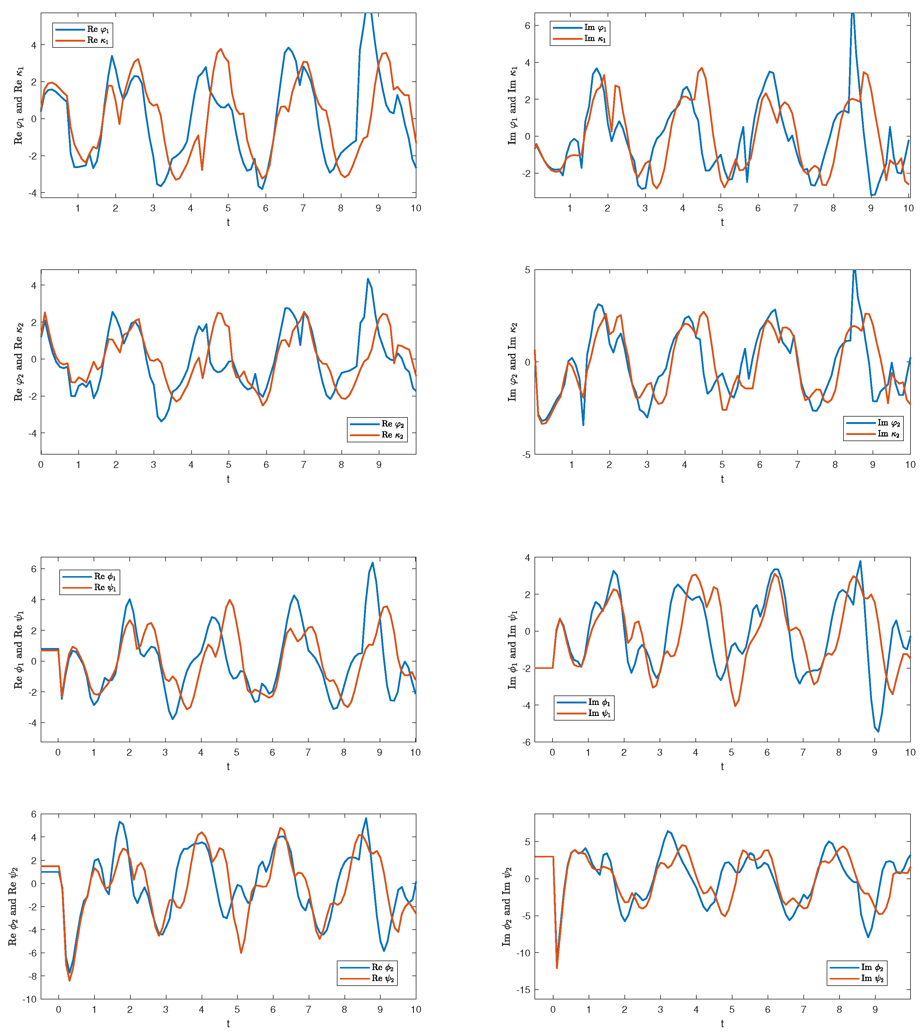
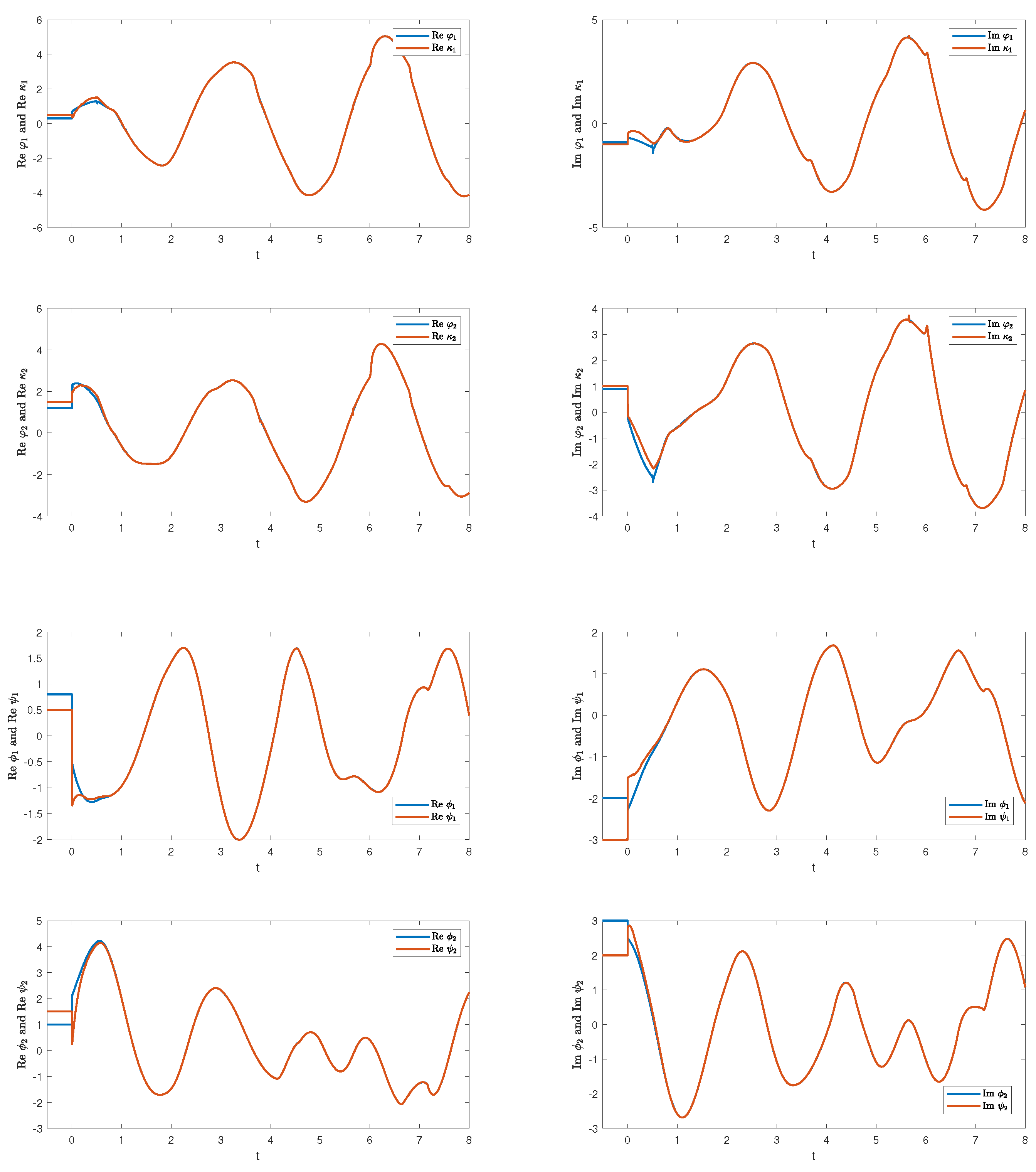
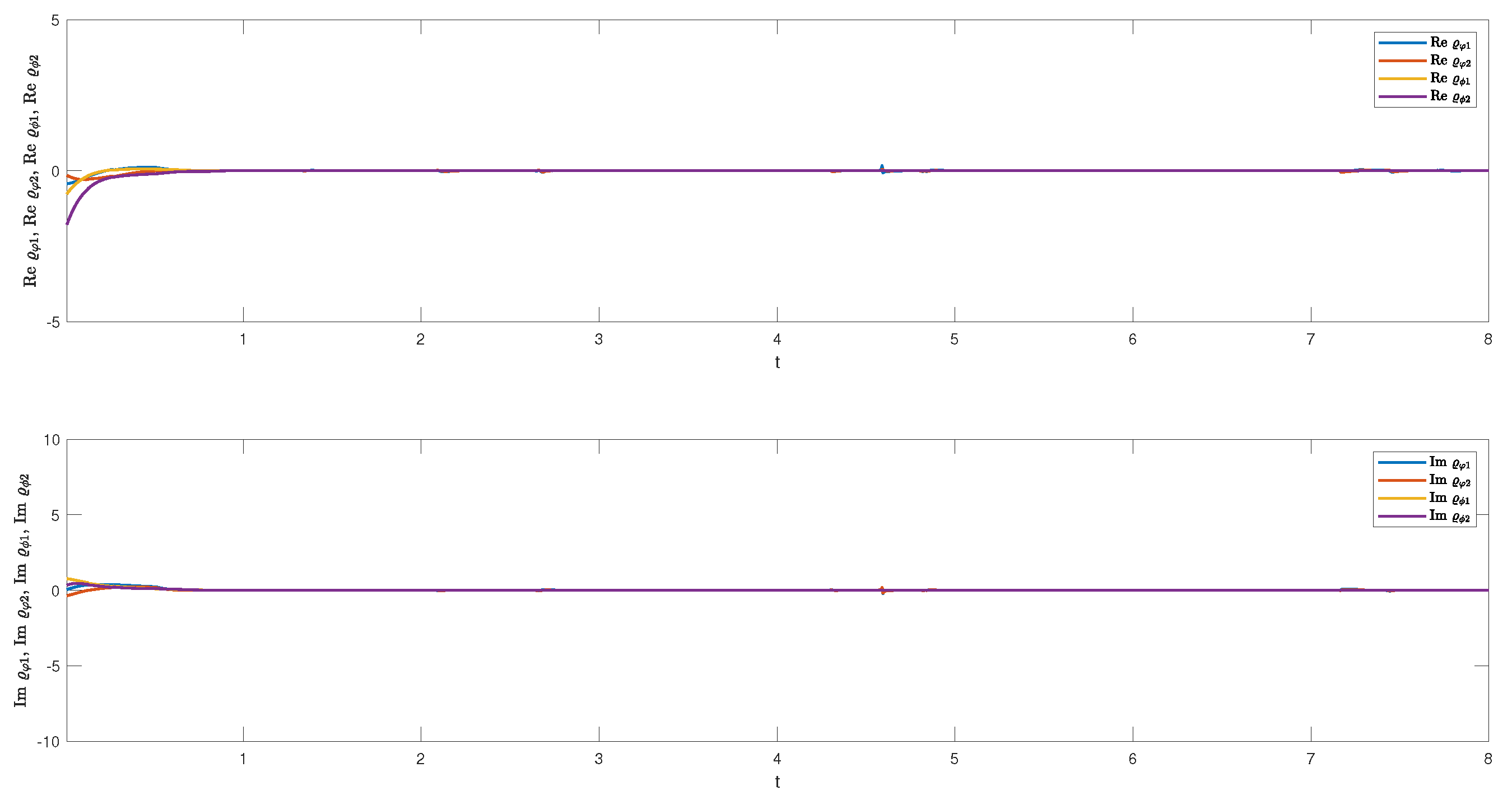
6. Numerical Examples

In this section, with the selection of values that match Assumptions 3 and 4, a numerical example is given to prove the effectiveness of proposed schemes.

Example 1.

Considering that the model is formed by the interaction of various small molecules, the following gene regulatory network with two dimensions is built as the drive system:

$$\left\{\begin{array}{cc}\hfill {}_0^C{D}_t^{\alpha }{\phi }_i\left(t\right)& =-a_i{\phi }_i\left(t\right)+\sum _{j=1}^n{\omega }_{ij}{\zeta }_j\left({\varphi }_j(t-{\tau }_1)\right)+B_i,\hfill \\ \hfill {}_0^C{D}_t^{\alpha }{\varphi }_i\left(t\right)& =-c_i{\varphi }_i\left(t\right)+d_i{\phi }_i(t-{\tau }_2),t⩾0,\hfill \end{array}\right.$$

(40)

where $i=1,2$, $\alpha =0.92$, ${\tau }_1={\tau }_2=0.5$${\zeta }_j\left({\varphi }_j(t-\tau )\right)={\displaystyle \frac{{\varphi }_j^2(t-\tau )}{{\varphi }_j^2(t-\tau )+1}}$, $j=1,2$, and $B_1=B_2=0$. Let the initial values of the model (40) be ${\phi }_1\left(t\right)=e^{0.3t-i0.9t}$, ${\phi }_2\left(t\right)=e^{1.2t+i0.9t}$, ${\varphi }_1\left(t\right)=e^{0.8t-i2t}$, ${\varphi }_2\left(t\right)=e^{1t+i3t}$, $t\in [-0.5,0]$, and

$$A=\left(\begin{array}{cc}1.2+4i& 0\\ 0& 1.4+4i\end{array}\right),W={\left({\omega }_{ij}\right)}_{2\times 2}=\left(\begin{array}{cc}2.3-0.3i& 3.5+0.6i\\ 2.8-0.5i& 1.5+0.4i\end{array}\right),$$

$$C=\left(\begin{array}{cc}2+5i& 0\\ 0& 3+5i\end{array}\right),D=\left(\begin{array}{cc}3+1i& 0\\ 0& 2-1i\end{array}\right).$$

The response system is

$$\left\{\begin{array}{cc}\hfill {}_0^C{D}_t^{\alpha }{\kappa }_i\left(t\right)& =-a_i{\kappa }_i\left(t\right)+\sum _{j=1}^n{\omega }_{ij}{\zeta }_j\left({\psi }_j(t-{\tau }_1)\right)+B_i+u_i\left(t\right),\hfill \\ \hfill {}_0^C{D}_t^{\alpha }{\psi }_i\left(t\right)& =-c_i{\psi }_i\left(t\right)+d_i{\kappa }_i(t-{\tau }_2)+\widetilde{u_i}\left(t\right),t⩾0,\hfill \end{array}\right.$$

(41)

where the initial values are ${\kappa }_1\left(t\right)=e^{0.4-1i}$, ${\kappa }_2\left(t\right)=e^{1.3+2i}$, ${\psi }_1\left(t\right)=e^{0.7-2i}$, and ${\psi }_2\left(t\right)=e^{1.5+3i}$, $t\in [-0.5,0]$.

First, as shown in Figure 1, it is clear that systems (40) and (41) cannot be synchronized without controllers.

Now, we will verify the synchronization between (40) and (41) by our proposed control schemes (9) and (23).

6.1. Synchronization by State Feedback Controller (9)

In the controller (9), let $k_1=k_2=10-5i$, ${\tilde{k}}_1={\tilde{k}}_2=4-i$, and $\eta =\tilde{\eta }=0.01+0.5i$. Then, we have

$$a_1+\overline{a_1}+k_1+\overline{k_1}-\sum _{j=1}^n|{\omega }_{1j}{|}_2^2=7.93\ge 0,c_1+\overline{c_1}+\widetilde{k_1}+\overline{\widetilde{k_1}}-l_1^2-{\left|d_1\right|}_2^2=2\ge 0,$$

$$a_2+\overline{a_2}+k_2+\overline{k_2}-\sum _{j=1}^n|{\omega }_{2j}{|}_2^2=6.78\ge 0,c_1+\overline{c_2}+\widetilde{k_2}+\overline{\widetilde{k_2}}-l_2^2-{\left|d_2\right|}_2^2=7\ge 0.$$

Thus, all assumptions and conditions in Theorem 1 hold, and it is easy to calculate that the setting time is estimated as $T=58.3433$. Thereupon, according to Theorem 1, (40) and (41) can achieve synchronization in finite time by controller (9). Figure 2 presents the state trajectories of drive system (40) and response system (41), and Figure 3 depicts the state trajectory of the error system between (40) and (41).

6.2. Synchronization by Adaptive Controller (23)

In the controller (23), let ${\theta }_1={\theta }_2=0.03+0.8i$, $\widetilde{{\theta }_1}=\widetilde{{\theta }_2}=0.02-0.7i$, ${\delta }_1={\delta }_2=0.4+i$, $\widetilde{{\delta }_1}=\widetilde{{\delta }_2}=7+3i$, $q_1=q_2=9+3i$, and $g_1=g_2=2+4i$. Similarly, according to the conditions of Theorem 2, in the controller (23), the synchronization of the drive-response system in finite time is shown in Figure 4, with an estimated time of $T=6.7739$, and the trajectory of the synchronization error system is shown in Figure 5.

7. Conclusions

This paper has investigated the problem of synchronization in finite time for fractional-order complex-valued gene regulatory networks with delays. Two different controllers have been designed to address this problem and a complex-valued sign function has been employed to solve this problem directly in a complex field instead of separating the system into two real-valued systems. Then, several appropriate criteria ensuring synchronization in finite time based on the designed controllers by using suitable Lyapunov functions and the stability theory of fractional systems have been presented. Additionally, the effectiveness of these theoretical results has been illustrated through a numerical example, and the simulation results have demonstrated that the instant of complete synchronization for the considered models based on the proposed adaptive controller is shorter than that based on the feedback controller.

References

1. De Jong, H. Modeling and simulation of genetic regulatory systems: A literature review. J. Comput. Biol. 2002, 9, 67–103. [Google Scholar] [CrossRef]
2. Casey, R.; Jong, H.; Gouzé, J.L. Piecewise-linear models of genetic regulatory networks: Equilibria and their stability. J. Math. Biol. 2006, 52, 27–56. [Google Scholar] [CrossRef]
3. Cao, Z.; Grima, R. Linear mapping approximation of gene regulatory networks with stochastic dynamics. Nat. Commun. 2018, 9, 1–15. [Google Scholar] [CrossRef]
4. Liu, F.; Zhang, S.W.; Guo, W.F.; Wei, Z.G.; Chen, L. Inference of gene regulatory network based on local Bayesian networks. PLoS Comput. Biol. 2016, 12, e1005024. [Google Scholar] [CrossRef]
5. Sanchez-Castillo, M.; Blanco, D.; Tienda-Luna, I.M.; Carrion, M.C.; Huang, Y. A Bayesian framework for the inference of gene regulatory networks from time and pseudo-time series data. Bioinformatics 2018, 34, 964–970. [Google Scholar] [CrossRef]
6. Tang, W.W.; Dietmann, S.; Irie, N.; Leitch, H.G.; Floros, V.I.; Bradshaw, C.R.; Surani, M.A. A unique gene regulatory network resets the human germline epigenome for development. Cell 2015, 161, 1453–1467. [Google Scholar] [CrossRef]
7. Zhang, X.; Wu, L.; Zou, J. Globally asymptotic stability analysis for genetic regulatory networks with mixed delays: An M-matrix-based approach. IEEE/ACM Trans. Comput. Biol. Bioinform. 2015, 13, 135–147. [Google Scholar] [CrossRef] [PubMed]
8. Liu, Z.P.; Wu, C.; Miao, H.; Wu, H. RegNetwork: An integrated database of transcriptional and post-transcriptional regulatory networks in human and mouse. Database 2015, 2015, bav095. [Google Scholar] [CrossRef] [PubMed]
9. Shmulevich, I.; Dougherty, E.R.; Kim, S.; Zhang, W. Probabilistic Boolean networks: A rule-based uncertainty model for gene regulatory networks. Bioinformatics 2002, 18, 261–274. [Google Scholar] [CrossRef] [PubMed]
10. Karlebach, G.; Shamir, R. Modelling and analysis of gene regulatory networks. Nat. Rev. Mol. Cell Biol. 2008, 9, 770–780. [Google Scholar] [CrossRef]
11. Rao, X.; Chen, X.; Shen, H.; Ma, Q.; Li, G.; Tang, Y.; Dixon, R.A. Gene regulatory networks for lignin biosynthesis in switchgrass (Panicum virgatum). Plant Biotechnol. J. 2019, 17, 580–593. [Google Scholar] [CrossRef] [PubMed]
12. Liu, W.; Jiang, Y.; Peng, L.; Sun, X.; Gan, W.; Zhao, Q.; Tang, H. Inferring gene regulatory networks using the improved Markov blanket discovery algorithm. Interdiscip. Sci. Comput. Life Sci. 2022, 14, 168–181. [Google Scholar] [CrossRef]
13. Pu, M.; Chen, J.; Tao, Z.; Miao, L.; Qi, X.; Wang, Y.; Ren, J. Regulatory network of miRNA on its target: Coordination between transcriptional and post-transcriptional regulation of gene expression. Cell. Mol. Life Sci. 2019, 76, 441–451. [Google Scholar] [CrossRef] [PubMed]
14. Zhang, Z.; Zhang, J.; Ai, Z. A novel stability criterion of the time-lag fractional-order gene regulatory network system for stability analysis. Commun. Nonlinear Sci. Numer. Simul. 2019, 66, 96–108. [Google Scholar] [CrossRef]
15. Leine, R.I.; Nijmeijer, H. Dynamics and Bifurcations of Non-Smooth Mechanical Systems; Springer Science & Business Media: Berlin/Heidelberg, Germany, 2013. [Google Scholar]
16. Van de Sande, B.; Flerin, C.; Davie, K.; De Waegeneer, M.; Hulselmans, G.; Aibar, S.; Aerts, S. A scalable SCENIC workflow for single-cell gene regulatory network analysis. Nat. Protoc. 2020, 15, 2247–2276. [Google Scholar] [CrossRef] [PubMed]
17. Pandiselvi, S.; Raja, R.; Cao, J.; Li, X.; Rajchakit, G. Impulsive discrete-time GRNs with probabilistic time delays, distributed and leakage delays: An asymptotic stability issue. Ima J. Math. Control. Inf. 2019, 36, 79–100. [Google Scholar] [CrossRef]
18. Senthilraj, S.; Raja, R.; Zhu, Q.; Samidurai, R.; Zhou, H. Delay-dependent asymptotic stability criteria for genetic regulatory networks with impulsive perturbations. Neurocomputing 2016, 214, 981–990. [Google Scholar] [CrossRef]
19. Zang, H.; Zhang, T.; Zhang, Y. Bifurcation analysis of a mathematical model for genetic regulatory network with time delays. Appl. Math. Comput. 2015, 260, 204–226. [Google Scholar] [CrossRef]
20. Lei, J.; Shatat, A.S.; Lakys, Y. Fractional Differential Equations in Electronic Information Models. Appl. Math. Nonlinear Sci. 2022, 1–9. [Google Scholar]
21. Zhang, D.; Yang, L.; Arbab, A. The Uniqueness of Solutions of Fractional Differential Equations in University Mathematics Teaching Based on the Principle of Compression Mapping. Appl. Math. Nonlinear Sci. 2022, 1–7. [Google Scholar]
22. Ding, J. Abnormal Behavior of Fractional Differential Equations in Processing Computer Big Data. Appl. Math. Nonlinear Sci. 2022, 1–9. [Google Scholar] [CrossRef]
23. Kilbas, A.A.; Srivastava, H.M.; Trujillo, J.J. Theory and Applications of Fractional Differential Equations; Elsevier: Amsterdam, The Netherlands, 2006. [Google Scholar]
24. Zhang, Y.; Pu, Y.; Zhang, H.; Cong, Y.; Zhou, J. An extended fractional Kalman filter for inferring gene regulatory networks using time-series data. Chemom. Intell. Lab. Syst. 2014, 138, 57–63. [Google Scholar] [CrossRef]
25. Wang, L.; Song, Q.; Liu, Y.; Zhao, Z.; Alsaadi, F.E. Finite-time stability analysis of fractional-order complex-valued memristor-based neural networks with both leakage and time-varying delays. Neurocomputing 2017, 245, 86–101. [Google Scholar] [CrossRef]
26. Zhang, P.; Wu, W.; Chen, Q.; Chen, M. Non-coding RNAs and their integrated networks. J. Integr. Bioinform. 2019, 16, 20190027. [Google Scholar] [CrossRef]
27. Wan, X.; Wang, Z.; Wu, M.; Liu, X. State estimation for discrete time-delayed genetic regulatory networks with stochastic noises under the round-robin protocols. IEEE Trans. Nanobiosci. 2018, 17, 145–154. [Google Scholar] [CrossRef] [PubMed]
28. Luo, Y.; Chen, Y. Fractional order [proportional derivative] controller for a class of fractional order systems. Automatica 2009, 45, 2446–2450. [Google Scholar] [CrossRef]
29. Zhang, Z.; Wang, Y.; Zhang, J.; Cheng, F.; Liu, F.; Ding, C. Novel asymptotic stability criterion for fractional-order gene regulation system with time delay. Asian J. Control 2022, 24, 3095–3104. [Google Scholar] [CrossRef]
30. Huang, C.; Cao, J.; Xiao, M.; Alsaedi, A.; Hayat, T. Bifurcations in a delayed fractional complex-valued neural network. Appl. Math. Comput. 2017, 292, 210–227. [Google Scholar] [CrossRef]
31. Zheng, Y.G.; Wang, Z.H. Stability and Hopf bifurcation of a class of TCP/AQM networks. Nonlinear Anal. Real World Appl. 2010, 11, 1552–1559. [Google Scholar] [CrossRef]
32. Guan, Z.H.; Yue, D.; Hu, B.; Li, T.; Liu, F. Cluster synchronization of coupled genetic regulatory networks with delays via aperiodically adaptive intermittent control. IEEE Trans. Nanobiosci. 2017, 16, 585–599. [Google Scholar] [CrossRef]
33. Zou, Y.; Su, H.; Tang, R.; Yang, X. Finite-time bipartite synchronization of switched competitive neural networks with time delay via quantized control. ISA Trans. 2022, 125, 156–165. [Google Scholar] [CrossRef]
34. Xujun, Y.; Qiankun, S.; Yurong, L.; Zhenjiang, Z. Finite-time stability analysis of fractional-order neural networks with delay. Neurocomputing 2015, 152, 19–26. [Google Scholar]
35. Li, M.; Yang, X.; Song, Q.; Chen, X. Robust Asymptotic Stability and Projective Synchronization of Time-Varying Delayed Fractional Neural Networks Under Parametric Uncertainty. Neural Process. Lett. 2022, 54, 4661–4680. [Google Scholar] [CrossRef]
36. Du, F.; Lu, J.G. New criterion for finite-time synchronization of fractional order memristor-based neural networks with time delay. Appl. Math. Comput. 2021, 389, 125616. [Google Scholar] [CrossRef]
37. Rakkiyappan, R.; Cao, J.; Velmurugan, G. Existence and uniform stability analysis of fractional-order complex-valued neural networks with time delays. IEEE Trans. Neural Netw. Learn. Syst. 2014, 26, 84–97. [Google Scholar] [CrossRef] [PubMed]
38. Udhayakumar, K.; Rakkiyappan, R.; Rihan, F.A.; Banerjee, S. Projective multi-synchronization of fractional-order complex-valued coupled multi-stable neural networks with impulsive control. Neurocomputing 2022, 467, 392–405. [Google Scholar] [CrossRef]
39. Wu, Z.; Wang, Z.; Zhou, T. Global stability analysis of fractional-order gene regulatory networks with time delay. Int. J. Biomath. 2019, 12, 1950067. [Google Scholar] [CrossRef]
40. Syed Ali, M.; Narayanan, G.; Orman, Z.; Shekher, V.; Arik, S. Finite time stability analysis of fractional-order complex-valued memristive neural networks with proportional delays. Neural Process. Lett. 2020, 51, 407–426. [Google Scholar] [CrossRef]
41. Zheng, B.; Hu, C.; Yu, J.; Jiang, H. Finite-time synchronization of fully complex-valued neural networks with fractional-order. Neurocomputing 2020, 373, 70–80. [Google Scholar] [CrossRef]
42. Zeng, J.; Yang, X.; Wang, L.; Chen, X. Robust Asymptotical Stability and Stabilization of Fractional-Order Complex-Valued Neural Networks with Delay. Discret. Dyn. Nat. Soc. 2021, 2021, 5653791. [Google Scholar] [CrossRef]
43. Chen, J.; Chen, B.; Zeng, Z. Global asymptotic stability and adaptive ultimate Mittag–Leffler synchronization for a fractional-order complex-valued memristive neural networks with delays. IEEE Trans. Syst. Man Cybern. Syst. 2018, 49, 2519–2535. [Google Scholar] [CrossRef]
44. Xu, Y.; Li, Y.; Li, W. Adaptive finite-time synchronization control for fractional-order complex-valued dynamical networks with multiple weights. Commun. Nonlinear Sci. Numer. Simul. 2020, 85, 105239. [Google Scholar] [CrossRef]
45. Pecora, L.M.; Carroll, T.L. Synchronization in chaotic systems. Phys. Rev. Lett. 1990, 64, 821. [Google Scholar] [CrossRef]
46. Jiang, N.; Liu, X.; Yu, W.; Shen, J. Finite-time stochastic synchronization of genetic regulatory networks. Neurocomputing 2015, 167, 314–321. [Google Scholar] [CrossRef]
47. Liu, F.; Zhang, Z.; Wang, X.; Sun, F. Stability and synchronization control of fractional-order gene regulatory network system with delay. J. Adv. Comput. Intell. Intell. Inform. 2017, 21, 148–152. [Google Scholar] [CrossRef]
48. Qiao, Y.; Yan, H.; Duan, L.; Miao, J. Finite-time synchronization of fractional-order gene regulatory networks with time delay. Neural Netw. 2020, 126, 1–10. [Google Scholar] [CrossRef]
49. Podlubny, I. Fractional Differential Equations: An Introduction to Fractional Derivatives; Academic Press: New York, NY, USA, 1998. [Google Scholar]
50. Yang, S.; Yu, J.; Hu, C.; Jiang, H. Quasi-projective synchronization of fractional-order complex-valued recurrent neural networks. Neural Netw. 2018, 104, 104–113. [Google Scholar] [CrossRef]
51. Yu, J.; Hu, C.; Jiang, H. Corrigendum to Projective synchronization for fractional neural networks. Neural Netw. 2015, 67, 152–154. [Google Scholar] [CrossRef]
52. Li, Y.; Yang, X.; Shi, L. Finite-time synchronization for competitive neural networks with mixed delays and non-identical perturbations. Neurocomputing 2016, 185, 242–253. [Google Scholar] [CrossRef]
53. Baleanu, D.; Sadati, S.J.; Ghaderi, R.; Ranjbar, A.; Jarad, F. Razumikhin stability theorem for fractional systems with delay. Abstr. Appl. Anal. 2010, 2010, 124812. [Google Scholar] [CrossRef]
Figure 1. State trajectories of (40) and (41) without controller.
Fractalfract 07 00347 g001
Figure 2. State trajectories of (40) and (41) under controller (9).
Fractalfract 07 00347 g002
Figure 3. State trajectories of error system under controller (9).
Fractalfract 07 00347 g003
Figure 4. State trajectories of (40) and (41) under controller (23).
Fractalfract 07 00347 g004
Figure 5. The synchronization trajectories of error system under controller (23).
Fractalfract 07 00347 g005
Disclaimer/Publisher’s Note: The statements, opinions and data contained in all publications are solely those of the individual author(s) and contributor(s) and not of MDPI and/or the editor(s). MDPI and/or the editor(s) disclaim responsibility for any injury to people or property resulting from any ideas, methods, instructions or products referred to in the content.