Article

Enhancing the Mathematical Theory of Nabla Tempered Fractional Calculus: Several Useful Equations

1
School of Mathematics, Southeast University, Nanjing 211189, China
2
School of Business, Nanjing Audit University, Nanjing 211815, China
3
Yonsei Frontier Lab, Yonsei University, Seoul 03722, Republic of Korea
*
Author to whom correspondence should be addressed.
Fractal Fract. 2023, 7(4), 330; https://doi.org/10.3390/fractalfract7040330
Submission received: 20 March 2023 / Revised: 9 April 2023 / Accepted: 11 April 2023 / Published: 14 April 2023
(This article belongs to the Special Issue Advances in Fractional-Order Neural Networks, Volume II)

Abstract

:
Although many applications of fractional calculus have been reported in literature, modeling the physical world using this technique is still a challenge. One of the main difficulties in solving this problem is that the long memory property is necessary, whereas the infinite memory is undesirable. To address this challenge, a new type of nabla fractional calculus with a weight function is formulated, which combines the benefits of nabla fractional calculus and its tempered counterpart, making it highly valuable for modeling practical systems. However, many properties of this calculus are still unclear and need to be discovered. Therefore, this paper gives particular emphasis to the topic, developing some remarkable properties, i.e., the equivalence relation, the nabla Taylor formula, and the nabla Laplace transform of such nabla tempered fractional calculus. All the developed properties greatly enrich the mathematical theory of nabla tempered fractional calculus and provide high value and potential for further applications.

1. Introduction

Fractional calculus has become an important tool in various fields of science and engineering due to its ability to describe and analyze complex systems with the long memory property [1,2,3]. However, the long memory property of fractional calculus also poses many challenges in modeling some special objects because the length of memory is increasing and unbounded as time goes on. To overcome these difficulties, the concept of tempered fractional calculus has been introduced in recent decades [4,5]. Tempered fractional calculus involves an extra weight function, which allows for the control of the memory length. With special selection of weight function, this has led to new insights, inspirations, and developments in the field of fractional calculus, as it provides a way to accurately model complex systems with adjustable memory. These advantages have motivated many researchers to explore the subject of tempered fractional calculus, leading to significant progress in the field in recent years [6,7,8]. Tempered fractional calculus has become a hot topic in fractional order fields. Its potential applications are vast and expected to continue growing in the future.
Fernandez et al. performed some detailed analysis of the mathematical underpinnings of tempered fractional calculus. For example, they demonstrated some special functions that have an intrinsic connection to tempered fractional calculus and derived the related Taylor’s theorem, integral inequalities [9]. In a recent work [10], Fernandez et al. considered an increasing weight function, promoted the conjugation relations, and developed the Laplace transform. In addition, the tempered fractional calculus with respect to function was discussed preliminarily. Reference [11] concerned the tempered fractional calculus with respect to function, dealt with some analytical properties of such calculus, and also developed some properties for such fractional differential equations involving existence, uniqueness, data dependency, and stability. Gu et al. proposed a class of tempered fractional neural networks and developed the stability conditions involving the attractivity and the Mittag–Leffler stability [12]. Ortigueira et al. made a brief of substantial, tempered, shifted fractional derivatives and explored the relationship between these derivatives in a unified framework [13]. The numerical computation problem of tempered fractional differential equation was discussed in [14,15,16].
Compared with the continuous time tempered fractional calculus, the research in the discrete time case is just in its infancy and only a few studies has been reported. Abdeljawada et al. introduced definitions of delta tempered fractional calculus, investigated its memory effect, and applied it to image processing [17]. Fu et al. extended the time scale Z to h Z , defined both the delta/nabla tempered fractional calculus, and derived the solution of a nonlinear system [18]. Ferreira generalized the exponential weight function to the nonzero case and discussed its application in entropy analysis [19]. With the developed nabla tempered fractional calculus, the authors defined the tempered Mittag–Leffler stability and derived the fractional difference inequality, the comparison principle, and the Lyapunov criteria [20]. Due to the existence of weight functions in tempered fractional calculus, such calculus has some essential characteristics different from the classical fractional counterpart, which are far from clarifying.
Although the study on discrete time tempered fractional calculus is still insufficient, a proliferation of results reported on discrete time fractional calculus [21,22,23,24,25] could give us much helpful inspiration. The basic arithmetic and equivalence relations of fractional difference and fractional sum were discussed in [21,22,23]. The continuity on the order of fractional difference was studied in [21,23,26]. However, the Grünwald–Letnikov difference is not equivalent to the classical integer order case when the order is assumed to be an integer, which means that the existing results need extra conditions. The nabla Taylor series was first investigated systematically in [26], although some of the existing results require quite strict conditions and the nabla Taylor formula expanded at the current time was not discussed enough. A brief review was made on the nabla Laplace transform [27], and some interesting properties still could be built with the existing results. Bearing these in mind, the primary objective of this study is to establish some analytical properties of nabla tempered fractional calculus. In particular, some similar properties, such as the semigroup property and the limit property, will be checked under three well-known definitions. The nabla Taylor series, the nabla Taylor formula, and the Leibniz rule will be built for nabla tempered fractional calculus. The Laplace transform and its application on difference transfer property will be discussed for the suggested calculus. However, it is not easy to complete this task, as the introduction of the weight function brings some unexpected difficulty and damages some accustomed properties.
The remainder of this paper is summarized as follows. In Section 2, the basic concept and properties of nabla tempered fractional calculus are presented. In Section 3, many foundational properties are developed for such fractional calculus. In Section 4, a simulation study is performed to illustrate the validity of the developed results. In Section 5, some concluding remarks are provided to end this paper.

2. Preliminaries

In this section, the definitions and properties for nabla tempered fractional calculus are introduced.
Definition 1.
([22] Definition 2.1) For x : N a + 1 n R , its nth nabla difference is defined by
n x ( k ) : = i = 0 n ( 1 ) i n i x ( k i ) ,
where n Z + , k N a + 1 : = { a + 1 , a + 2 , } , a R , p q : = Γ ( p + 1 ) Γ ( q + 1 ) Γ ( p q + 1 ) is the generalized binomial coefficient and Γ ( · ) is the Gamma function.
Definition 2.
([22] Definition 3.1) For x : N a + 1 R , its αth Grünwald–Letnikov difference/sum is defined by
a G k α x ( k ) : = i = 0 k a 1 ( 1 ) i α i x ( k i ) ,
where α R , k N a + 1 and a R .
When α > 0 , a G k α x ( k ) represents the difference operation. When α < 0 , a G k α x ( k ) represents the sum operation including the fractional order case and the integer order case. Specially, a G k 0 x ( k ) = x ( k ) . Even though α = n Z + , a G k α x ( k ) n x ( k ) for all k N a + 1 .
Defining the rising function p q ¯ : = Γ ( p + q ) Γ ( p ) , p Z + , q R , by applying Γ ( θ ) Γ ( 1 θ ) = π sin ( π θ ) , θ R and replace the summing order, it follows that
a G k α x ( k ) = i = 0 k a 1 ( 1 ) i Γ ( 1 + α ) Γ ( i + 1 ) Γ ( 1 + α i ) x ( k i ) = i = 0 k a 1 Γ ( i α ) Γ ( i + 1 ) Γ ( α ) x ( k i ) = i = 0 k a 1 ( i + 1 ) α 1 ¯ Γ ( α ) x ( k i ) = i = a + 1 k ( k i + 1 ) α 1 ¯ Γ ( α ) x ( i ) ,
which will play a key role in subsequent analysis.
Definition 3.
([22] Definitions 3.4 and 3.5) For x : N a + 1 n R , its αth Riemann–Liouville fractional difference and Caputo fractional difference are defined by
a R k α x ( k ) : = n a G k α n x ( k ) ,
a C k α x ( k ) : = a G k α n n x ( k ) ,
respectively, where α ( n 1 , n ) , n Z + , k N a + 1 and a R .
On this basis, the following properties hold.
Lemma 1.
[23,28] For any x : N a + 1 n R , α ( n 1 , n ) , k N a + 1 , n Z + , a R , one has
a R k α a G k α x ( k ) = a C k α a G k α x ( k ) = x ( k ) ,
a G k α a R k α x ( k ) = x ( k ) i = 0 n 1 ( k a ) α i 1 ¯ Γ ( α i ) [ a R k α i 1 x ( k ) ] k = a ,
a G k α a C k α x ( k ) = x ( k ) i = 0 n 1 ( k a ) i ¯ i ! [ i x ( k ) ] k = a .
With the well defined fractional difference and fractional sum, the concept of nabla fractional calculus can be developed by introducing the weight function w : N a + 1 R { 0 } .
Definition 4.
([19] Definition 2.4) For x : N a + 1 R , its αth Grünwald–Letnikov tempered difference/sum is defined by
a G k α , w ( k ) x ( k ) : = w 1 ( k ) a G k α [ w ( k ) x ( k ) ] ,
where α R , k N a + 1 , a R and w : N a + 1 R { 0 } .
Definition 5.
([19] Definition 2.9) The nth nabla tempered difference, the αth Riemann–Liouville tempered fractional difference, and Caputo tempered fractional difference of x : N a + 1 n R can be defined by
n , w ( k ) x ( k ) : = w 1 ( k ) n [ w ( k ) x ( k ) ] ,
a R k α , w ( k ) x ( k ) : = w 1 ( k ) a R k α [ w ( k ) x ( k ) ] ,
a C k α , w ( k ) x ( k ) : = w 1 ( k ) a C k α [ w ( k ) x ( k ) ] ,
respectively, where α ( n 1 , n ) , n Z + , k N a + 1 , a R and w : N a + 1 R { 0 } .
On this basis, the following relationships hold
a R k α , w ( k ) x ( k ) = n , w ( k ) a G k α n , w ( k ) x ( k ) ,
a C k α , w ( k ) x ( k ) = a G k α n , w ( k ) n , w ( k ) x ( k ) .
The equivalent condition of w : N a + 1 R { 0 } is finite nonzero. In this work, when w ( k ) = ( 1 λ ) k a , λ R { 1 } , the operations n , w ( k ) x ( k ) , a G k α , w ( k ) x ( k ) , a R k α , w ( k ) x ( k ) , a C k α , w ( k ) x ( k ) could be abbreviated as n , λ x ( k ) , a G k α , λ x ( k ) , a R k α , λ x ( k ) , a C k α , λ x ( k ) , respectively. Notably, this special case is still different from the one in [19], i.e., w ( k ) = ( 1 λ ) k . The adopted one facilitates the use and analysis. Compared to existing results, the tempered function w ( k ) is no longer limited to the exponential function, which makes this work more general and practical.
By using the linearity, the following lemmas can be derived immediately, which is simple while useful for understanding such fractional calculus. Therefore, the proof is omitted here.
Lemma 2.
For any x : N a + 1 n R , n Z + , a R , w : N a + 1 R { 0 } , α ( n 1 , n ) , k N a + 1 , ρ R { 0 } , one has
n , w ( k ) x ( k ) = n , ρ w ( k ) x ( k ) , a G k α , w ( k ) x ( k ) = a G k α , ρ w ( k ) x ( k ) , a G k α , w ( k ) x ( k ) = a G k α , ρ w ( k ) x ( k ) , a R k α , w ( k ) x ( k ) = a R k α , ρ w ( k ) x ( k ) , a C k α , w ( k ) x ( k ) = a C k α , ρ w ( k ) x ( k ) .
Note that Lemma 2 is indeed the scale invariance. When ρ = 1 , the sign of w ( k ) is just reversed to ρ w ( k ) . From this, one is ready to claim that if a property on tempered calculus holds for w ( k ) > 0 , it also holds for w ( k ) < 0 .
Lemma 3.
For any x : N a + 1 n R , n Z + , a R , α ( n 1 , n ) , β ( m 1 , m ) , m Z + , m n , w : N a + 1 R { 0 } , k N a + 1 , a R , one has
a R k n β , w ( k ) a C k β , w ( k ) x ( k ) = n , w ( k ) x ( k ) , a R k β , w ( k ) a C k n β , w ( k ) x ( k ) = n , w ( k ) x ( k ) , a C k n β , w ( k ) a R k β , w ( k ) x ( k ) = a G k n , w ( k ) x ( k ) , a C k β , w ( k ) a R k n β , w ( k ) x ( k ) = a G k n , w ( k ) x ( k ) .
Lemma 3 gives the semigroup properties for different tempered differences, which can be adopted to simplify the nabla tempered fractional difference equations.

3. Main Results

In this section, a series of nice properties will be nicely developed on the nabla tempered fractional calculus.

3.1. The Basic Relationship

In this part, the relationship between tempered nabla fractional difference/sum will be discussed.
Theorem 1.
For any x : N a + 1 n R , α ( n 1 , n ) , n Z + , k N a + 1 , a R , w : N a + 1 R { 0 } , one has
a R k α , w ( k ) x ( k ) = a G k α , w ( k ) x ( k ) ,
a R k α , w ( k ) x ( k ) = a C k α , w ( k ) x ( k ) + i = 0 n 1 ( k a ) i α ¯ Γ ( i α + 1 ) w ( a ) w ( k ) [ i , w ( k ) x ( k ) ] k = a ,
a G k α , w ( k ) x ( k ) = n , w ( k ) a G k α n , w ( k ) x ( k ) .
Proof of Theorem 1.
Taking first order difference with regard to k, one has ( k j + 1 ) β ¯ Γ ( β + 1 ) = ( k j + 1 ) β 1 ¯ Γ ( β ) , β R Z + and j = a + 1 k f ( j , k ) = j = a + 1 k f ( j , k ) + f ( k , k 1 ) , which coincides with [23] (Theorems 3.57 and 3.41). Letting z ( k ) : = w ( k ) x ( k ) and applying the aforementioned equations, one has
a R k α , w ( k ) x ( k ) = ( 11 ) w 1 ( k ) a R k α z ( k ) = ( 4 ) w 1 ( k ) n a G k α n z ( k ) = ( 3 ) w 1 ( k ) n j = a + 1 k ( k j + 1 ) n α 1 ¯ Γ ( n α ) z ( j ) = w 1 ( k ) n 1 [ j = a + 1 k ( k j + 1 ) n α 1 ¯ Γ ( n α ) z ( j ) + 0 n α 1 ¯ Γ ( n α ) z ( k ) ] = w 1 ( k ) n 1 j = a + 1 k ( k j + 1 ) n α 2 ¯ Γ ( n α 1 ) z ( j ) + w 1 ( k ) 0 n α 1 ¯ Γ ( n α ) n 1 z ( k ) = w 1 ( k ) n 2 j = a + 1 k ( k j + 1 ) n α 2 ¯ Γ ( n α 1 ) z ( j ) + w 1 ( k ) 0 n α 2 ¯ Γ ( n α 1 ) n 2 z ( k ) + w 1 ( k ) 0 n α 1 ¯ Γ ( n α ) n 1 z ( k ) = w 1 ( k ) j = a + 1 k ( k j + 1 ) α 1 ¯ Γ ( α ) z ( j ) + w 1 ( k ) i = 0 n 1 0 i α ¯ Γ ( i α + 1 ) i z ( k ) = ( 3 ) a G k α , w ( k ) x ( k ) + i = 0 n 1 0 i α ¯ Γ ( i α + 1 ) i , w ( k ) x ( k ) ,
which implies Equation (15) because of 0 β ¯ Γ ( 1 β ) = 0 , β R Z + and the finite i , w ( k ) x ( k ) , i = 0 , 1 , , n 1 , k N a + 1 .
Taking the first order difference with regard to j, one has ( k j ) β ¯ Γ ( β + 1 ) = ( k j + 1 ) β 1 ¯ Γ ( β ) , β R Z + . By applying the formula of summation by parts in [23] (Theorem 3.39), i.e., j = a + 1 k f ( j ) g ( j ) = [ f ( j ) g ( j ) ] j = a j = k j = a + 1 k f ( j 1 ) g ( j ) , it follows
a G k α , w ( k ) x ( k ) = ( 9 ) w 1 ( k ) a G k α z ( k ) = ( 3 ) w 1 ( k ) j = a + 1 k ( k j + 1 ) α 1 ¯ Γ ( α ) z ( j ) = w 1 ( k ) j = a + 1 k ( k j ) α ¯ Γ ( 1 α ) z ( j ) = w 1 ( k ) ( k a ) α ¯ Γ ( 1 α ) z ( a ) w 1 ( k ) 0 α ¯ Γ ( 1 α ) z ( k ) + w 1 ( k ) j = a + 1 k ( k j + 1 ) α ¯ Γ ( 1 α ) z ( j ) = w 1 ( k ) j = a + 1 k ( k j ) 1 α ¯ Γ ( 2 α ) z ( j ) + w 1 ( k ) ( k a ) α ¯ Γ ( 1 α ) z ( a ) w 1 ( k ) 0 α ¯ Γ ( 1 α ) z ( k ) = w 1 ( k ) j = a + 1 k ( k j + 1 ) n α 1 ¯ Γ ( n α + 1 ) n z ( j ) + w 1 ( k ) i = 0 n 1 ( k a ) i α ¯ Γ ( i α + 1 ) [ i z ( k ) ] k = a w 1 ( k ) i = 0 n 1 0 i α ¯ Γ ( i α + 1 ) i z ( k ) = ( 12 ) a C k α , w ( k ) x ( k ) + i = 0 n 1 ( k a ) i α ¯ Γ ( i α + 1 ) w ( a ) w ( k ) [ i , w ( k ) x ( k ) ] k = a i = 0 n 1 0 i α ¯ Γ ( i α + 1 ) i , w ( k ) x ( k ) .
The result in Equation (16) follows immediately by combining the above two equations.
Utilizing [28] (Theorem 4), one has
a G k α , w ( k ) x ( k ) = ( 9 ) w 1 ( k ) a G k α z ( k ) = w 1 ( k ) n a G k α n z ( k ) = w 1 ( k ) n w ( k ) w 1 ( k ) a G k α n w ( k ) x ( k ) = ( 10 ) n , w ( k ) a G k α n , w ( k ) x ( k ) ,
which is just (17). The proof is completed. □
Theorem 1 presents the basic relation between different fractional differences. Note that the finite value assumption on i , w ( k ) x ( k ) is not necessary for Equation (16). When w ( k ) = 1 , the tempered case in Theorem 1 reduces to the classical case ([28] Theorem 4, [26] Theorem 3). Equations (15) and (16) develop the relation between three well-known differences. Equation (17) implies that the tempered Grünwald–Letnikov sum can be described in the form of the tempered Riemann–Liouville difference. Notably, the condition of w ( k ) 0 is very common, and it can be positive or negative, for example, w ( k ) = sin k π a π + π 4 , k N a + 1 .
Theorem 2.
For any α ( n 1 , n ) , n Z + , w : N a + 1 R { 0 } , k N a + 1 , a R , one has
a G k α , w ( k ) a G k α , w ( k ) x ( k ) = a R k α , w ( k ) a G k α , w ( k ) x ( k ) = a C k α , w ( k ) a G k α , w ( k ) x ( k ) = x ( k ) ,
a G k α , w ( k ) a R k α , w ( k ) x ( k ) = x ( k ) i = 0 n 1 ( k a ) α i 1 ¯ Γ ( α i ) w ( a ) w ( k ) [ a R k α i 1 , w ( k ) x ( k ) ] k = a ,
a G k α , w ( k ) a C k α , w ( k ) x ( k ) = x ( k ) i = 0 n 1 ( k a ) i ¯ i ! w ( a ) w ( k ) [ i , w ( k ) x ( k ) ] k = a .
Proof of Theorem 2.
Using [28] (Corollary 1), one has
a G k α , w ( k ) a G k α , w ( k ) x ( k ) = w 1 ( k ) a G k α a G k α [ w ( k ) x ( k ) ] = w 1 ( k ) a G k 0 [ w ( k ) x ( k ) ] = w 1 ( k ) w ( k ) x ( k ) = x ( k ) .
From Lemma 1 and [28] (Theorem 2), one has
a R k α , w ( k ) a G k α , w ( k ) x ( k ) = n , w ( k ) a G k α n , w ( k ) a G k α , w ( k ) x ( k ) = w 1 ( k ) n a G k α n a G k α [ w ( k ) x ( k ) ] = w 1 ( k ) n a G k n [ w ( k ) x ( k ) ] = x ( k ) .
Similarly, by using Lemma 1 and [28] (Theorem 4), it follows that
a C k α , w ( k ) a G k α , w ( k ) x ( k ) = a G k α n , w ( k ) n , w ( k ) a G k α , w ( k ) x ( k ) = w 1 ( k ) a G k α n n a G k α [ w ( k ) x ( k ) ] = w 1 ( k ) a G k α n a G k n α [ w ( k ) x ( k ) ] = w 1 ( k ) a G k 0 [ w ( k ) x ( k ) ] = x ( k ) .
Combining the two mentioned equations yields Equation (18).
Assuming z ( k ) : = w ( k ) x ( k ) , considering the first order difference with regard to j, and using j = a + 1 k f ( j ) g ( j ) = [ f ( j ) g ( j ) ] j = a j = k j = a + 1 k f ( j 1 ) g ( j ) , it follows that
a G k α , w ( k ) a R k α , w ( k ) x ( k ) = w 1 ( k ) a G k α a R k α z ( k ) = w 1 ( k ) j = a + 1 k ( k j + 1 ) α 1 ¯ Γ ( α ) a R j α z ( j ) = w 1 ( k ) j = a + 1 k ( k j + 1 ) α 1 ¯ Γ ( α ) a R j α 1 z ( j ) = w 1 ( k ) [ ( k j ) α 1 ¯ Γ ( α ) a R j α 1 z ( j ) ] j = a j = k w 1 ( k ) j = a + 1 k ( k j ) α 1 ¯ Γ ( α ) a R j α 1 z ( j ) = w 1 ( k ) 0 α 1 ¯ Γ ( α ) a R k α 1 z ( k ) w 1 ( k ) ( k a ) α 1 ¯ Γ ( α ) [ a R k α 1 z ( k ) ] k = a + w 1 ( k ) j = a + 1 k ( k j + 1 ) α 2 ¯ Γ ( α 1 ) a R j α 2 z ( j ) = w 1 ( k ) i = 0 n 1 0 α i 1 ¯ Γ ( α i ) a R k α i 1 z ( k ) w 1 ( k ) i = 0 n 1 ( k a ) α i 1 ¯ Γ ( α i ) [ a R k α i 1 z ( k ) ] k = a + w 1 ( k ) j = a + 1 k ( k j + 1 ) α n 1 ¯ Γ ( α n ) a R j α n z ( j ) = i = 0 n 1 0 α i 1 ¯ Γ ( α i ) a R k α i 1 , w ( k ) x ( k ) i = 0 n 1 ( k a ) α i 1 ¯ Γ ( α i ) w ( a ) w ( k ) [ a R k α i 1 , w ( k ) x ( k ) ] k = a + w 1 ( k ) a G k n α a G k α n z ( k ) = w 1 ( k ) a G k 0 z ( k ) i = 0 n 1 ( k a ) α i 1 ¯ Γ ( α i ) w ( a ) w ( k ) [ a R k α i 1 , w ( k ) x ( k ) ] k = a ,
which implies Equation (19).
For the Caputo case, one has
a G k α , w ( k ) a C k α , w ( k ) x ( k ) = w 1 ( k ) a G k α a C k α z ( k ) = w 1 ( k ) a G k α a G k α n n z ( k ) = w 1 ( k ) a G k n n z ( k ) = w 1 ( k ) z ( k ) w 1 ( k ) i = 0 n 1 ( k a ) i ¯ i ! [ i z ( k ) ] k = a = ( 10 ) x ( k ) i = 0 n 1 w ( a ) w ( k ) ( k a ) i ¯ i ! [ i , w ( k ) x ( k ) ] k = a ,
which leads to Equation (20). All of these complete the proof. □
Theorem 2 gives the relation between tempered fractional difference and tempered fractional sum, which can be the generalization of [26] (Corollary 5). These properties can be adopted to derive the equivalent description of a nabla tempered fractional order system and calculate the solution.
By recalling Equation (20) and its derivation process, one has
x ( k ) = i = 0 n 1 ( k a ) i ¯ i ! w ( a ) w ( k ) [ i , w ( k ) x ( k ) ] k = a + j = a + 1 k ( k j + 1 ) α 1 ¯ Γ ( α ) w ( j ) w ( k ) a C j α , w ( j ) x ( j ) = i = 0 n 1 ( k a ) i ¯ i ! w ( a ) w ( k ) [ i , w ( k ) x ( k ) ] k = a + j = a + 1 k ( k j + 1 ) n 1 ¯ Γ ( n ) w ( j ) w ( k ) n , w ( j ) x ( j ) ,
which can be regarded as the nabla Taylor expansion of x ( k ) at k = a with summation reminder. The summation might be the fractional order case a G k α , w ( k ) a C k α , w ( k ) x ( k ) or the integer order case a G k n , w ( k ) n , w ( k ) x ( k ) .
In the same way, for any m Z + , m < α , one has
m , w ( k ) x ( k ) = i = m n 1 ( k a ) i m ¯ ( i m ) ! w ( a ) w ( k ) [ i , w ( k ) x ( k ) ] k = a + j = a + 1 k ( k j + 1 ) α m 1 ¯ Γ ( α m ) w ( j ) w ( k ) a C j α , w ( k ) x ( j ) .
From the definition, one can derive that
a G k n , w ( k ) x ( k ) = n , w ( k ) x ( k ) + i = k a n ( 1 ) i ( n i ) w ( k i ) w ( k ) x ( k i ) , k < a + n , 0 , k a + n ,
where n Z + , k N a + 1 , a R , and w ( k ) 0 . In other words, a G k n , w ( k ) x ( k ) is not always identical to n , w ( k ) x ( k ) . To explore more details, the limit of the fractional order case will be discussed.
Theorem 3.
For any x : N a + 1 R , α > 0 , k N a + 1 , a R , w : N a + 1 R { 0 } , a G k α , w ( k ) x ( k ) is continuous with respect to α and one has
lim α 0 a G k α , w ( k ) x ( k ) = x ( k ) .
Proof of Theorem 3.
By using Equations (6) and (9) and the formula of summation by parts, it follows that
a G k α , w ( k ) x ( k ) = w 1 ( k ) j = a + 1 k ( k j + 1 ) α 1 ¯ Γ ( α ) w ( j ) x ( j ) = w 1 ( k ) j = a + 1 k ( k j ) α ¯ Γ ( α + 1 ) w ( j ) x ( j ) = w 1 ( k ) j = a + 1 k ( k j + 1 ) α ¯ Γ ( α + 1 ) [ w ( j ) x ( j ) ] w 1 ( k ) ( k j ) α ¯ Γ ( α + 1 ) w ( j ) x ( j ) j = a j = k = w 1 ( k ) j = a + 1 k ( k j + 1 ) α ¯ Γ ( α + 1 ) [ w ( j ) x ( j ) ] + ( k a ) α ¯ Γ ( α + 1 ) w ( a ) w ( k ) x ( a ) .
Since ( k j + 1 ) α ¯ Γ ( α + 1 ) is continuous with respect to α for any j N a + 1 k , a G k α , w ( k ) x ( k ) is also continuous. Due to the fact of lim α 0 ( k j + 1 ) α ¯ Γ ( α + 1 ) = 1 , taking the limit for both sides of the above equation, one has
lim α 0 a G k α , w ( k ) x ( k ) = w 1 ( k ) j = a + 1 k [ w ( j ) x ( j ) ] + w ( a ) w ( k ) x ( a ) = x ( k ) .
The proof is thus done. □
In a similar way, the following corollary can be developed.
Corollary 1.
For any x : N a + 1 R , α ( 0 , 1 ) , k N a + 1 , a R , w : N a + 1 R { 0 } , a G k α , w ( k ) x ( k ) is continuous with respect to α and one has
lim α 0 a G k α , w ( k ) x ( k ) = x ( k ) .
Theorem 4.
For any x : N a + 1 n R , a R , n Z + , α ( n 1 , n ) , w : N a + 1 R { 0 } , a C k α , w ( k ) x ( k ) and a R k α , w ( k ) x ( k ) , k N a + 1 are continuous with respect to α, and the following limits hold:
lim α n a C k α , w ( k ) x ( k ) = n , w ( k ) x ( k ) ,
lim α n 1 a C k α , w ( k ) x ( k ) + w ( a ) w ( k ) [ n 1 , w ( k ) x ( k ) ] k = a = n 1 , w ( k ) x ( k ) ,
lim α n a R k α , w ( k ) x ( k ) = n , w ( k ) x ( k ) ,
lim α n 1 a R k α , w ( k ) x ( k ) = n 1 , w ( k ) x ( k ) .
Proof of Theorem 4.
Assume z ( k ) : = w ( k ) x ( k ) . The formula of summation by parts gives
a C k α , w ( k ) x ( k ) = w 1 ( k ) a C k α z ( k ) = w 1 ( k ) j = a + 1 k ( k j + 1 ) n α 1 ¯ Γ ( n α ) n z ( j ) = w 1 ( k ) j = a + 1 k ( k j ) n α ¯ Γ ( n α + 1 ) n z ( j ) = w 1 ( k ) j = a + 1 k ( k j + 1 ) n α ¯ Γ ( n α + 1 ) n + 1 z ( j ) + w 1 ( k ) ( k a ) n α ¯ Γ ( n α + 1 ) [ n z ( k ) ] k = a .
Note that ( k j + 1 ) n α 1 ¯ Γ ( n α ) is continuous regarding α for any j N a + 1 k k N a + 1 ; ( k a ) n α ¯ Γ ( n α + 1 ) is also continuous regarding α for any k N a + 1 . Therefore, a C k α , w ( k ) x ( k ) is also continuous. Due to the continuity of ( k a ) i α ¯ Γ ( i α + 1 ) with respect to α , i = 0 , 1 , , n 1 , k N a + 1 and the fact a R k α , w ( k ) x ( k ) = a C k α , w ( k ) x ( k ) + i = 0 n 1 ( k a ) i α ¯ Γ ( i α + 1 ) w ( a ) w ( k ) [ i , w ( k ) x ( k ) ] k = a , a R k α , w ( k ) x ( k ) is continuous with respect to α .
Taking the limit for α n and using Γ ( z ) = , z N , one has
lim α n a C k α , w ( k ) x ( k ) = lim α n w 1 ( k ) j = a + 1 k ( k j + 1 ) n α ¯ Γ ( n α + 1 ) n + 1 z ( j ) + lim α n w 1 ( k ) ( k a ) n α ¯ Γ ( n α + 1 ) [ n z ( k ) ] k = a = w 1 ( k ) j = a + 1 k lim α n ( k j + 1 ) n α ¯ Γ ( n α + 1 ) n + 1 z ( j ) + w 1 ( k ) lim α n ( k a ) n α ¯ Γ ( n α + 1 ) [ n z ( k ) ] k = a = w 1 ( k ) j = a + 1 k n + 1 z ( j ) + w 1 ( k ) [ n z ( k ) ] k = a = w 1 ( k ) n z ( k ) w 1 ( k ) [ n z ( k ) ] k = a + w 1 ( k ) [ n z ( k ) ] k = a = w 1 ( k ) n z ( k ) = n , w ( k ) x ( k ) .
For the case of α n 1 , it follows that
lim α n 1 a C k α , w ( k ) x ( k ) = lim α n 1 { w 1 ( k ) j = a + 1 k ( k j + 1 ) n α 1 ¯ Γ ( n α ) n z ( j ) } = w 1 ( k ) j = a + 1 k lim α n 1 ( k j + 1 ) n α 1 ¯ Γ ( n α ) n z ( j ) = w 1 ( k ) j = a + 1 k n z ( j ) = w 1 ( k ) n 1 z ( k ) w 1 ( k ) [ n 1 z ( k ) ] k = a = n 1 , w ( k ) x ( k ) w ( a ) w ( k ) [ n 1 , w ( k ) x ( k ) ] k = a ,
which smoothly leads to (23).
For any k N a + 1 , the following limit can be obtained:
lim α n i = 0 n 1 ( k a ) i α ¯ Γ ( i α + 1 ) w ( a ) w ( k ) [ i , w ( k ) x ( k ) ] k = a = i = 0 n 1 Γ ( k a + i n ) Γ ( i n + 1 ) Γ ( k a ) w ( a ) w ( k ) [ i , w ( k ) x ( k ) ] k = a = 0 .
On this basis, one has the following equation for k N a + 1 :
lim α n a R k α , w ( k ) x ( k ) = lim α n a C k α , w ( k ) x ( k ) + lim α n i = 0 n 1 ( k a ) i α ¯ Γ ( i α + 1 ) w ( a ) w ( k ) [ i , w ( k ) x ( k ) ] k = a = n , w ( k ) x ( k ) .
Similarly, for any k N a + 1 , it follows that
lim α n 1 a R k α , w ( k ) x ( k ) = lim α n 1 w 1 ( k ) j = a + 1 k ( k j + 1 ) n α 1 ¯ Γ ( n α ) n z ( j ) + lim α n 1 w 1 ( k ) i = 0 n 1 ( k a ) i α ¯ Γ ( i α + 1 ) [ i z ( k ) ] k = a = w 1 ( k ) j = a + 1 k n z ( j ) + w 1 ( k ) [ n 1 z ( k ) ] k = a = w 1 ( k ) n 1 z ( k ) = n 1 , w ( k ) x ( k ) .
Equation (24) is proved. □
Theorem 4 can be viewed as the generalization of [29] (page 781) and [23] (Theorem 3.63). Note that α ( n 1 , n ) , the adopted limit is the unilateral limit. When w ( k ) = 1 , Equations (23) and (24) reduce to the traditional nabla case in [23] (Theorem 3.63). Using Theorem 4, the range of α for a R k α , w ( k ) x ( k ) can be extended as [ n 1 , n ] , and the range of α for a C k α , w ( k ) x ( k ) should be ( n 1 , n ] .
Theorem 5.
For x , x i : N a + 1 b R , i Z + , if { x i } converges uniformly to x, then for any α > 0 , k , b N a + 1 , a R , w : N a + 1 R + or w : N a + 1 R , one has
lim i + a G k α , w ( k ) x i ( k ) = a G k α , w ( k ) x ( k ) .
Proof of Theorem 5.
Due to the given condition on uniform convergence, one obtains that for any ε > 0 , there exists N Z + , such that | x i ( k ) x ( k ) | < ε , for any i > N , k N a + 1 b . Assuming w : N a + 1 R + , κ : = max k a G k α , w ( k ) 1 and ϵ : = ε κ , then for any i > N , one has
| a G k α , w ( k ) x i ( k ) a G k α , w ( k ) x ( k ) | = | w 1 ( k ) j = a + 1 k ( k j + 1 ) α 1 ¯ Γ α w ( j ) [ x i ( j ) x ( j ) ] | w 1 ( k ) j = a + 1 k ( k j + 1 ) α 1 ¯ Γ α w ( j ) | x i ( j ) x ( j ) | ε w 1 ( k ) j = a + 1 k ( k j + 1 ) α 1 ¯ Γ α w ( j ) ε κ = ϵ ,
which implies Equation (25). By applying Lemma 2, it follows that Equation (25) still holds for w : N a + 1 R . □
Theorem 5 is inspired by [30] (Theorem 4), which can be used to find the limit of a G k α , w ( k ) x i ( k ) as i + and estimate the value of a G k α , w ( k ) x ( k ) . Different from the previous theorems, w ( k ) in Theorem 5 is assumed to be finite positive or finite negative.

3.2. Nabla Taylor Formula

In this part, some properties regarding the nabla Taylor formula and the nabla Taylor series of the nabla tempered fractional difference/sum will be developed. To this end, a useful lemma is given first.
Lemma 4.
([23] Theorem 3.48) For any x : N a K 1 R , a R , K N , k N a b , one has
x ( k ) = i = 0 K ( k a ) i ¯ i ! [ i x ( k ) ] k = a + j = a + 1 k ( k j + 1 ) K ¯ K ! K + 1 x ( j ) ,
which can be regarded as the nabla Taylor formula of x ( k ) expanded at the initial instant k = a .
Theorem 6.
For any x : N a K 1 R , a R , K N , n Z + , K > n , w : N a + 1 R { 0 } , k N a + 1 , one has
n , w ( k ) x ( k ) = i = n K ( k a ) i n ¯ ( i n ) ! w ( a ) w ( k ) [ i , w ( k ) x ( k ) ] k = a + j = a + 1 k ( k j + 1 ) K n ¯ Γ ( K n ) ! w ( j ) w ( k ) K + 1 , w ( j ) x ( j ) .
For any x : N a K 1 R , a R , K N , α R Z + , w : N a + 1 R { 0 } , k N a + 1 , one has
a G k α , w ( k ) x ( k ) = i = 0 K ( k a ) i α ¯ Γ ( i α + 1 ) w ( a ) w ( k ) [ i , w ( k ) x ( k ) ] k = a + j = a + 1 k ( k j + 1 ) K α ¯ Γ ( K α + 1 ) w ( j ) w ( k ) K + 1 , w ( j ) x ( j ) .
For any x : N a K 1 R , a R , K N , α ( n 1 , n ) , n Z + , w : N a + 1 R { 0 } , k N a + 1 , one has
a R k α , w ( k ) x ( k ) = i = 0 K ( k a ) i α ¯ Γ ( i α + 1 ) w ( a ) w ( k ) [ i , w ( k ) x ( k ) ] k = a + j = a + 1 k ( k j + 1 ) K α ¯ Γ ( K α + 1 ) w ( j ) w ( k ) K + 1 , w ( j ) x ( j ) .
For any x : N a K 1 R , a R , K N , α ( n 1 , n ) , n Z + , K > n , w : N a + 1 R { 0 } , k N a + 1 , one has
a C k α , w ( k ) x ( k ) = i = n K ( k a ) i α ¯ Γ ( i α + 1 ) w ( a ) w ( k ) [ i , w ( k ) x ( k ) ] k = a + j = a + 1 k ( k j + 1 ) K α ¯ Γ ( K α + 1 ) w ( j ) w ( k ) K + 1 , w ( j ) x ( j ) .
Proof of Theorem 6.
Letting z ( k ) : = w ( k ) x ( k ) , using Lemma 4, one has
z ( k ) = T K ( k ) + R K ( k ) ,
where T K ( k ) : = i = 0 K ( k a ) i ¯ i ! [ i z ( k ) ] k = a and R K ( k ) : = j = a + 1 k ( k j + 1 ) K ¯ K ! K + 1 z ( j ) =
a G k ( K + 1 ) K + 1 z ( k ) .
In the same way, j = a + 1 k f ( j ) g ( j ) = [ f ( j ) g ( j ) ] j = a j = k j = a + 1 k f ( j 1 ) g ( j ) leads to
n T K ( k ) = i = 0 K n k a i ¯ i ! [ i z k ] k = a = i = n K k a i n ¯ i n ! [ i z k ] k = a ,
n R K ( k ) = n 1 j = a + 1 k k j + 1 K ¯ K ! K + 1 z j = n 1 j = a + 1 k k j + 1 K ¯ K ! K + 1 z j + n 1 k j K ¯ K ! K + 1 z j j = k = n 1 j = a + 1 k k j + 1 K 1 ¯ ( K 1 ) ! K + 1 z j + 0 K ¯ K ! K + n z k = j = a + 1 k k j + 1 K n ¯ ( K n ) ! K + 1 z j + j = 1 n 0 K + n j ¯ ( K + n j ) ! K + j z k = j = a + 1 k k j + 1 K n ¯ ( K n ) ! K + 1 z j .
Using the above equations, one has
n , w ( k ) x ( k ) = w 1 ( k ) n z ( k ) = w 1 ( k ) n T K ( k ) + w 1 ( k ) n R K ( k ) = i = n K k a i n ¯ i n ! w ( a ) w ( k ) [ i , w ( k ) x k ] k = a + j = a + 1 k k j + 1 K n ¯ ( K n ) ! w ( j ) w ( k ) K + 1 , w ( j ) x j ,
which confirms Equation (27).
In a similar way, one has
a G k α , w ( k ) x ( k ) = w 1 ( k ) a G k α z ( k ) = w 1 ( k ) a G k α T K ( k ) + w 1 ( k ) a G k α R K ( k ) = w 1 ( k ) i = 0 K a G k α k a i ¯ i ! [ i z k ] k = a + w 1 ( k ) a G k α a G k ( K + 1 ) K + 1 z ( k ) = w 1 ( k ) i = 0 K k a i α ¯ Γ ( i α + 1 ) [ i z k ] k = a + w 1 ( k ) a G k α ( K + 1 ) K + 1 z ( k ) = i = 0 K ( k a ) i α ¯ Γ ( i α + 1 ) w ( a ) w ( k ) [ i , w ( k ) x ( k ) ] k = a + j = a + 1 k ( k j + 1 ) K α ¯ Γ ( K α + 1 ) w ( j ) w ( k ) K + 1 , w ( j ) x ( j ) ,
a R k α , w ( k ) x ( k ) = w 1 ( k ) a R k α z ( k ) = w 1 ( k ) n a G k α n T K ( k ) + w 1 ( k ) n a G k α n R K ( k ) = w 1 ( k ) n i = 0 K ( k a ) i α + n ¯ Γ ( i α + n + 1 ) [ i z ( k ) ] k = a + w 1 ( k ) n a G k α n K 1 K + 1 z ( k ) = w 1 ( k ) i = 0 K ( k a ) i α ¯ Γ ( i α + 1 ) [ i z ( k ) ] k = a + w 1 ( k ) a G k α ( K + 1 ) K + 1 z ( k ) = i = 0 K ( k a ) i α ¯ Γ ( i α + 1 ) w ( a ) w ( k ) [ i , w ( k ) x ( k ) ] k = a + j = a + 1 k ( k j + 1 ) K α ¯ Γ ( K α + 1 ) w ( j ) w ( k ) K + 1 , w ( j ) x ( j ) ,
a C k α , w ( k ) x ( k ) = w 1 ( k ) a C k α z ( k ) = w 1 ( k ) a G k α n n T K ( k ) + w 1 ( k ) a G k α n n R K ( k ) = w 1 ( k ) a G k α n i = n K k a i n ¯ i n ! [ i z k ] k = a + w 1 ( k ) a G k α n j = a + 1 k k j + 1 K n ¯ ( K n ) ! K + 1 z j = w 1 ( k ) i = n K a G k α n k a i n ¯ ( i n ) ! [ i z k ] k = a + w 1 ( k ) a G k α n a G k ( K n + 1 ) K + 1 z ( k ) = w 1 ( k ) i = n K k a i α ¯ Γ ( i α + 1 ) [ i z k ] k = a + w 1 ( k ) a G k α ( K + 1 ) K + 1 z ( k ) = i = n K ( k a ) i α ¯ Γ ( i α + 1 ) w ( a ) w ( k ) [ i , w ( k ) x ( k ) ] k = a + j = a + 1 k ( k j + 1 ) K α ¯ Γ ( K α + 1 ) w ( j ) w ( k ) K + 1 , w ( j ) x ( j ) .
All of these complete the proof. □
Typically, Theorem 6 provides the nabla Taylor formula of the nabla tempered fractional difference/sum expanded at the initial instant, which can be regarded as the generalization of [26] (Corollary 1). Theorem 6 can be adopted to derive some properties of nabla tempered fractional calculus and calculate the value for given function. For example, Theorems 1–4 can be derived accordingly. To discuss the nabla Taylor series expanded at the initial instant, Z a : = { , a 2 , a 1 , a , a + 1 , a + 2 , } is introduced first.
Definition 6.
([23] Definition 3.49) For x : Z a R , if the following equation holds for k N a
x k = i = 0 + k a i ¯ i ! [ i x k ] k = a ,
then Equation (31) is called the nabla Taylor series of x expanded at k = a .
Theorem 7.
If w ( k ) x ( k ) can be expanded as a nabla Taylor series at k = a , where x : Z a R , w : Z a R { 0 } , then for any n Z + , k N a + 1 , a R , one has
n , w ( k ) x ( k ) = i = n + ( k a ) i n ¯ ( i n ) ! w ( a ) w ( k ) [ i , w ( k ) x ( k ) ] k = a .
If w ( k ) x ( k ) can be expanded as a nabla Taylor series at k = a , where x : Z a R , w : Z a R { 0 } , then for any α R Z + , k N a + 1 , a R , one has
a G k α , w ( k ) x ( k ) = i = 0 + ( k a ) i α ¯ Γ ( i α + 1 ) w ( a ) w ( k ) [ i , w ( k ) x ( k ) ] k = a .
If w ( k ) x ( k ) can be expanded as a nabla Taylor series at k = a , where x : Z a R , w : Z a R { 0 } , then for any α ( n 1 , n ) , n Z + , k N a + 1 , a R , one has
a R k α , w ( k ) x ( k ) = i = 0 + ( k a ) i α ¯ Γ ( i α + 1 ) w ( a ) w ( k ) [ i , w ( k ) x ( k ) ] k = a .
If w ( k ) x ( k ) can be expanded as a nabla Taylor series at k = a , where x : Z a R , w : Z a R { 0 } , then for any α ( n 1 , n ) , n Z + , k N a + 1 , a R , one has
a C k α , w ( k ) x ( k ) = i = n + ( k a ) i α ¯ Γ ( i α + 1 ) w ( a ) w ( k ) [ i , w ( k ) x ( k ) ] k = a .
Proof of Theorem 7.
Using Definition 6 and a similar method as Theorem 6, the proof can be completed immediately. □
Sometimes, x is called analytic, as in [30] (Theorem 11, Theorem 12). In this condition, lim K + R K ( k ) = 0 , as in [23] (Theorem 3.50). When α = 0 in Equation (33), it follows that
x k = i = 0 + k a i ¯ i ! w ( a ) w ( k ) [ i , w ( k ) x k ] k = a ,
which reduces to Equation (31) when w ( k ) = 1 . To discuss the nabla Taylor formula expanded at the future instant k = b , a new set is introduced here: N a b : = { a , a + 1 , a + 2 , , b } .
Lemma 5.
([26] Theorem 1) For any x : N a K 1 R , a R , K N , k N a b , K < b k + 1 , one has
x k = i = 0 K k b i ¯ i ! [ i x k ] k = b j = k + 1 b k j + 1 K ¯ K ! K + 1 x j ,
which can be regarded as the nabla Taylor formula of x expanded at the future instant k = b .
Theorem 8.
For any x : N a K 1 R , a R , K N , α R Z + , w : N a + 1 R { 0 } , k N a + 1 , one has
a G k α , w ( k ) x ( k ) = i = 0 K ( α i ) ( k a i ) i α ¯ Γ ( i α + 1 ) i , w ( k ) x ( k ) i = a + 2 k w ( i ) w ( k ) K + 1 , w ( i ) x i j = a + 2 i k j + 2 α 1 ¯ Γ α j i K ¯ K ! .
For any x : N a K 1 R , a R , K N , α ( n 1 , n ) , n Z + , w : N a + 1 R { 0 } , k N a + 1 , one has
a R k α , w ( k ) x ( k ) = i = 0 K ( α i ) ( k a i ) i α ¯ Γ ( i α + 1 ) i , w ( k ) x ( k ) i = a + 2 k w ( i ) w ( k ) K + 1 , w ( i ) x i j = a + 2 i k j + 2 α 1 ¯ Γ α j i K ¯ K ! .
For any x : N a K 1 R , a R , K N , K n , n Z + , α ( n 1 , n ) , w : N a + 1 R { 0 } , k N a + 1 , one has
a C k α , w ( k ) x ( k ) = i = n K α n i n k a i + n i α ¯ Γ i α + 1 i , w ( k ) x k i = a + 2 k w ( i ) w ( k ) K + 1 , w ( i ) x i j = a + 2 i k j + 2 n α 1 ¯ Γ n α j i K n ¯ ( K n ) ! .
Proof of Theorem 8.
Letting z ( k ) : = w ( k ) x ( k ) , using Lemma 5, one has
z ( j ) = T K ( j ) R K ( j ) ,
where T K ( k ) : = i = 0 K j k i ¯ i ! i z k , R K ( j ) : = i = j + 1 k ( j i + 1 ) K ¯ K ! K + 1 z ( i ) , k , j N a + 1 , j k , K < k j + 1 .
Taking the first order difference with respect to j, one has k j i i α ¯ Γ i α + 1 = k j + 1 i i α 1 ¯ Γ i α and then
a G k α T K ( k ) = j = a + 1 k k j + 1 α 1 ¯ Γ α T K ( j ) = i = 0 K 1 Γ α i ! i z k j = a + 1 k k j + 1 α 1 ¯ j k i ¯ = i = 0 K 1 Γ α i ! i z k j = a + 1 k Γ k j α Γ j k + i Γ k j + 1 Γ j k = i = 0 K ( 1 ) i Γ α i ! i z k j = a + 1 k Γ k j α Γ k j + 1 i = i = 0 K α i i z k j = a + 1 k k j + 1 i i α 1 ¯ Γ i α = i = 0 K α i i z k j = a + 1 k k j i i α ¯ Γ i α + 1 = i = 0 K α i i z k k a i i α ¯ Γ i α + 1 i i α ¯ Γ i α + 1 = i = 0 K α i k a i i α ¯ Γ i α + 1 i z k = w ( k ) i = 0 K α i k a i i α ¯ Γ i α + 1 i , w ( k ) x k ,
a G k α R K ( k ) = j = a + 1 k k j + 1 α 1 ¯ Γ α R K ( j ) = j = a + 2 k k j + 2 α 1 ¯ Γ α i = j k ( j i ) K ¯ K ! K + 1 z ( i ) = i = a + 2 k K + 1 z i j = a + 2 i k j + 2 α 1 ¯ Γ α j i K ¯ K ! = w ( k ) i = a + 2 k w ( i ) w ( k ) K + 1 , w ( i ) x i j = a + 2 i k j + 2 α 1 ¯ Γ α j i K ¯ K ! .
To sum up, the following equations can be derived as
a G k α , w ( k ) x k = w 1 ( k ) a G k α T K ( k ) + w 1 ( k ) a G k α R K ( k ) = i = 0 K α i k a i i α ¯ Γ i α + 1 i , w ( k ) x k + i = a + 2 k w ( i ) w ( k ) K + 1 , w ( i ) x i j = a + 2 i k j + 2 α 1 ¯ Γ α j i K ¯ K ! .
From Theorem 1, one has a R k α , w ( k ) x k = a G k α , w ( k ) x k . Therefore, the result in Equation (38) can be derived for any α ( n 1 , n ) , n Z + .
Using Lemma 5, one has n z ( j ) = i = 0 K n j k i ¯ i ! i + n z k + i = j + 1 k ( j i + 1 ) K n ¯ ( K n ) ! K + 1 z ( i ) . In the same way, Equation (37) leads to
a C k α , w ( k ) x ( k ) = w 1 ( k ) a G k α n n z ( k ) = w 1 ( k ) j = a + 1 k ( k j + 1 ) n α 1 ¯ Γ ( n α ) n z ( j ) = i = 0 K n ( α n i ) ( k a i ) i α + n ¯ Γ ( i α + n + 1 ) i + n , w ( k ) x ( k ) i = a + 2 k w ( i ) w ( k ) K + 1 , w ( i ) x i j = a + 2 i k j + 2 n α 1 ¯ Γ n α j i K n ¯ ( K n ) ! = i = n K α n i n k a i + n i α ¯ Γ i α + 1 i , w ( k ) x k i = a + 2 k w ( i ) w ( k ) K + 1 , w ( i ) x i j = a + 2 i k j + 2 n α 1 ¯ Γ n α j i K n ¯ ( K n ) ! .
The proof is completed. □
Notably, z ( k ) is expanded after substituting in the definition of the nabla tempered difference/sum in Theorem 8, whereas z ( k ) is expanded before substituting in the definition of the nabla tempered difference/sum in Theorem 6. The nabla Taylor formula in Theorem 8 is expanded at the current instant k, and the nabla Taylor formula in Theorem 6 is expanded at the initial instant a.
Similar to Definition 6, the nabla Taylor series expanded at the future instant is provided here.
Definition 7.
([26] Definition 5) For x : Z a R , if the following equation holds for k N a + 1 b :
x ( k ) = i = 0 + ( k b ) i ¯ i ! [ i x ( k ) ] k = b ,
then Equation (40) is called the nabla Taylor series of x at k = b .
Note that when i > b k , one has k b i ¯ = ( 1 ) i Γ ( b k + 1 ) Γ ( b k i + 1 ) = 0 . Consequently, Equation (40) can be simplified as x k = i = 0 b k k b i ¯ i ! [ i x k ] k = b . For convenience, it is still called the nabla Taylor series.
Lemma 6.
([21] Lemma 7.5) For x : Z a R , k , j N a + 1 , k j , one has
x ( j ) = i = 0 k j ( j k ) i ¯ i ! i x ( k ) .
Proof of Lemma 6.
Defining the identity operator I, i.e., I x ( k ) = x ( k ) , then one has x ( k 1 ) = x ( k ) x ( k ) = ( I ) x ( k ) . In a similar way, one has
x ( j ) = ( I ) k j x ( k ) = i = 0 k j ( 1 ) i k j i i x ( k ) = i = 0 k j ( 1 ) i ( k j i + 1 ) i ¯ i ! i x ( k ) = i = 0 k j ( 1 ) i Γ ( k j + 1 ) i ! Γ ( k j i + 1 ) i x ( k ) = i = 0 k j Γ ( j k + i ) i ! Γ ( j k ) i x ( k ) = i = 0 k j ( j k ) i ¯ i ! i x ( k ) ,
which completes the proof. □
Lemma 6 shows that x : Z a R can be expanded as a nabla Taylor series at j = k as in Equation (40) without strict conditions, which makes it more practical.
Theorem 9.
For any x : Z a R , α R Z + , w : N a + 1 R { 0 } , k N a + 1 , a R , one has
a G k α , w ( k ) x ( k ) = i = 0 k a 1 α i ( k a i ) i α ¯ Γ ( i α + 1 ) i , w ( k ) x ( k ) .
For any x : Z a R , α ( n 1 , n ) , n Z + , w : N a + 1 R { 0 } , k N a + 1 , a R , one has
a R k α , w ( k ) x ( k ) = i = 0 k a 1 α i ( k a i ) i α ¯ Γ ( i α + 1 ) i , w ( k ) x ( k ) .
For any x : Z a R , α ( n 1 , n ) , n Z + , w : N a + 1 R { 0 } , k N a + 1 , a R , one has
a C k α , w ( k ) x ( k ) = i = n k a 1 + n α n i n ( k a i + n ) i α ¯ Γ ( i α + 1 ) i , w ( k ) x ( k ) .
Proof of Theorem 9.
Letting z ( k ) : = w ( k ) x ( k ) , Lemma 6 gives
z ( j ) = i = 0 k j j k i ¯ i ! i z k .
Using j = a + 1 k i = 0 k j = i = 0 k a 1 j = a + 1 k i , Γ ( θ ) Γ ( 1 θ ) = π sin ( π θ ) and the basic definition, it follows that
a G k α , w ( k ) x k = w 1 ( k ) a G k α z k = w 1 ( k ) j = a + 1 k k j + 1 α 1 ¯ Γ α i = 0 k j j k i ¯ i ! i z k = w 1 ( k ) i = 0 k a 1 1 i ! Γ α i z k j = a + 1 k i j k i ¯ k j + 1 α 1 ¯ = i = 0 k a 1 1 i ! Γ α i , w ( k ) x k j = a + 1 k i Γ j k + i Γ j k Γ k j α Γ k j + 1 = i = 0 k a 1 ( 1 ) i i ! Γ α i , w ( k ) x k j = a + 1 k i Γ k j α Γ 1 j + k i = i = 0 k a 1 α i i , w ( k ) z k j = a + 1 k i k j + 1 i i α 1 ¯ Γ i α = i = 0 k a 1 α i i , w ( k ) x k j = a + 1 k i k j i i α ¯ Γ i α + 1 = i = 0 k a 1 α i i , w ( k ) x k k a i i α ¯ Γ i α + 1 0 i α ¯ Γ i α + 1 = i = 0 k a 1 α i k a i i α ¯ Γ i α + 1 i , w ( k ) x k ,
which is just Equation (42). With the help of a R k α , w ( k ) x k = a G k α , w ( k ) x k in Theorem 1, the result in Equation (43) can be derived for any α ( n 1 , n ) , n Z + .
From the definition of Caputo tempered fractional difference and the proved result in Equation (43), it follows that
a C k α , w ( k ) x k = a G k α n , w ( k ) n , w ( k ) x k = i = 0 k a 1 α n i k a i i α + n ¯ Γ i α + n + 1 i + n , w ( k ) x k = i = n k a 1 + n α n i n k a i + n i α ¯ Γ i α + 1 i , w ( k ) x k .
The proof is complete. □
Using Lemma 6, one has z ( k j ) = i = 0 j ( j ) i ¯ i ! i z ( k ) . In the same way, one has
n , w ( k ) x ( k ) = w 1 ( k ) n z ( k ) = w 1 ( k ) j = 0 n ( 1 ) j n j z ( k j ) = w 1 ( k ) j = 0 n ( 1 ) j n j i = 0 j j i ¯ i ! i z ( k ) = i = 0 n i , w ( k ) x ( k ) j = i n ( 1 ) j n j ( j ) i ¯ i ! = i = 0 n n i i , w ( k ) x ( k ) j = i n ( 1 i + j ) i n 1 ¯ Γ ( i n ) = i = 0 n n i i , w ( k ) x ( k ) j = i n ( 1 i + j ) i n ¯ Γ ( i n + 1 ) = i = 0 n n i i , w ( k ) x ( k ) ( 1 i + n ) i n ¯ Γ ( i n + 1 ) 0 i n ¯ Γ ( i n + 1 ) = n , w ( k ) x ( k ) ,
which means that similar representation in Equation (32) does not hold. The result od Equation (27) can also be discussed in a similar way. It is the main reason that the expansion of n , w ( k ) x ( k ) is considered in Theorems 6 and 7 while not discussed in Theorems 8 and 9. Notably, the main value of the nabla Taylor formula and the nabla Taylor series is that they allow us to approximate the nabla tempered fractional difference/sum using a finite number of terms. This can be useful in situations where it is difficult or impossible to calculate the function exactly, but where an approximate value is sufficient. Additionally, the developed results can be adopted in analytical analysis.
Theorem 10.
For any f , g : Z a R , n Z + , w : N a + 1 R { 0 } , k N a + 1 , one has
n , w ( k ) { f ( k ) g ( k ) } = i = 0 n n i i , w ( k ) f ( k ) n i g ( k i ) .
For any α R Z + , w : N a + 1 R { 0 } , k N a + 1 , a R , one has
a G k α , w ( k ) { f ( k ) g ( k ) } = i = 0 k a 1 α i i , w ( k ) f ( k ) a G k i α i g ( k i ) .
For any α ( n 1 , n ) , n Z + , w : N a + 1 R { 0 } , k N a + 1 , a R , one has
a R k α , w ( k ) { f ( k ) g ( k ) } = i = 0 k a 1 α i i , w ( k ) f ( k ) a G k i α i g ( k i ) .
For any α ( n 1 , n ) , n Z + , w : N a + 1 R { 0 } , k N a + 1 , a R , one has
a C k α , w ( k ) { f ( k ) g ( k ) } = i = 0 k a 1 α i i , w ( k ) f ( k ) a G k i α i g ( k i ) R ,
where R = j = 0 n 1 i = j n 1 i j ( k a ) i α ¯ Γ ( i α + 1 ) w ( a ) w ( k ) [ j , w ( k ) f ( k ) i j g ( k j ) ] k = a .
Proof of Theorem 10.
Using the nabla Leibniz rule in [21] (Theorem 7.1), one has
n , w ( k ) { f ( k ) g ( k ) } = w 1 ( k ) n { w ( k ) f ( k ) g ( k ) } = w 1 ( k ) i = 0 n n i i { w ( k ) f ( k ) } n i g ( k i ) = i = 0 n n i i , w ( k ) f ( k ) n i g ( k i ) ,
which is just Equation (45).
Using Equations (42) and (45), one has
a G k α , w ( k ) { f ( k ) g ( k ) } = j = 0 k a 1 α j ( k a j ) j α ¯ Γ ( j α + 1 ) j , w ( k ) f ( k ) g ( k ) = j = 0 k a 1 α j ( k a j ) j α ¯ Γ ( j α + 1 ) i = 0 j j i i , w ( k ) f ( k ) j i g ( k i ) .
Applying j = 0 k a 1 i = 0 j = i = 0 k a 1 j = i k a 1 and α j + i j + i i = α i α i j , it follows that
a G k α , w ( k ) f ( k ) g ( k ) = i = 0 k a 1 j = i k a 1 α j j i i , w ( k ) f k j i g ( k i ) ( k a j ) j α ¯ Γ ( j α + 1 ) = i = 0 k a 1 j = 0 k a 1 i α j + i j + i i i , w ( k ) f ( k ) j g ( k i ) ( k a j i ) j + i α ¯ Γ ( j + i α + 1 ) = i = 0 k a 1 α i i , w ( k ) f ( k ) j = 0 k i a 1 α i j j g ( k i ) ( k a j i ) j + i α ¯ Γ ( j + i α + 1 ) = i = 0 k a 1 α i i , w ( k ) f ( k ) a G k i α i g ( k i ) .
Due to the relation between Equations (42) and (43), it is not difficult to derive Equation (47) as we derived Equation (46).
Using Equation (16), one has
a C k α , w ( k ) { f ( k ) g ( k ) } = a R k α , w ( k ) { f ( k ) g ( k ) } i = 0 n 1 ( k a ) i α ¯ Γ ( i α + 1 ) w ( a ) w ( k ) [ i , w ( k ) { f ( k ) g ( k ) } ] k = a = i = 0 k a 1 α i i , w ( k ) f ( k ) a G k i α i g ( k i ) i = 0 n 1 j = 0 i i j ( k a ) i α ¯ Γ ( i α + 1 ) w ( a ) w ( k ) [ j , w ( k ) f ( k ) i j g ( k j ) ] k = a = i = 0 k a 1 α i i , w ( k ) f ( k ) a G k i α i g ( k i ) j = 0 n 1 i = j n 1 i j ( k a ) i α ¯ Γ ( i α + 1 ) w ( a ) w ( k ) [ j , w ( k ) f ( k ) i j g ( k j ) ] k = a ,
which confirms the correctness of Equation (48). □
Theorem 11.
For any x : N a + 1 n R , α ( n 1 , n ) , n Z + , k N a + 1 , a R , w : N a + 1 R { 0 } , one has
lim k + [ a R k α , w ( k ) x ( k ) a C k α , w ( k ) x ( k ) ] = 0 ,
lim a [ a R k α , w ( k ) x ( k ) a C k α , w ( k ) x ( k ) ] = 0 .
Proof of Theorem 11.
Using the fact that a R k α , w ( k ) x ( k ) = a C k α , w ( k ) x ( k ) + i = 0 n 1 ( k a ) i α ¯ Γ ( i α + 1 ) w ( a ) w ( k ) [ i , w ( k ) x ( k ) ] k = a , lim p + p q ¯ p q = 1 and the boundedness of w ( k ) , [ i , w ( k ) x ( k ) ] k = a , it follows that
lim k + i = 0 n 1 ( k a ) i α ¯ Γ ( i α + 1 ) w ( a ) w ( k ) [ i , w ( k ) x ( k ) ] k = a = 0 ,
lim a i = 0 n 1 ( k a ) i α ¯ Γ ( i α + 1 ) w ( a ) w ( k ) [ i , w ( k ) x ( k ) ] k = a = 0 .
On this basis, the desired results in Equations (49) and (50) can be developed. □
Theorem 10 gives the Leibniz rule for nabla tempered fractional calculus. Theorem 11 presents the equivalent relation between the Riemann–Liouville difference and the Caputo difference. They are the applications of the developed nabla Taylor formula/series. In the same way, different properties can be built. To keep it simple, the extension will not be discussed here.

3.3. Nabla Laplace Transform

In this section, the nabla Laplace transform of nabla tempered fractional calculus will be developed. To achieve it, the basic definition will be provided here.
Definition 8.
([23] Theorem 3.65) For x : N a + 1 R , its nabla Laplace transform is defined by
N a { x ( k ) } : = j = 1 + ( 1 s ) j 1 x ( j + a ) ,
where s C .
From the existing results in [23,27], it can be observed that the region of convergence for the infinite series in Equation (51) is not empty.
Theorem 12.
If the nabla Laplace transform of x : N a + 1 R converges for | s 1 | < r , r > 0 , then for any α R Z + , λ 1 , one has
N a a G k α , λ x ( k ) = s λ 1 λ α N a { x ( k ) } ,
where | s 1 | < min { r , | 1 λ | } .
Proof of Theorem 12.
Letting X ( s ) : = N a { x ( k ) } , the nabla Laplace transform of
( 1 λ ) k a x ( k ) can be calculated as
N a { ( 1 λ ) k a x ( k ) } = k = 1 + ( 1 λ ) k x ( k + a ) ( 1 s ) k 1 = ( 1 λ ) k = 1 + x ( k + a ) [ 1 ( s + λ λ s ) ] k 1 = ( 1 λ ) X ( s + λ λ s ) ,
where the region of convergence satisfies | s 1 | < | 1 λ | 1 r .
Using [27] (Lemma 4, Lemma 6, Theorem 14), one has
N a a G k α [ ( 1 λ ) k a x ( k ) ] = N a ( k a ) α 1 ¯ Γ ( α ) [ ( 1 λ ) k a x ( k ) ] = N a ( k a ) α 1 ¯ Γ ( α ) N a { ( 1 λ ) k a x ( k ) } = ( 1 λ ) s α X ( s + λ λ s ) ,
where | s 1 | < min { 1 , | 1 λ | 1 r } and the convolution operation f ( k ) g ( k ) : = j = a + 1 k f ( k + a + 1 j ) g ( j ) .
With the help of [27] (Theorem 5), one has
N a a G k α , λ x ( k ) = 1 1 λ N a a G k α [ ( 1 λ ) k a x ( k ) ] s = s λ 1 λ = s λ 1 λ α X s λ 1 λ + λ λ s λ 1 λ = s λ 1 λ α X ( s ) ,
where | s 1 | < min { r , | 1 λ | } . □
Theorem 13.
If the nabla Laplace transform of x : N a n + 1 R converges for | s 1 | < r , r > 0 , then for any α ( n 1 , n ) , n Z + , λ 1 , one has
N a n , λ x ( k ) = s λ 1 λ n N a { x ( k ) } 1 1 λ i = 0 n 1 s λ 1 λ i [ n i 1 , λ x ( k ) ] k = a ,
N a n , λ x ( k ) = s λ 1 λ n N a { x ( k ) } 1 1 λ i = 0 n 1 s λ 1 λ n i 1 [ i , λ x ( k ) ] k = a ,
N a a R k α , λ x ( k ) = s λ 1 λ α N a { x ( k ) } 1 1 λ i = 0 n 1 s λ 1 λ i [ a R k α i 1 , λ x ( k ) ] k = a ,
N a a C k α , λ x ( k ) = s λ 1 λ α N a { x ( k ) } 1 1 λ i = 0 n 1 s λ 1 λ α i 1 [ i , λ x ( k ) ] k = a ,
where | s 1 | < min { r , | 1 λ | } .
Proof of Theorem 13.
Letting X ( s ) : = N a { x ( k ) } , using [27] (Lemma 10), one has
N a n [ ( 1 λ ) k a x ( k ) ] = s n N a ( 1 λ ) k a x ( k ) i = 0 n 1 s i [ n 1 i ( 1 λ ) k a x ( k ) ] k = a = s n ( 1 λ ) X ( λ + s λ s ) i = 0 n 1 s i [ n 1 i , λ x ( k ) ] k = a = s n ( 1 λ ) X ( λ + s λ s ) i = 0 n 1 s n i 1 [ i , λ x ( k ) ] k = a .
Theorem 5 of [27] further leads to
N a { n , λ x ( k ) } = 1 1 λ N a n [ ( 1 λ ) k a x ( k ) ] s = s λ 1 λ ,
which could result in Equations (53) and (54) immediately.
Using [27] (Lemma 12, Lemma 13), one has
N a { a R k α [ ( 1 λ ) k a x ( k ) ] } = s α N a { ( 1 λ ) k a x ( k ) } i = 0 n 1 s i [ a R k α i 1 ( 1 λ ) k a x ( k ) ] k = a = s α ( 1 λ ) X ( λ + s λ s ) i = 0 n 1 s i [ a R k α i 1 , λ x ( k ) ] k = a ,
N a { a C k α [ ( 1 λ ) k a x ( k ) ] } = s α N a { ( 1 λ ) k a x ( k ) } i = 0 n 1 s α i 1 [ i ( 1 λ ) k a x ( k ) ] k = a = s α ( 1 λ ) X ( λ + s λ s ) i = 0 n 1 s α i 1 [ i , λ x ( k ) ] k = a .
From [27] (Theorem 5), one has
N a { a R k α , λ x ( k ) } = 1 1 λ N a { a R k α [ ( 1 λ ) k a x ( k ) ] } s = s λ 1 λ ,
N a { a C k α , λ x ( k ) } = 1 1 λ N a { a C k α [ ( 1 λ ) k a x ( k ) ] } s = s λ 1 λ .
In the same way, Equations (55) and (56) can be obtained. □
Theorems 12 and 13 develop the Laplace transform of the nabla tempered difference/sum, which could solve some nabla tempered fractional difference equations. The proposed method is easy to apply and yet able to give accurate results. For example, using variable substitution z ( k ) : = w ( k ) x ( k ) and Theorem 13, the following corollary can be developed.
Corollary 2.
Given a C k α , w ( k ) x ( k ) = μ x ( k ) with α ( 0 , 1 ) , finite nonzero w ( k ) , μ R { 1 } , x ( a ) R , then one has x ( k ) = w 1 ( k ) F α , 1 ( μ , k , a ) x ( a ) , k N a + 1 , where F α , β ( μ , k , a ) : = N a 1 { s α β s α μ } .
For analytic x : Z a R , using Theorem 7 and [27] (Theorem 5), one has
N a { n , λ x ( k ) } = N a i = n + ( k a ) i n ¯ ( i n ) ! ( 1 λ ) a k [ i , λ x ( k ) ] k = a = i = n + N a ( k a ) i n ¯ ( i n ) ! ( 1 λ ) a k [ i , λ x ( k ) ] k = a = i = n + 1 1 λ 1 ( s λ 1 λ ) i n + 1 [ i , λ x ( k ) ] k = a = s λ 1 λ n i = 0 + 1 1 λ 1 ( s λ 1 λ ) i + 1 [ i , λ x ( k ) ] k = a s λ 1 λ n i = 0 n 1 1 1 λ 1 ( s λ 1 λ ) i + 1 [ i , λ x ( k ) ] k = a = s λ 1 λ n N a { x ( k ) } i = 0 n 1 s λ 1 λ n i 1 [ i x ( k ) ] k = a ,
which confirms the result in Equation (54).
For analytic x : Z a R , α R Z + , it follows that
N a { a G k α , λ x ( k ) } = N a i = 0 + ( k a ) i α ¯ Γ ( i α + 1 ) ( 1 λ ) a k [ i , λ x ( k ) ] k = a = i = 0 + N a ( k a ) i α ¯ Γ ( i α + 1 ) ( 1 λ ) a k [ i , λ x ( k ) ] k = a = i = 0 + 1 1 λ 1 ( s λ 1 λ ) i α + 1 [ i , λ x ( k ) ] k = a = s λ 1 λ α i = 0 + 1 1 λ 1 ( s λ 1 λ ) i + 1 [ i , λ x ( k ) ] k = a = s λ 1 λ α N a { x ( k ) } ,
which coincides with Equation (55).
Due to the equivalent series representation of a G k α , λ x ( k ) and a R k α , λ x ( k ) , one has N a { a R k α , λ x ( k ) } = s λ 1 λ α N a { x ( k ) } , which implies [ a R k α i 1 , λ x k ] k = a = 0 .
For analytic x : Z a R , α ( n 1 , n ) , one has
N a { a C k α , λ x ( k ) } = N a i = n + ( k a ) i α ¯ Γ ( i α + 1 ) ( 1 λ ) a k [ i , λ x ( k ) ] k = a = i = n + N a ( k a ) i α ¯ Γ ( i α + 1 ) ( 1 λ ) a k [ i , λ x ( k ) ] k = a = i = n + 1 1 λ 1 ( s λ 1 λ ) i α + 1 [ i , λ x ( k ) ] k = a = s λ 1 λ α i = 0 + 1 1 λ 1 ( s λ 1 λ ) i + 1 [ i , λ x ( k ) ] k = a s λ 1 λ α i = 0 n 1 1 1 λ 1 ( s λ 1 λ ) i + 1 [ i , λ x ( k ) ] k = a = s λ 1 λ α N a { x ( k ) } i = 0 n 1 s λ 1 λ α i 1 [ i , λ x ( k ) ] k = a ,
which coincides with Equation (56).
Theorem 14.
For any α R Z + , λ 1 , x , y : N a + 1 R , a R , one has
j = a + 1 k x ( k + a + 1 j ) a G j α , λ y ( j ) = j = a + 1 k a G j α , λ x ( j ) y ( k + a + 1 j ) .
Proof of Theorem 14.
Using [27] (Lemma 6), one has
N a j = a + 1 k x ( k + a + 1 j ) a G j α , λ y ( j ) = N a x ( k ) a G k α , λ y ( k ) = N a { x ( k ) } N a a G k α , λ y ( k ) = s λ 1 λ α N a { x ( k ) } N a { y ( k ) } ,
N a j = a + 1 k a G j α , λ x ( j ) y ( k + a + 1 j ) = N a a G k α , λ x ( k ) y ( k ) = N a a G k α , λ x ( k ) N a { y ( k ) } = s λ 1 λ α N a { x ( k ) } N a { y ( k ) } .
Using the uniqueness of nabla Laplace transform (see [27], Lemma 2), Equation (57) follows immediately. □
Equation (57) can be rewritten as
x ( k ) a G k α , λ y ( k ) = a G k α , λ x ( k ) y ( k ) .
Similarly, when α = 0 , Equation (57) holds naturally. When α > 0 , Equation (57) is relevant to the Grünwald–Letnikov tempered difference. When α < 0 , Equation (57) is relevant to the Grünwald–Letnikov tempered sum.
Theorem 15.
For any α ( n 1 , n ) , n Z + , λ 1 , x , y : N a n + 1 R , a R , one has
j = a + 1 k x ( k + a + 1 j ) n , λ y ( j ) = j = a + 1 k n , λ x ( j ) y ( k + a + 1 j ) + i = 0 n 1 [ i , λ x ( k + a j ) n i 1 , λ y ( j ) ] j = a j = k ,
j = a + 1 k x ( k + a + 1 j ) a R j α , λ y ( j ) = j = a + 1 k a C j α , λ x ( j ) y ( k + a + 1 j ) + i = 0 n 1 [ i , λ x ( k + a j ) a R j α i 1 , λ y ( j ) ] j = a j = k .
Proof of Theorem 15.
Using Theorem 13 and i = 0 n 1 j = 0 n i 2 = i = 0 n 2 j = 0 n i 2 , one has
N a j = a + 1 k x ( k + a + 1 j ) n , λ y ( j ) = N a { x ( k ) } N a { n , λ y ( k ) } = N a { x ( k ) } s λ 1 λ n N a { y ( k ) } i = 0 n 1 s λ 1 λ n i 1 [ i , λ y ( k ) ] k = a ,
N a j = a + 1 k n , λ x ( k + a + 1 j ) y ( j ) = N a n , λ x ( k ) N a { y ( k ) } = s λ 1 λ n N a { x ( k ) } i = 0 n 1 s λ 1 λ n i 1 [ i , λ x ( k ) ] k = a N a { y ( k ) } ,
N a i = 0 n 1 [ i , λ x ( k + a j ) n i 1 , λ y ( j ) ] j = a j = k = N a i = 0 n 1 [ i , λ x ( k ) ] k = a n i 1 , λ y ( k ) N a i = 0 n 1 i , λ x ( k ) [ n i 1 , λ y ( k ) ] k = a = N a i = 0 n 1 [ i , λ x ( k ) ] k = a n i 1 , λ y ( k ) N a i = 0 n 1 n i 1 , λ x ( k ) [ i , λ y ( k ) ] k = a = i = 0 n 1 [ i , λ x ( k ) ] k = a N a { n i 1 , λ y ( k ) } i = 0 n 1 N a { n i 1 , λ x ( k ) } [ i , λ y ( k ) ] k = a = N a { y ( k ) } i = 0 n 1 s λ 1 λ n i 1 [ i , λ x ( k ) ] k = a 1 1 λ i = 0 n 1 j = 0 n i 2 s λ 1 λ n i 2 j [ j , λ y ( k ) ] k = a [ i , λ x ( k ) ] k = a N a { x ( k ) } i = 0 n 1 s λ 1 λ n i 1 [ i , λ y ( k ) ] k = a + 1 1 λ i = 0 n 1 j = 0 n i 2 s λ 1 λ n i 2 j [ j , λ x ( k ) ] k = a [ i , λ y ( k ) ] k = a = N a { y ( k ) } i = 0 n 1 s λ 1 λ n i 1 [ i , λ x ( k ) ] k = a N a { x ( k ) } i = 0 n 1 s λ 1 λ n i 1 [ i , λ y ( k ) ] k = a ,
which lead to the result in Equation (59) with the help of the uniqueness of the nabla Laplace transform.
Due to the convolution operation, Equation (59) can be rewritten as
x ( k ) n , λ y ( k ) = n , λ x ( k ) y ( k ) + i = 0 n 1 [ i , λ x ( k + a j ) n i 1 , λ y ( j ) ] j = a j = k .
In a similar manner, reference [27] (Lemma 6) and Equations (55) and (56) lead to
j = a + 1 k x ( k + a + 1 j ) a R j α , λ y ( j ) = x ( k ) a R k α , λ y ( k ) = x ( k ) n , λ a G k α n , λ y ( k ) = n , λ x ( k ) a G k α n , λ y ( k ) + i = 0 n 1 [ i , λ x ( k + a j ) n i 1 , λ a G k α n , λ y ( j ) ] j = a j = k = a G k α n , λ n , λ x ( k ) y ( k ) + i = 0 n 1 [ i , λ x ( k + a j ) n i 1 , λ a G k α n , λ y ( j ) ] j = a j = k = a C k α , λ x ( k ) y ( k ) + i = 0 n 1 [ i , λ x ( k + a j ) a R j α i 1 , λ y ( j ) ] j = a j = k = j = a + 1 k a C j α , λ x ( j ) y ( k + a + 1 j ) + i = 0 n 1 [ i , λ x ( k + a j ) a R j α i 1 , λ y ( j ) ] j = a j = k .
All of these complete the proof. □
Theorems 14 and 15 are inspired by [31] (Theorem 1), which can transfer the difference or the sum from y ( k ) to x ( k ) . In the same way, the tempered fractional difference/sum of system output for nabla tempered fractional systems can be estimated non-asymptotically. In a similar manner, Equation (60) can be rewritten as
x ( k ) a R k α , λ y ( k ) = a C k α , λ x ( k ) y ( k ) + i = 0 n 1 [ i , λ x ( k + a j ) a R j α i 1 , λ y ( j ) ] j = a j = k .
Remark 1.
Before ending this section, the main contributions and significance of this work lie in the following aspects. (i) The relationship between the nabla tempered fractional difference/sum under three different definitions is explored. (ii) The nabla Taylor formula/series representation of nabla tempered fractional calculus is developed. From this, the Leibniz rules are derived. (iii) The nabla Laplace transform for the nabla tempered fractional difference/sum is derived and then the difference/sum transfer criterion is developed. Notably, the developed properties enrich the mathematical theory of nabla tempered fractional calculus, which are helpful in understanding such fractional calculus as well as various types of fractional calculus. It should be noted that this work only makes a preliminary attempt to explore the properties of the nabla tempered fractional difference/sum. In the same way, many useful and beautiful properties can be developed in this direction. Although the current work is purely theoretical, it provides high value and potential for further applications.

4. Simulation Study

Letting x ( k ) = sin ( 10 k ) , a = 0 , k N a + 1 100 , w ( k ) = 0 . 5 k a or w ( k ) = 0 . 5 k a + 0.01 , then the Grünwald–Letnikov difference/sum a G k α , w ( k ) x ( k ) 
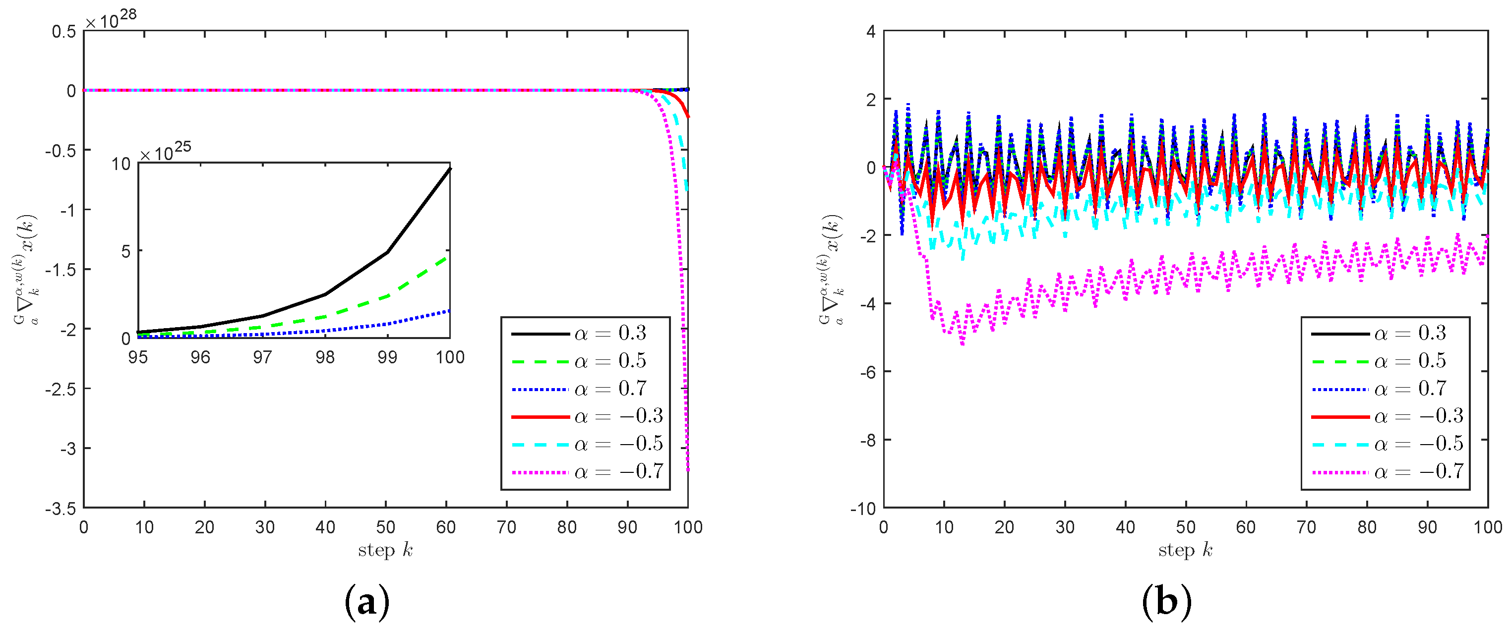
can be calculated. The simulated results are shown are Figure 1.
It can be observed from Figure 1a that a G k α , w ( k ) x ( k ) diverges as k + . More specifically, when α > 0 , the result tends to + . When α < 0 , the result tends to . In this case, a G k α , w ( k ) x ( k ) = i = 0 k a 1 ( i + 1 ) α 1 ¯ Γ ( α ) 2 i sin ( 10 k 10 i ) . Notably, 2 k a 1 + as k + , sin ( 10 k 10 i ) = sin ( 10 ) < 0 when i = k a 1 . If α ( 0 , 1 ) , ( i + 1 ) α 1 ¯ Γ ( α ) < 0 for i N 0 k a 1 . If α ( 1 , 0 ) , ( i + 1 ) α 1 ¯ Γ ( α ) > 0 for i N 0 k a 1 . From this, the trend of a G k α , w ( k ) x ( k ) as k + can be derived. The typical feature of w ( k ) = 0 . 5 k a is that w ( k ) declines rapidly and converges to 0 while the tempered function w ( k ) is assumed to be nonzero. Consequently, a nonzero number is introduced, namely, w ( k ) = 0 . 5 k a + 0.01 . Then, bounded a G k α , w ( k ) x ( k ) follows in Figure 1b. With the increase of k, 0.01 will play a greater role than 0 . 5 k a ; a G k α , w ( k ) x ( k ) performs like a G k α x ( k ) in the steady stage and the tempered case degenerates into the classical case.
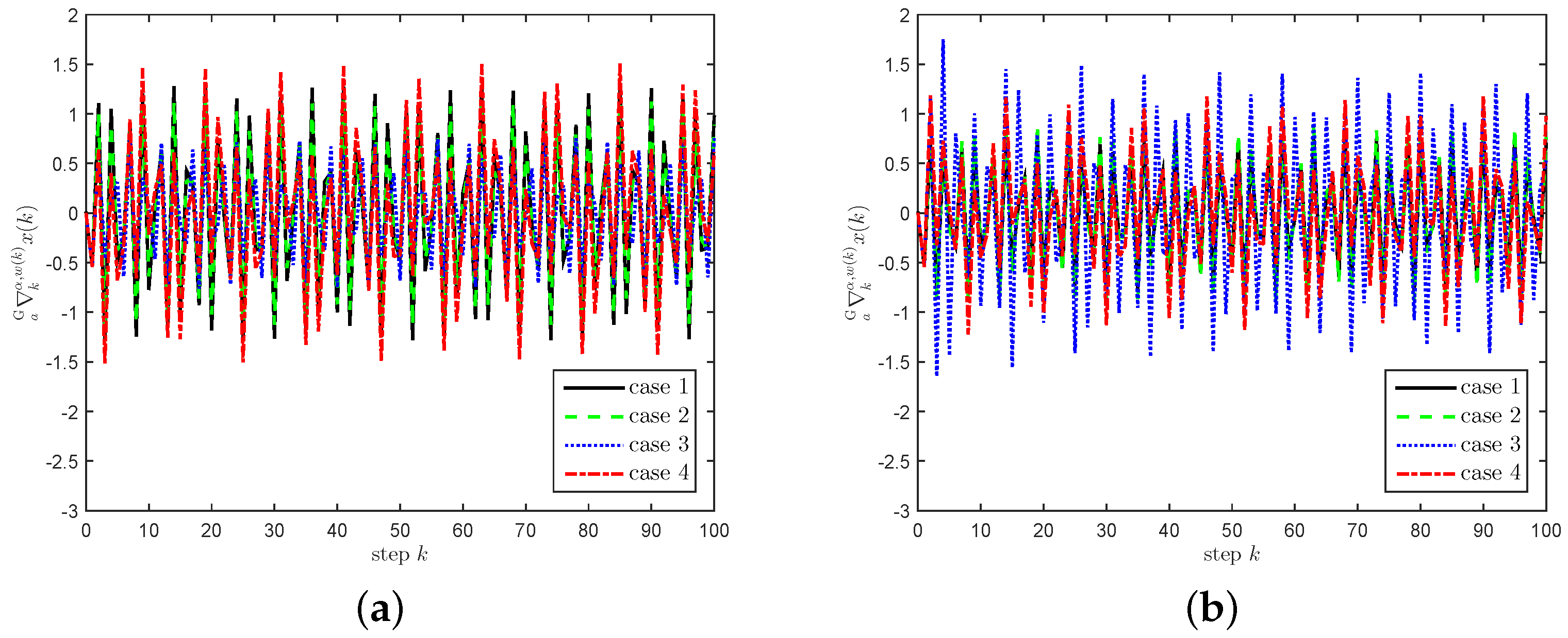
To show more details, the following four cases are considered.
case 1 : w ( k ) = 2 k a ; case 2 : w ( k ) = π k a ; case 3 : w ( k ) = ( 1 ) k a ; case 4 : w ( k ) = sin ( k π 2 a π 2 + π 4 ) .
In each case, w ( k ) enjoys unique properties. In case 1, w ( k ) is positive and monotonically increasing. In case 2, w ( k ) is negative and monotonically decreasing. In case 3, w ( k ) is in oscillation between 1 and 1. Its positive value and negative value appear alternatively. In case 4, w ( k ) is also in oscillation between 2 2 and 2 2 . Two positive values will appear after two negative values. The obtained results are shown in 
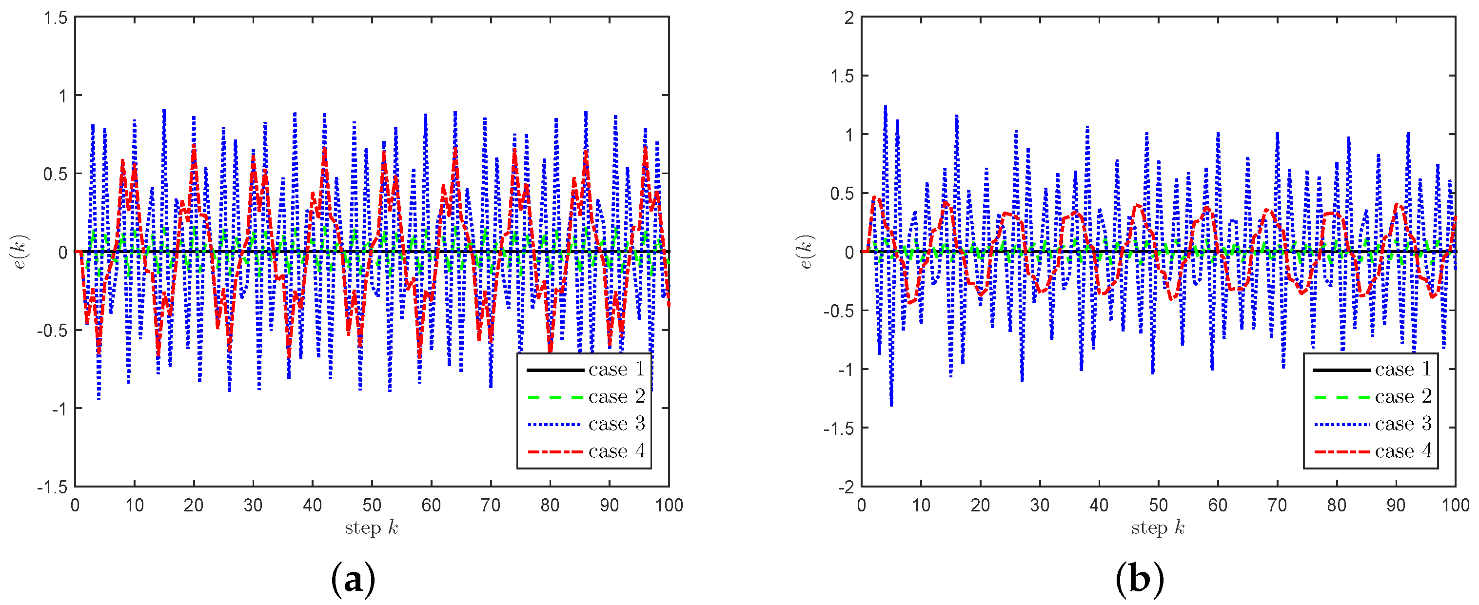
Figure 2. To clearly show the difference, setting case 1 as the standard, the error of a G k α , w ( k ) x ( k ) between each case with the standard is calculated and displayed in Figure 3.
It can be found that, no matter for the fractional difference or the fractional sum, different w ( k ) correspond to different a G k α , w ( k ) x ( k ) in Figure 2. The difference always exists and cannot be ignored. In the same way, different tempered functions can be constructed for different scenarios and satisfy different demands, which could provide great potential to apply nabla tempered fractional calculus.
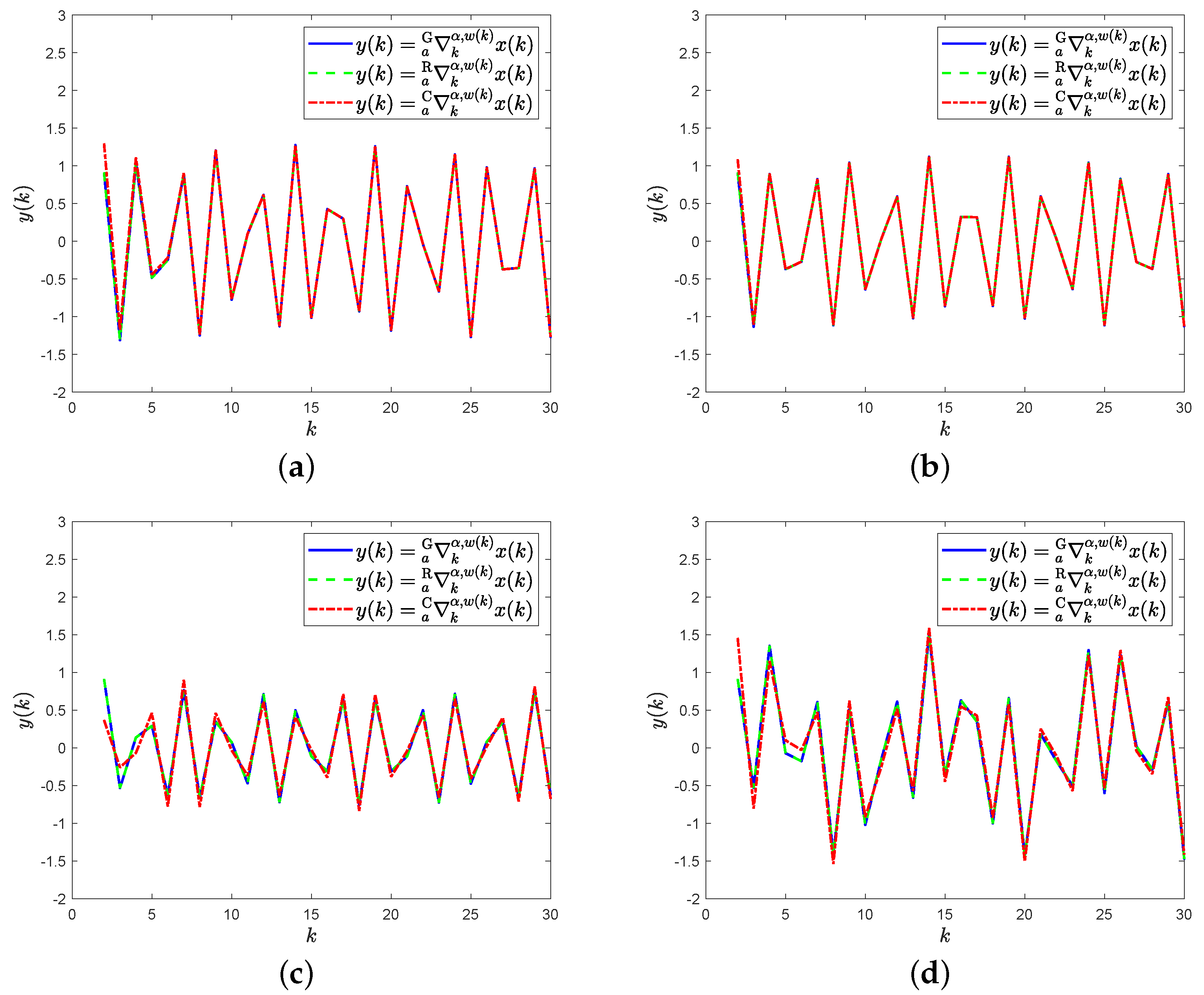
To further check the value of tempered fractional difference, we select x ( k ) = sin ( 10 k ) , α = 0.5 and the aforementioned four cases. The results are shown in Figure 4.
It can be observed that for each w ( k ) , the difference of the three fractional differences is small. From the quantitative analysis, one has
case 1 : 4.4409 × 10 16 a G k α , w ( k ) x ( k ) a R k α , w ( k ) x ( k ) 1.1102 × 10 15 ; case 2 : 8.8818 × 10 16 a G k α , w ( k ) x ( k ) a R k α , w ( k ) x ( k ) 3.3307 × 10 16 ; case 3 : 1.0131 × 10 16 a G k α , w ( k ) x ( k ) a R k α , w ( k ) x ( k ) 4.9960 × 10 16 ; case 4 : 2.2204 × 10 16 a G k α , w ( k ) x ( k ) a R k α , w ( k ) x ( k ) 4.4409 × 10 16 ,
which demonstrates the correctness of Equation (15).

5. Conclusions

This paper constructed a formal mathematical analysis of the nabla tempered fractional difference and fractional sum. A series of analytic properties were developed with rigorous proof including the equivalence relation, the nabla Taylor formula, and the nabla Laplace transform. The developed equivalence relation connects every operator in the class back to the Grünwald–Letnikov, Riemann–Liouville, and Caputo fractional calculi via multiplication and composition. The distinguished results on the nabla Taylor formula give the equivalent description for the nabla tempered fractional difference/sum, which could be helpful for analyzing and computing. The results on the nabla Laplace transform bridge the connection between the time–domain property and the frequency–domain property of the nabla tempered fractional difference/sum. All these results help to establish a firm foundation for the theory of nabla tempered fractional calculus. The current work is purely theoretical, but much remains to be done in the direction of nabla tempered fractional difference equations and applications. It is believed that this work reveals the relationship between time domain and frequency domain of nabla tempered fractional calculus and enriches the knowledge of nabla tempered fractional calculus.
Future work following this paper may include the following interesting topics.
(i)
Explore the properties of nabla tempered fractional calculus with respect to functions;
(ii)
Discuss the numerical approximation of nonlinear nabla tempered fractional equations;
(iii)
Develop and evaluate the essential inequalities on nabla tempered fractional calculus.

Author Contributions

Writing–original draft, Y.W.; Formal analysis, L.Z.; Validation, X.Z.; Investigation, J.C. All authors have read and agreed to the published version of the manuscript.

Funding

The work described in this paper was funded by the National Natural Science Foundation of China (62273092, 61833005, U22B2046), the National Key R&D Project of China (2020YFA0714300), the Fundamental Research Funds for the Central Universities (4007012302) and ZhiShan Youth Scholar Program of SEU.

Institutional Review Board Statement

Not applicable.

Informed Consent Statement

Not applicable.

Data Availability Statement

Not applicable.

Conflicts of Interest

The authors declare no conflict of interest.

References

  1. Wang, Y.Y.; Sun, H.G.; Fan, S.Y.; Gu, Y.; Yu, X.N. A nonlocal fractional peridynamic diffusion model. Fractal Fract. 2021, 5, 76. [Google Scholar] [CrossRef]
  2. Diethelm, K.; Kiryakova, V.; Luchko, Y.; Machado, J.A.T.; Tarasov, V.E. Trends, directions for further research, and some open problems of fractional calculus. Nonlinear Dyn. 2022, 107, 3245–3270. [Google Scholar] [CrossRef]
  3. Atıcı, F.M.; Chang, S.; Jonnalagadda, J. Grünwald–Letnikov fractional operators: From past to present. Fract. Differ. Calc. 2021, 11, 147–159. [Google Scholar] [CrossRef]
  4. Agrawal, O.P. Some generalized fractional calculus operators and their applications in integral equations. Fract. Calc. Appl. Anal. 2012, 15, 700–711. [Google Scholar] [CrossRef]
  5. Cao, J.X.; Li, C.P.; Chen, Y.Q. On tempered and substantial fractional calculus. In Proceedings of the IEEE/ASME 10th International Conference on Mechatronic and Embedded Systems and Applications, Senigallia, Italy, 10–12 September 2014; pp. 1–6. [Google Scholar] [CrossRef]
  6. Sabzikar, F.; Meerschaert, M.M.; Chen, J.H. Tempered fractional calculus. J. Comput. Phys. 2015, 293, 14–28. [Google Scholar] [CrossRef] [PubMed] [Green Version]
  7. Mali, A.D.; Kucche, K.D.; Fernandez, A.; Fahad, H.M. On tempered fractional calculus with respect to functions and the associated fractional differential equations. Math. Methods Appl. Sci. 2022, 17, 12–27. [Google Scholar] [CrossRef]
  8. Obeidat, N.A.; Rawashdeh, M.S. Theories of tempered fractional calculus applied to tempered fractional Langevin and Vasicek equations. Math. Methods Appl. Sci. 2023. [Google Scholar] [CrossRef]
  9. Fernandez, A.; Ustaoglu, C. On some analytic properties of tempered fractional calculus. J. Comput. Appl. Math. 2020, 366, 112400. [Google Scholar] [CrossRef] [Green Version]
  10. Fernandez, A.; Fahad, H.M. Weighted fractional calculus: A general class of operators. Fractal Fract. 2022, 6, 208. [Google Scholar] [CrossRef]
  11. Kucche, K.D.; Mali, A.D.; Fernandez, A.; Fahad, H.M. On tempered Hilfer fractional derivatives with respect to functions and the associated fractional differential equations. Chaos Solitons Fractals 2022, 163, 112547. [Google Scholar] [CrossRef]
  12. Gu, C.Y.; Zheng, F.X.; Shiri, B. Mittag–Leffler stability analysis of tempered fractional neural networks with short memory and variable-order. Fractals 2021, 29, 2140029. [Google Scholar] [CrossRef]
  13. Ortigueira, M.D.; Bengochea, G.; Machado, J.T. Substantial, tempered, and shifted fractional derivatives: Three faces of a tetrahedron. Math. Methods Appl. Sci. 2021, 44, 9191–9209. [Google Scholar] [CrossRef]
  14. Almeida, R.; Morgado, M.L. Analysis and numerical approximation of tempered fractional calculus of variations problems. J. Comput. Appl. Math. 2019, 361, 1–12. [Google Scholar] [CrossRef]
  15. Xie, C.X.; Xia, X.X.; Aghdam, Y.E.; Farnam, B.; Jafari, H.; Wang, S.C. The numerical strategy of tempered fractional derivative in European double barrier option. Fractals 2022, 30, 2240049. [Google Scholar] [CrossRef]
  16. Rayal, A.; Verma, S.R. Two-dimensional Gegenbauer wavelets for the numerical solution of tempered fractional model of the nonlinear Klein–Gordon equation. Appl. Numer. Math. 2022, 174, 191–220. [Google Scholar] [CrossRef]
  17. Abdeljawad, T.; Banerjee, S.; Wu, G.C. Discrete tempered fractional calculus for new chaotic systems with short memory and image encryption. Optik 2020, 218, 163698. [Google Scholar] [CrossRef]
  18. Fu, H.; Huang, L.L.; Abdeljawad, T.; Luo, C. Tempered fractional calculus on time scale for discrete-time systems. Fractals 2021, 29, 2140033. [Google Scholar] [CrossRef]
  19. Ferreira, R.A.C. Discrete weighted fractional calculus and applications. Nonlinear Dyn. 2021, 104, 2531–2536. [Google Scholar] [CrossRef]
  20. Wei, Y.H.; Chen, Y.Q.; Wei, Y.D.; Zhao, X. Lyapunov stability analysis for nonlinear nabla tempered fractional order systems. Asian J. Control. 2022. [Google Scholar] [CrossRef]
  21. Cheng, J.F. Fractional Difference Equation Theory; Xiamen University Press: Xiamen, China, 2011. [Google Scholar]
  22. Ostalczyk, P. Discrete Fractional Calculus: Applications in Control and Image Processing; World Scientific Publishing Company: Berlin, Germany, 2015. [Google Scholar]
  23. Goodrich, C.; Peterson, A.C. Discrete Fractional Calculus; Springer: Cham, Switzerland, 2015. [Google Scholar]
  24. Ferreira, R.A.C. Discrete Fractional Calculus and Fractional Difference Equations; Springer: Cham, Switzerland, 2022. [Google Scholar]
  25. Cheng, J.F. Non-Uniform Lattice Based Hypergeometric Equations and Fractional Difference Sums; Science Press: Beijing, China, 2022. [Google Scholar]
  26. Wei, Y.H.; Gao, Q.; Liu, D.Y.; Wang, Y. On the series representation of nabla discrete fractional calculus. Commun. Nonlinear Sci. Numer. Simul. 2019, 69, 198–218. [Google Scholar] [CrossRef]
  27. Wei, Y.H.; Chen, Y.Q.; Wang, Y.; Chen, Y.Q. Some fundamental properties on the sampling free nabla Laplace transform. In Proceedings of the ASME 2019 International Design Engineering Technical Conferences & Computers and Information in Engineering Conference, Anaheim, CA, USA, 18–21 August 2019. [Google Scholar] [CrossRef] [Green Version]
  28. Wei, Y.H.; Yin, W.D.; Zhao, Y.T.; Wang, Y. A new insight into the Grünwald–Letnikov discrete fractional calculus. J. Comput. Nonlinear Dyn. 2019, 14, 041008. [Google Scholar] [CrossRef]
  29. Li, C.P.; Deng, W.H. Remarks on fractional derivatives. Appl. Math. Comput. 2007, 187, 777–784. [Google Scholar] [CrossRef]
  30. Almeida, R. Further properties of Osler’s generalized fractional integrals and derivatives with respect to another function. Rocky Mt. J. Math. 2019, 49, 2459–2493. [Google Scholar] [CrossRef]
  31. Wei, Y.Q.; Liu, D.Y.; Boutat, D.; Liu, H.R.; Wu, Z.H. Modulating functions based model-free fractional order differentiators using a sliding integration window. Automatica 2021, 130, 109679. [Google Scholar] [CrossRef]
Figure 1. Time evolution of a G k α , w ( k ) x ( k ) : (a) w ( k ) = 0 . 5 k a ; (b) w ( k ) = 0 . 5 k a + 0.01 .
Fractalfract 07 00330 g001
Figure 2. Time evolution of a G k α , w ( k ) x ( k ) : (a) α = 0.5 ; (b) α = 0.5 .
Fractalfract 07 00330 g002
Figure 3. The error of a G k α , w ( k ) x ( k ) in different cases: (a) α = 0.5 ; (b) α = 0.5 .
Fractalfract 07 00330 g003
Figure 4. Time evolution of a G k α , w ( k ) x ( k ) , a R k α , w ( k ) x ( k ) and a C k α , w ( k ) x ( k ) : (a) w ( k ) = 2 k a ; (b) w ( k ) = π k a ; (c) w ( k ) = ( 1 ) k a ; (d) w ( k ) = sin ( k π 2 a π 2 + π 4 ) .
Fractalfract 07 00330 g004
Disclaimer/Publisher’s Note: The statements, opinions and data contained in all publications are solely those of the individual author(s) and contributor(s) and not of MDPI and/or the editor(s). MDPI and/or the editor(s) disclaim responsibility for any injury to people or property resulting from any ideas, methods, instructions or products referred to in the content.

