Article

Multiplicative Noise Removal and Contrast Enhancement for SAR Images Based on a Total Fractional-Order Variation Model

School of Mathematics, Harbin Institute of Technology, Harbin 150001, China
*
Author to whom correspondence should be addressed.
Fractal Fract. 2023, 7(4), 329; https://doi.org/10.3390/fractalfract7040329
Submission received: 21 March 2023 / Revised: 10 April 2023 / Accepted: 10 April 2023 / Published: 14 April 2023

Abstract

:
In this paper, we propose a total fractional-order variation model for multiplicative noise removal and contrast enhancement of real SAR images. Inspired by the high dynamic intensity range of SAR images, the full content of the SAR images is preserved by normalizing the original data in this model. Then, we propose a degradation model based on the nonlinear transformation to adjust the intensity of image pixel values. With MAP estimator, a corresponding fidelity term is introduced into the model, which is beneficial for contrast enhancement and bias correction in the denoising process. For the regularization term, a gray level indicator is used as a weighted matrix to make the model adaptive. We first apply the scalar auxiliary variable algorithm to solve the proposed model and prove the convergence of the algorithm. By virtue of the discrete Fourier transform (DFT), the model is solved by an iterative scheme in the frequency domain. Experimental results show that the proposed model can enhance the contrast of natural and SAR images while removing multiplicative noise.

1. Introduction

Digital images are often affected by various external physical conditions during the processes of storage, transmission, and transformation, resulting in quality degradation, which not only affects the visualization of images, but also causes difficulties in the subsequent processing and application of the image. Therefore, image denoising has always been a hot research topic in image processing [1]. Noise in images can be roughly divided into two categories: additive noise and multiplicative noise. In the past few decades, research on removing additive noise has been extensive and mature. Unlike additive noise, multiplicative noise, which commonly appears in SAR images, laser images, ultrasound images, and positron emission tomography (PET), is signal independent, non-Gaussian, and spatially dependent [2,3,4,5]. One of the most important tasks for this image denoising problem is that details such as edges and textures should be efficiently kept while restoring the degraded image. Since this course lacks some prior information, it is a classic ill-posed problem. In this problem, we are interested in degraded image f : Ω R arising from original images u by corruption with (uncorrelated) multiplicative noise η of mean 1, i.e.,
f = u η .
Here, η follows a Gamma distribution and the probability density function (PDF) of Gamma noise is
p η ( x ; θ , K ) = 1 θ K Γ ( K ) x K 1 e x θ
where Γ ( · ) is Gamma function, θ is scale parameter, and K is shape parameter. Furthermore, the mean of η is K θ and the variance of η is K θ 2 . In general, we assume that the mean of η is equal to 1, then we obtain K θ = 1 and its variance of 1 K . The objective of image denoising is to find the unknown true image u from a degraded image f.
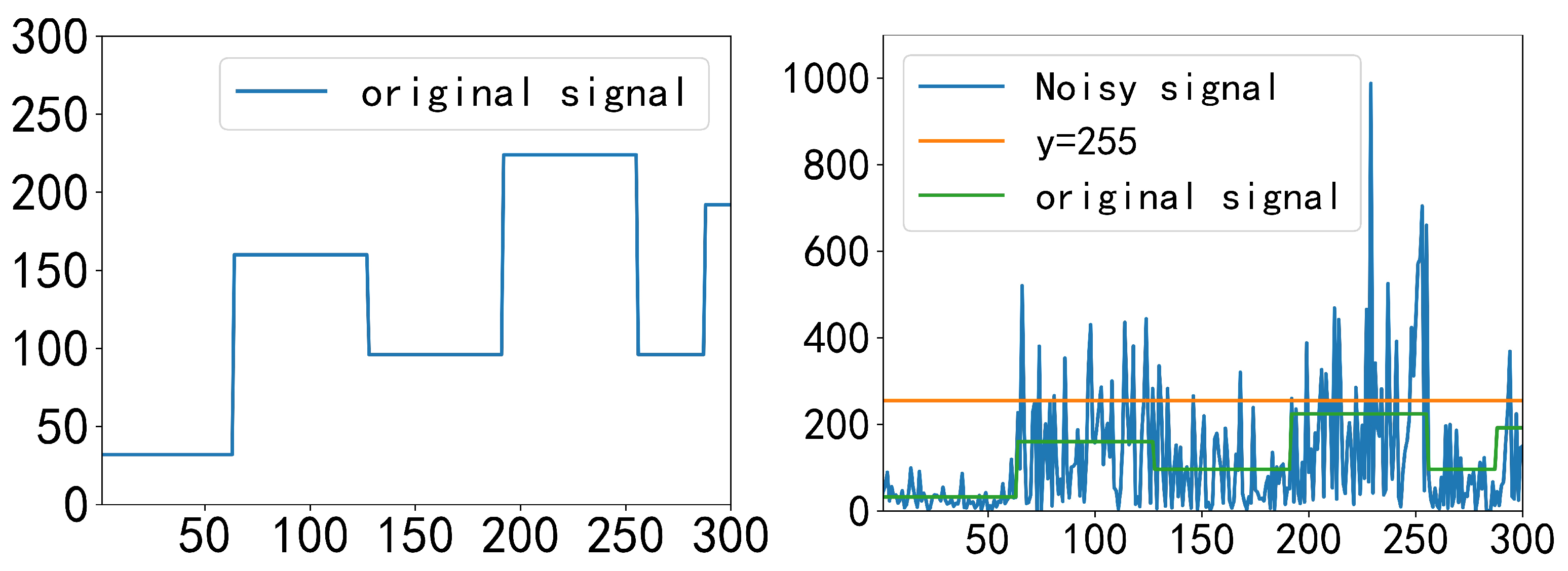
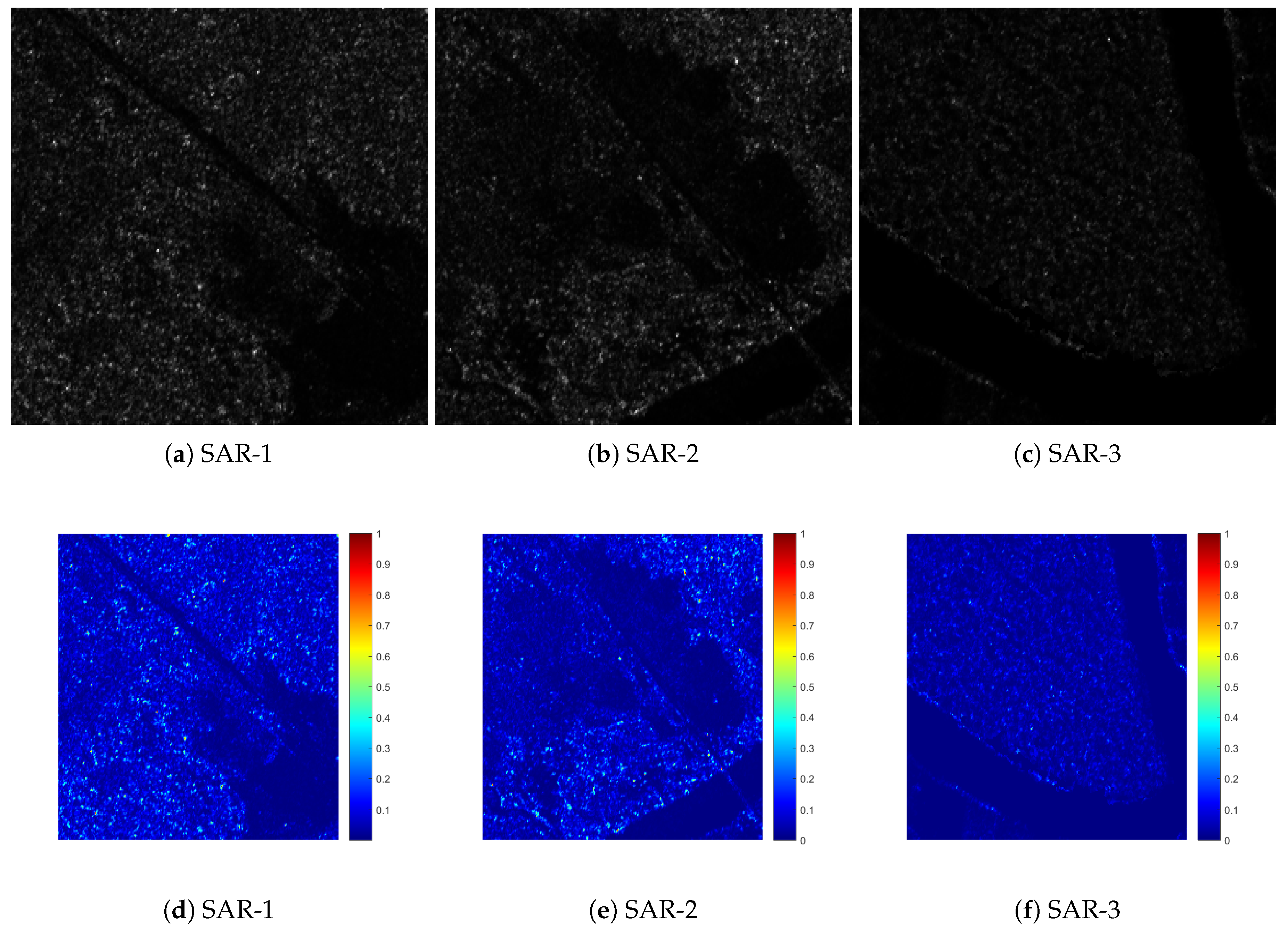
In order to investigate the effect of degradation, we discriminate differences in the strength of one-dimensional Gamma noise in Figure 1. For optical images, it shows that the intensity value of the degraded signal usually has a higher intensity range compared to the original signal. Unlike the imaging acquisition processes of optical images, the pixel range of SAR images is usually much larger [6]. Specifically, SAR image data are highly accurate and usually have a bit depth of 16 bits, 24 bits, or higher [7]. However, the existing multiplicative denoising models often use a truncation function in the denoising process to fix the pixel values of the image in a certain fixed range, which is obviously not suitable for the denoising process of SAR images. Traditional linear histogram rescaling is a good choice for image visualization; however, this simple linear shrinkage can cause significant information loss due to the long distribution tails and the associated concentration on low raw values [8]. To overcome these shortcomings, researchers have proposed more innovative SAR image dynamic range compression algorithms, such as image compression algorithms based on hierarchical image fusion and image compression algorithms based on nonlinear transformation [9,10]. These algorithms have solved the problems of linear dynamic range compression algorithms to a certain extent, but they still have the defects of detail loss and poor adaptive processing ability [11]. Since existing models usually use a truncation function to map the intensity values of the recovered images to [ 0 , 255 ] during denoising, this will reduce the purity of the edge/texture information in the SAR images [12,13]. Therefore, the variation of intensity range should also be taken into account when denoising multiplicative noise.
To remove multiplicative noise from SAR images, many multiplicative denoising models have been proposed, among which the variational models based on total variation (TV) regularization have achieved impressive results, as the space of total variation exhibits jump discontinuities [12,13,14,15]. In 2008, the AA model was designed to solve the degradation model f = u η , the process of image reconstruction was formulated into the maximum a posteriori (MAP) framework [12]. With MAP estimator, the model for restoring images corrupted with Gamma noise was proposed as
inf u B V ( Ω ) E ( u ) = λ Ω log   u + f u + J ( u ) ,
where f is the corrupted image and J ( u ) stands for the total variation of u. The fidelity term H ( u , f ) = Ω log   u + f u d x is strictly convex for u ( 0 , 2 f ) . The parameter λ is used to balance the influence of these two terms. Although the optimization problem is nonconvex, Aubert and Aujol showed the existence of minimizers of the optimization problem under certain conditions. For the reason that the AA model is nonconvex, the methods mentioned may stick at some local minimizers. To overcome these problems, Shi and Osher [16] transformed the multiplicative denoising problem into an additive denoising problem by considering a noisy observation given by log   f = log   u + log   η , then they turn the denoising model into a convex model by adopting the fidelity term. In [13], Dong and Zeng added a penalty term Ω u f 1 2 d x to the AA model by virtue of the statistical properties of the multiplicative Gamma noise; the model is as follow:
inf u S ( Ω ) Ω log   u + f u d x + α Ω u f 1 2 d x + λ Ω D u ,
which is global convex when the equilibrium parameters meet certain conditions. However, the variational models based on total variation (TV) regularization often yield the staircase effects and the loss of image contrasts [17].
To overcome the weakness of variational models based on the TV model, nonlinear diffusion equation methods were also widely studied. Two types of nonlinear diffusion equation methods have been proposed in the literature. The first type introduces the nonlinear diffusion equation of its integer order; for example, the speckle-reducing anisotropic diffusion (SRAD) models [18,19] were proposed by modifying the diffusion coefficients to deal with various noise distributions. In 2015, Zhou et al. proposed a nonlinear diffusion filter denoising framework which was named the DD model [20]. They considered not only the information of the gradient of the image, but also the information of gray levels of the image; the diffusion model is shown as follow:
u t = div a ( | u | , u ) | u | λ H ( u , f ) , o n Ω × ( 0 , T ) , u , n = 0 , o n Ω × ( 0 , T ) , u ( x , y , 0 ) = f ( x , y ) , o n Ω ,
where the parameter λ balances the fidelity term and the regularization term. In this model, a particular case was chosen under the framework of the diffusion equation, i.e., they took H ( u , f ) = 0 . The coefficient a ( | u | , u ) = b ( u ) c ( | u | ) was divided into two independent parts, where b ( u ) is a function of the gray level of u and c ( | u | ) is a function of the gradient | u | . Inspired by the DD model, a gray level indicator-based nonlinear telegraph diffusion model is also presented for image despeckling, which successfully preserves the image edges during the noise removal process [21]. The mentioned models often use information such as first-order differential operators or second-order Hessian matrices to detect image gray value changes at the discrete level using neighboring pixel points, and thus the obtained results are local in nature. Since the image texture structure is usually non-local in nature, the image texture structure obtained by existing first- or second-order denoising models is usually easily blurred.
Unlike the integer-order operator, the fractional-order differential operator is a nonlocal operator [22,23] which can achieve texture detection by inductively obtaining the autocorrelation of an image with different weight coefficients based on the proximity relationship between individual pixel points of the image. Therefore, the second type introduces the nonlinear diffusion equations of their fractional-order derivative, which can be seen as the generalization of the integer-order derivative. In [24], Bai and Feng introduced a fractional-order anisotropic diffusion model to remove additive noise (BF model), which is shown as follow:
u t = D x α * c D α u D α u D y α * c D α u D α u ,
where D x α * is the adjoint of D x α and D y α * is the adjoint of D y α . This model can be seen as generalizations of second-order and fourth-order anisotropic diffusion equations, because (4) turned into the Perona–Malik model when α = 1 and the fourth-order anisotropic diffusion model when α = 2 . With 1 < α < 2 , the BF model exhibited higher perceptual quality than second-order and fourth-order PDEs. The diffusion equations can be seen as the Euler–Lagrange equations of an increasing energy function of the absolute value of the fractional derivative, but the energy minimization models are not studied in that way; in other words, the model lacks some theoretical analysis. In order to analyze properties of the total α -order variation, Zhang and Chen proposed a fractional-order derivative-based total α -order variation model which provides the foundation for applications in imaging inverse problems as a regularization term [25]. Due to the strong denoising capability of the fractional-order diffusion models, fractional-order derivatives are also used in the removal of multiplicative noise. In [26], a fractional-order nonlinear diffusion model based on adaptive anisotropic fractional diffusion equations (AAFD) was proposed to denoise the texture images corrupted by multiplicative noise; the model is as follows:
u t = D x α * | u | M r 1 1 + k | D α u | β D x α D y α * | u | M r 1 1 + k | D α u | β D y α , u ( x , y , t ) = 0 , o n Ω × ( 0 , T ) , u ( x , y , 0 ) = f ( x , y ) , o n Ω ,
where 0 < α < 2 , 0 < β < 1 and M = sup ( x , y ) Ω u . By adjusting the parameter α , the fractional-order derivative performs well both in accommodating the texture details and eliminating the staircase effect.
To the best of our knowledge, most of the aforementioned work does not take into account the variation in the range of values of SAR images during denoising. In addition, we always compute a smooth solution in Sobolev spaces [24,26,27]. Thus, smoothing (by local weighted averaging) is an effective image regularization method that has been used for denoising [24]. However, SAR images should not be smoothed too much, because the studies on discriminating between SAR clutter textures are important [28,29]. Therefore, to better preserve image texture details, the natural space for our computational solution is B V α ( Ω ) , i.e., the space of functions with bounded variation. When dealing with strong Gamma noise, a truncation function is used to confirm the intensity values to be in [ 0 , 255 ] . Regrettably, especially for SAR images, image structure and information would be terribly damaged with the fixed intensity range. Due to the fact that plenty of models were proposed to remove the multiplicative noise without considering the real range and information loss of the restored images, a gray value adjustment is essential in the noise removal process.
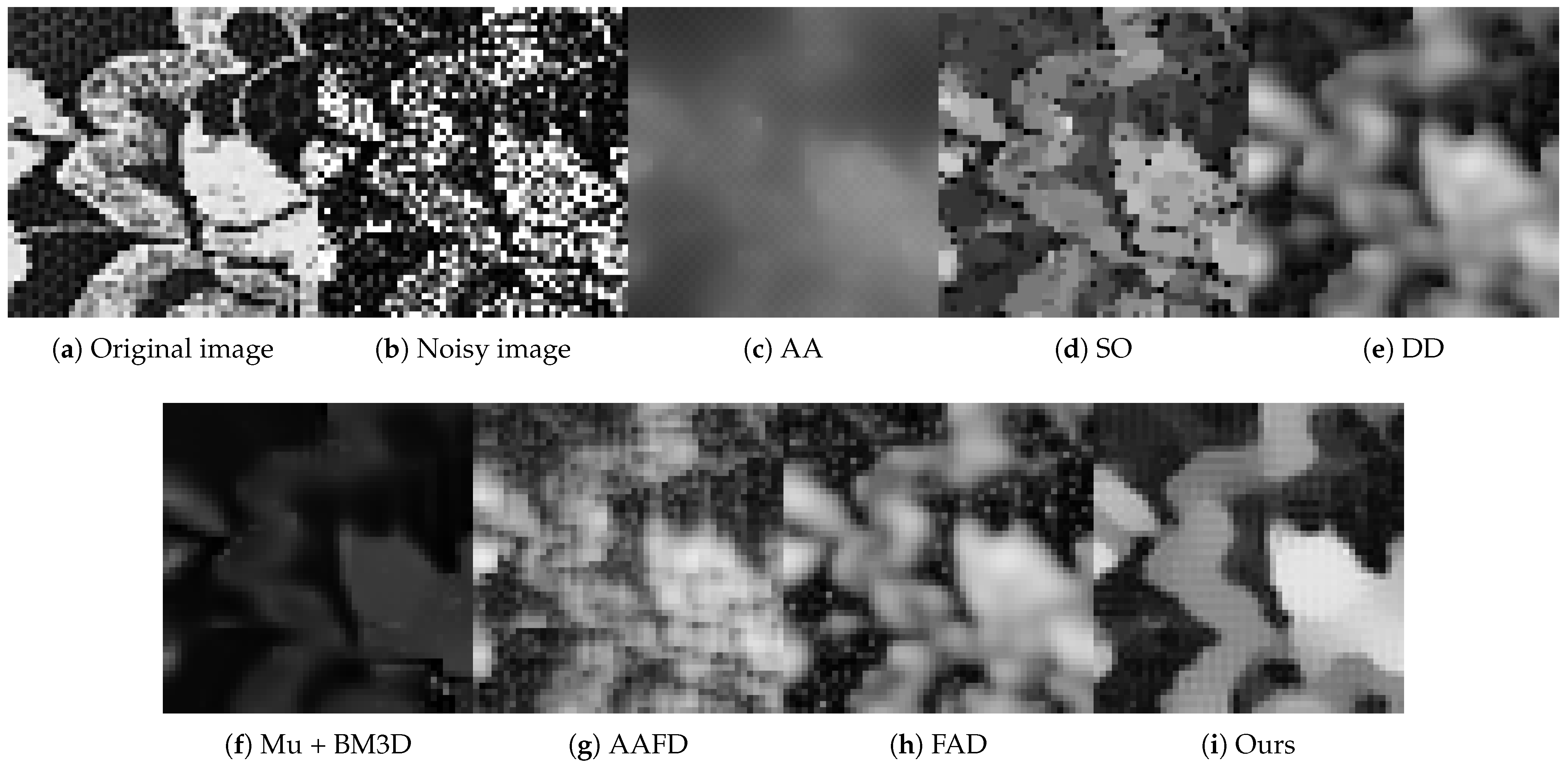
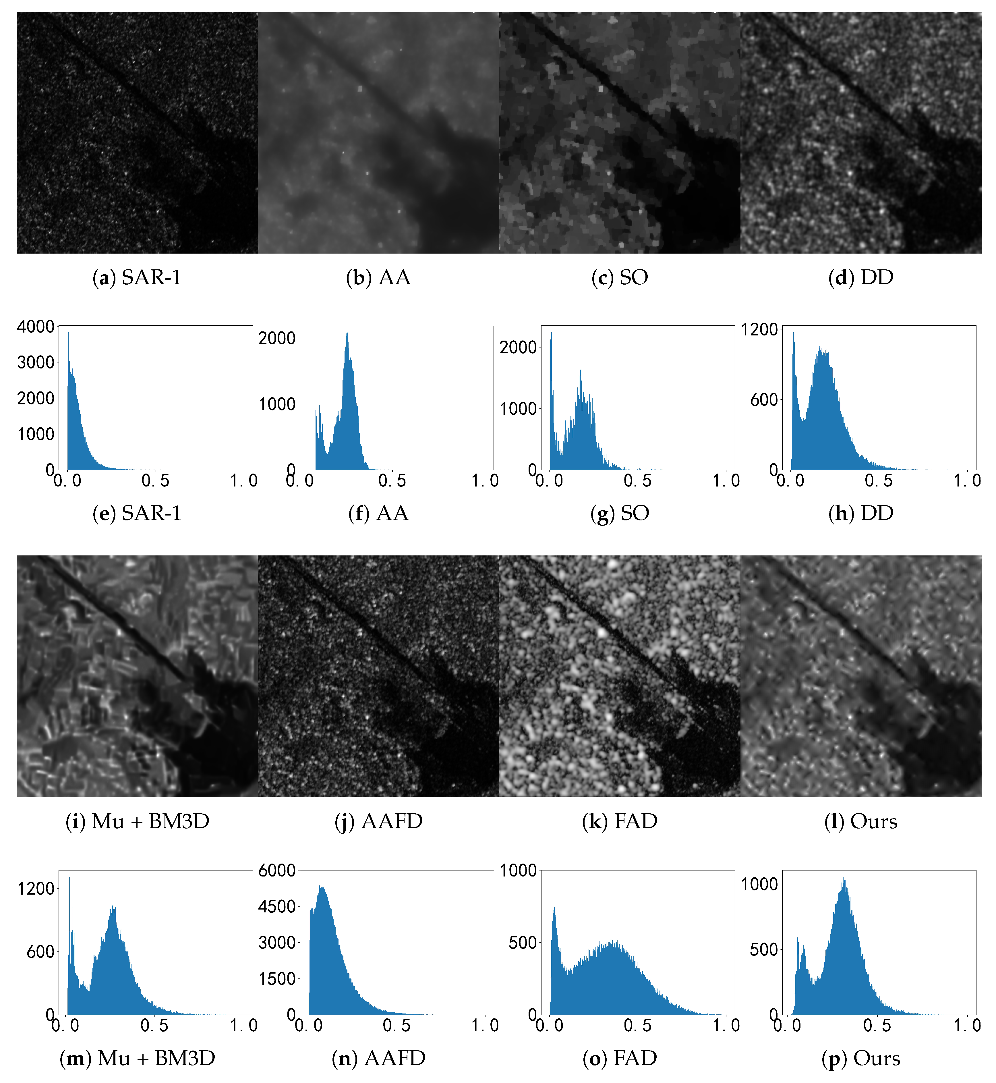
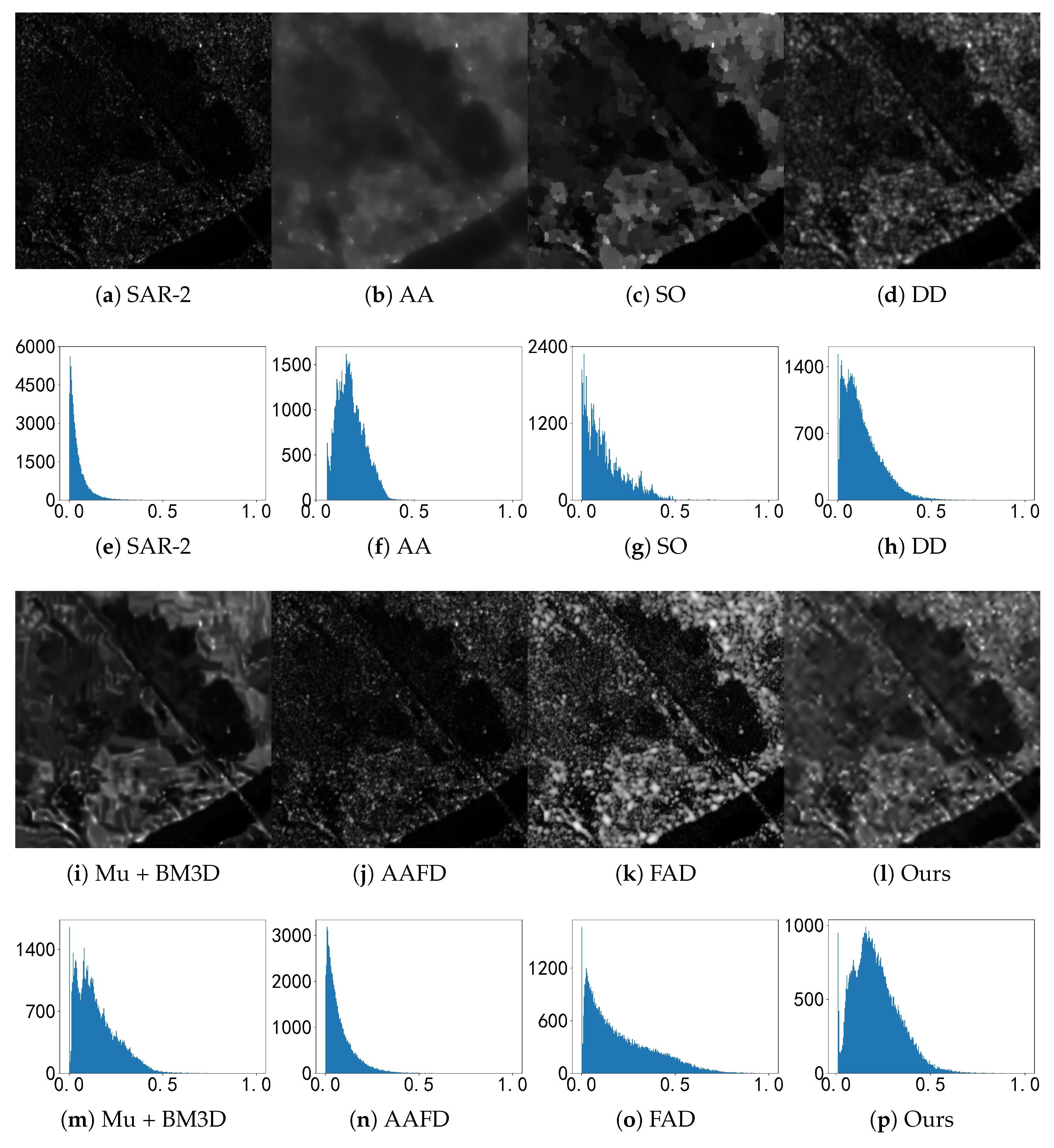
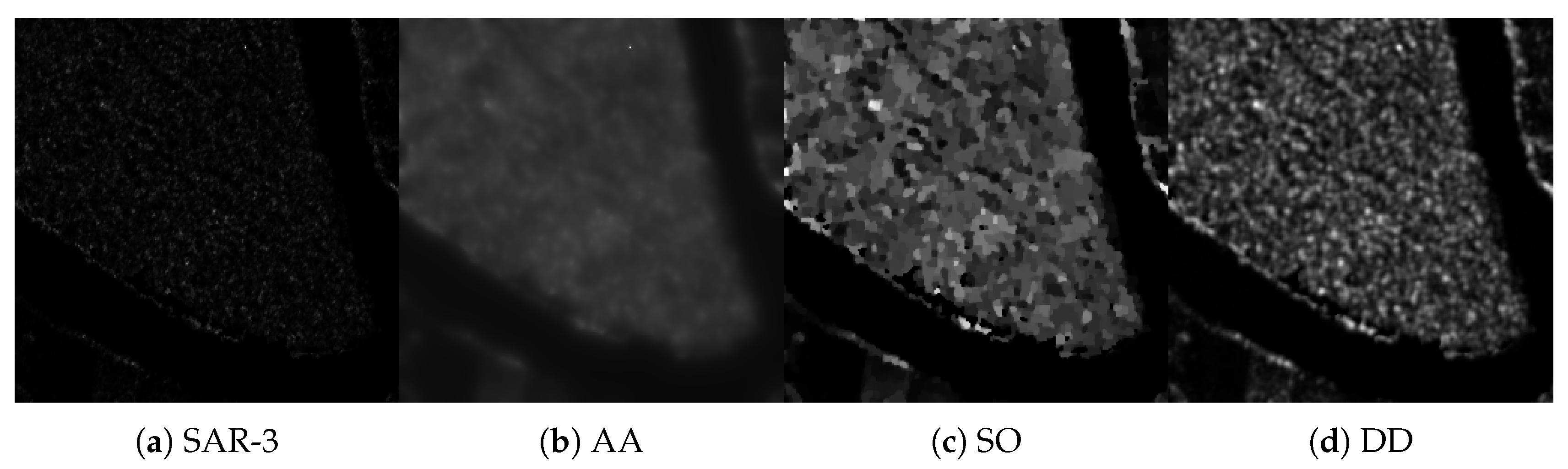
In this paper, we aim to remove multiplicative noise from three real SAR datasets in range [ 0 , 1 ] . Because noise-free SAR images do not exist, we cannot calculate the PSNR and MAE. To solve this problem, degraded aerial and texture images are normalized to simulate real SAR images. Then, we propose a fractional-order variational denoising enhancement model based on a nonlinear transformation that is effective in both texture enhancement and noise removal. A lot of models are built on the inverse problem f max ( f ) = u max ( f ) η [12,26,27], then the denoising result of u [ 0 , 1 ] is obtained. However, max ( f ) is unknown as the Gamma noise is random, and u × max ( f ) usually exceeds the displayable range of a normal image. We aim to visualize the denoised result u more effectively. Thus, we proposed a degradation model based on the nonlinear transformation to adjust the intensity of image pixel value. The fractional-order variational model proposed in this paper was built on this new degradation model. Considering the gray scale, visualizing the denoising results to the range of [ 0 , 255 ] by u × 255 is a suitable choice. Compared with the restored result u × max ( f ) , a bias correction is also introduced into the proposed denoising model to overcome the accuracy problem. The existing integer-order operator uses adjacent pixel points to detect the change in image gray value in the process of numerical discretization, which is local in nature and is only applicable to dealing with local features, such as image edges, and cannot effectively deal with non-local texture features. Due to the non-locality, self-similarity, and long-range dependence property of fractional-order differential operators, an adaptive fractional-order regularization term is proposed in this paper to protect the texture features of images.

Contributions

In this paper, we introduce a new degraded model with a nonlinear transformation. Following the MAP estimator for multiplicative Gamma noise, a corresponding fidelity term is obtained. Unlike many denoising models, we focus on information preservation and detail enhancement for real SAR images or other images with high-intensity dynamic range. Inspired by this issue, a total fractional-order variation model is proposed to preserve and enhance the image textures. In this model, we do not use the truncation function to force the intensity values of restored images between 0 and 255.
(i)
A new degraded model is proposed in order to obtain the restored result in a proper range from the normalized degraded images, then the corresponding fidelity term is introduced, which is used to enhance the restored images and show more local details.
(ii)
We consider the framework of total fractional-order variation model with adaptive regularization term for texture image multiplicative noise removal.
(iii)
The proposed total fractional-order variation model is nonconvex, so a good initialization will be helpful to obtain a satisfactory result. Thus, we give more flexible initialization choices by tuning magnitude characteristics and reach a compromise between sensitivity to noise and detection accuracy.
(iv)
The noise removal model is firstly solved by the scalar auxiliary variable approach, and the obtained experimental results are satisfied.
The rest of the paper is organized as follows. In Section 2, some related models for multiplicative noise removal are briefly described. In Section 3, the new degraded model aiming to enhance the detail of restored images is proposed, then we introduce the fidelity term by using a maximum a posteriori (MAP) estimator. After that, we propose a total fractional-order variation model with a gray level indicator, and the properties of solutions to functional minimization are also demonstrated. In Section 4, the scalar auxiliary variable approach is used to solve the minimization problem. In Section 5, some numerical experiments are given to illustrate the performance of the proposed algorithm. In Section 6, concluding remarks are given.

2. Related Methods

In this section, we give a review of the total α -order variation model and the fractional-order anisotropic diffusion model, which motivate us to develop a new fractional-order variation model for removing the multiplicative noise from SAR images.

2.1. α -TV Model

To mitigate the weakness of a total variation-based model for image restoration, Zhang and Chen proposed a total α -order variation model in [25]. Furthermore, they first reviewed some results of fractional-order derivatives and then analyzed the theoretical properties of the proposed total α -order variational model rigorously; the model is as follow:
inf u B V α ( Ω ) { T V α ( u ) + λ 2 Ω | u f | 2 d x } ,
where Ω = ( 0 , 1 ) × ( 0 , 1 ) R 2 and 1 < α < 2 . This model was designed in B V α ( Ω ) space, which denotes the space of bounded variation functions. B V α ( Ω ) space is the subspace of functions u L 1 ( Ω ) , and the space of functions of B V α ( Ω ) is further defined by
B V α ( Ω ) : = { u L 1 ( Ω ) | T V α ( u ) < } ,
where T V α ( u ) : = sup ϕ K Ω u d i v α ϕ d x and K = : { ϕ C 0 l ( Ω , R n ) , | ϕ ( x ) | 1 , x Ω } . The convexity, the solvability, and a solution theory for the total α -order variation model is also established, which makes it more advantageous to work with than high-order and nonconvex counterparts (such as a mean curvature-based model).
The α T V model did well in removing additive noise and preserve image detail from non-texture images with clear edges. Unlike additive noise, multiplicative noise is signal independent, non-Gaussian, and spatially dependent, i.e., variance is a function of signal amplitude. Inspired by the α T V model, we proposed a total fractional-order variation model for multiplicative noise removal and contrast enhancement in real SAR images. According to the properties of multiplicative noise and the task for image detail enhancement, we try to propose a new degraded model. Following this degraded model, a new fidelity term is proposed under the framework of MAP estimator.

2.2. FAD Model

In [27], Shan et al. applied the fractional Fick’s law to the framework of the diffusion model for image processing (two-dimension task). Based on the comprehensive physical background of the fractional Fick’s law, they proposed a fractional-order anisotropic diffusion model for multiplicative noise removal in texture-rich images, which is as follows:
u t = · q ( x , y , t ) , i n Ω × ( 0 , T ) , u ( x , y , t ) = 0 , o n Ω × ( 0 , T ) , u ( x , y , 0 ) = f ( x , y ) , o n Ω ,
where Ω = [ a , b ] × [ c , d ] R 2 and = ( x , y ) . The diffusion flux q ( x , y , t ) = ( q x , q y ) is defined by
q x = c ( u , D x + α u ) D x + α u + c ( u , D x α u ) D x α u ,
q x = c ( u , D y + α u ) D y + α u + c ( u , D y α u ) D y α u ,
where 0 < α < 3 , D x + α , D x α , D y + α , D y α are the left and right Riemann–Liouville fractional derivatives. The diffusion coefficient is defined as c ( u , | · | ) = G σ u max ( G σ u ) β · 1 1 + γ | · | , where β and γ are both positive constants and G σ is a convolution with a Gaussian kernel.
In this model, the diffusion coefficient involved not only the information of gray levels of the image, but also the gradient of the image. Let c ( u , | α u | ) = a ( u ) b ( | α u | ) , then a ( u ) takes into account the gray level of the noisy image and controls the speed of diffusion at different regions. b ( | α u | ) is used as a texture detection function and possesses the similar form of the edge detection function ( b ( | α u | ) would be small in the edge) in the PM model. Compared with the traditional fractional-order diffusion model, the FAD model performs well both in removing multiplicative noise and keeping texture. However, the edge detection function would also be small when the image is degraded by strong multiplicative noise, so both the texture and noise would be preserved. For this reason, we design the same gray indicator, which takes into account the information of gray levels of the image under the new degraded model. The gray indicator can also be seen as a weighting function, and the information of gray levels controls the speed of diffusion at different regions; the speed is slow at the low gray level, and the speed is fast at the high gray level.

3. The Proposed Multiplicative Noise Removal Model with Contrast Enhancement

In this section, we introduce a new degradation model. Based on the Bayes rule, we construct the fidelity term by using a maximum a posteriori (MAP) estimator. Then, an adaptive fractional-order regularization term is proposed for the fractional-order operator, which is nonlocal and useful to preserve the texture details of the image.

3.1. New Degradation Model

Multiplicative noise distorts edge and subtle details of SAR images, and the multiplicative model f = u η is widely accepted as a good descriptor for SAR data. However, SAR images have large dynamic intensity that is different from a natural image, and the existing speckle noise filtering approaches fail to preserve the significant information, namely to capture the edge information from noise, thereby suppressing the edges or enhancing the noise particle assumed by edges. In order to solve the problem that the dynamic range of the processed image far exceeds the capabilities of the display device, the image needs to compress the dynamic range [30,31], and the gray level slice is equivalent to the spatial domain of bandpass filtering. The grayscale slicing feature can emphasize a set of grayscale values and reduce all others, or it can emphasize a set of grayscale values without considering other grayscale values.
In practical application, the intensity of raw SAR data is [ 0 , 1 ] . Because of the strong noise, most of the normalized signal is close to the gray value 0, and it leads to construct reduction. Over the past fifty years, image enhancement methods had been developed, such as histogram equalization and fuzzy set theory [32,33,34]. Histogram equalization is a nonlinear stretching that redistributes pixel values so that each value has approximately the same number of pixels within a range. The result approximates a flat histogram, then the contrast increases at the peak and decreases at the tail. However, histogram equalization does not always give satisfactory results since it might cause over-enhancement for frequent gray levels and loss of contrast for less frequent ones [35]. Fuzzy set theory is usually applied in image segmentation [36], and multiplicative noise makes the selection of the affiliation function more difficult. If we deal with SAR images by histogram equalization, it would enhance the strong noisy signal as well. In addition, lower contrast may lead to blurring of the image, so the uncertainty of the image information will increase accordingly.
To solve the above-mentioned problem, we introduce a nonlinear transformation function φ ( · ) in this paper. The enhancement operation is performed in order to modify the image brightness, contrast, or the distribution of the grey levels. Specifically, the information of the image is retained and the contrast of the pixel values is enhanced by the nonlinear transformation correction. To this end, the inverse problem of multiplicative noise can be reconstructed as
φ ( f ˜ ) = u η ,
where φ ( x ) : [ 0 , 1 ] [ 0 , 1 ) is continuous, concave down, and strictly increasing. If φ ( · ) = I ( · ) , the inverse problem becomes the original degraded model (1). f ˜ = f m a x ( f ) is the normalized degraded image and φ ( f ˜ ) is recognized as the enhanced image. The continuous and concave down properties of the function φ ( · ) preserve the variation in intensity over different image regions and put an enhancement on the raw data f ˜ . If φ ( x ) is strictly increasing, it means that as one looks at a concave down graph from left to right, the slopes of the tangent lines will be decreasing. Thus, the assumption of the concave down function strengthens the raw data, especially when the raw data are small.
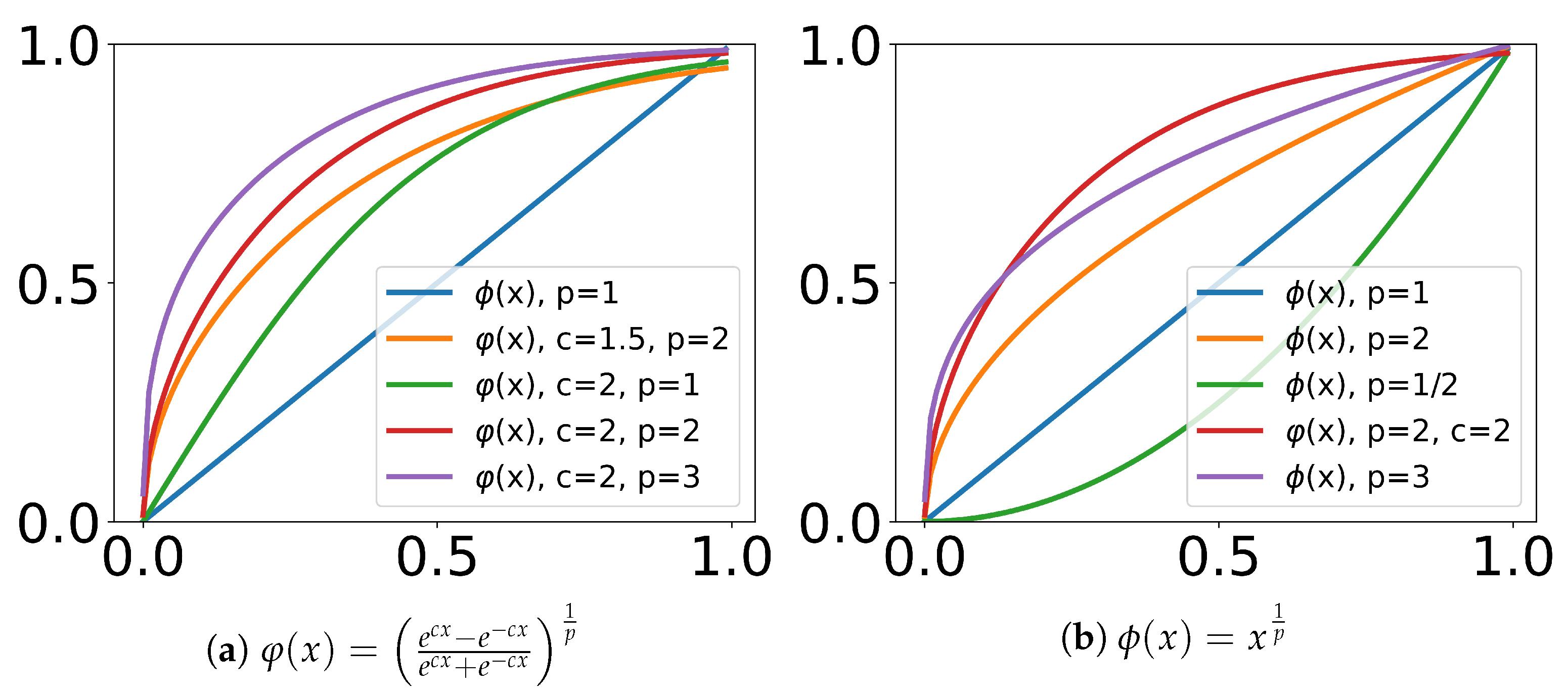
As can be seen from Figure 2b, Gamma correction gives a greater degree of enhancement when the pixel values are small. Then, two problems typically arise with Gamma correction: not enough correction and too much correction. Over-correction (in addition to making mid-tones too light) shifts colors towards neutral grey, while under-correction (in addition to making mid-tones too dark) shifts colors towards the display primaries. Unlike Gamma correction, the nonlinear transform can take into account different regions of the image by adjusting the values of the parameters c and p to give a suitable image enhancement result. The higher the values of the parameters, the steeper the transformation curve becomes; see 
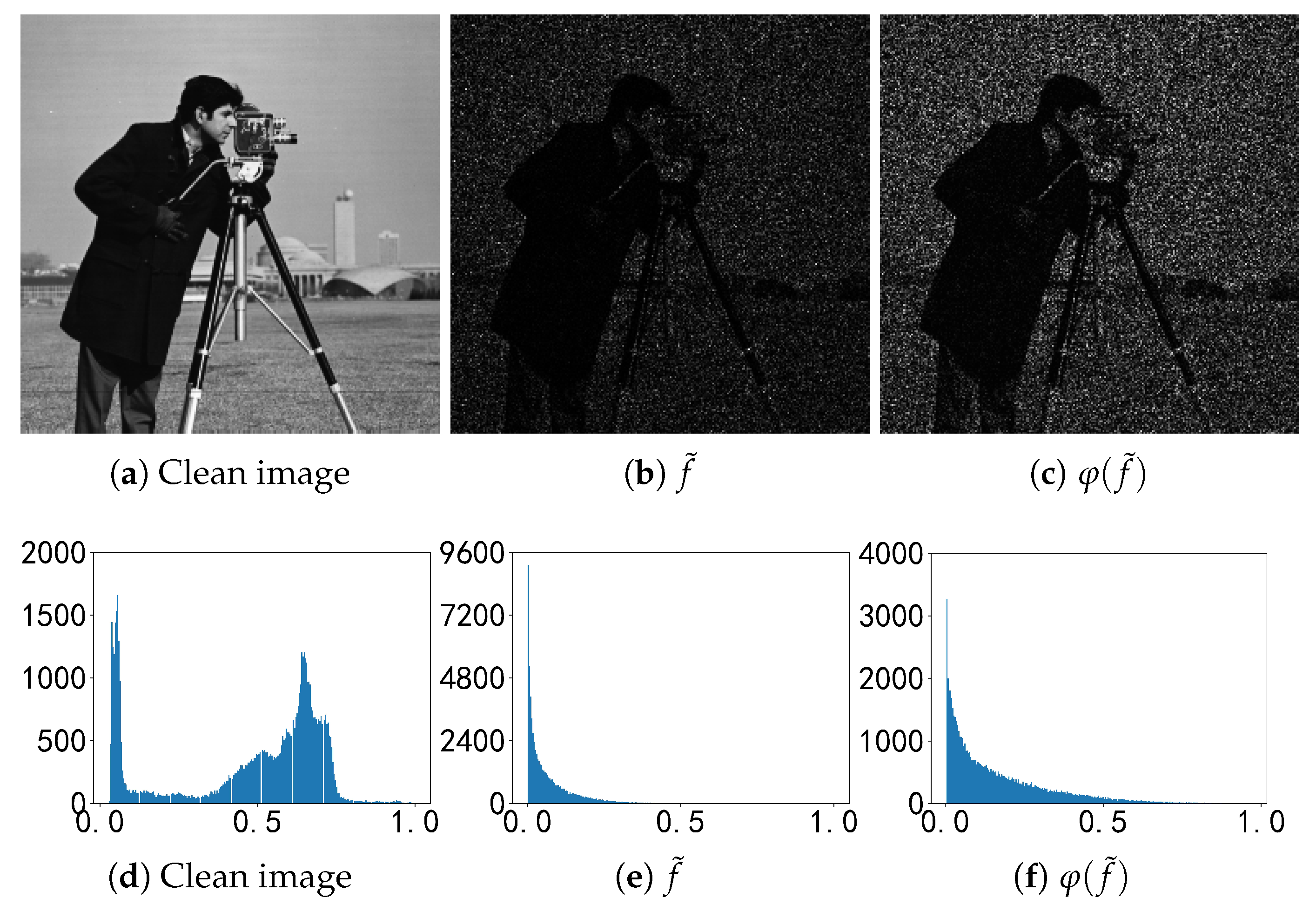
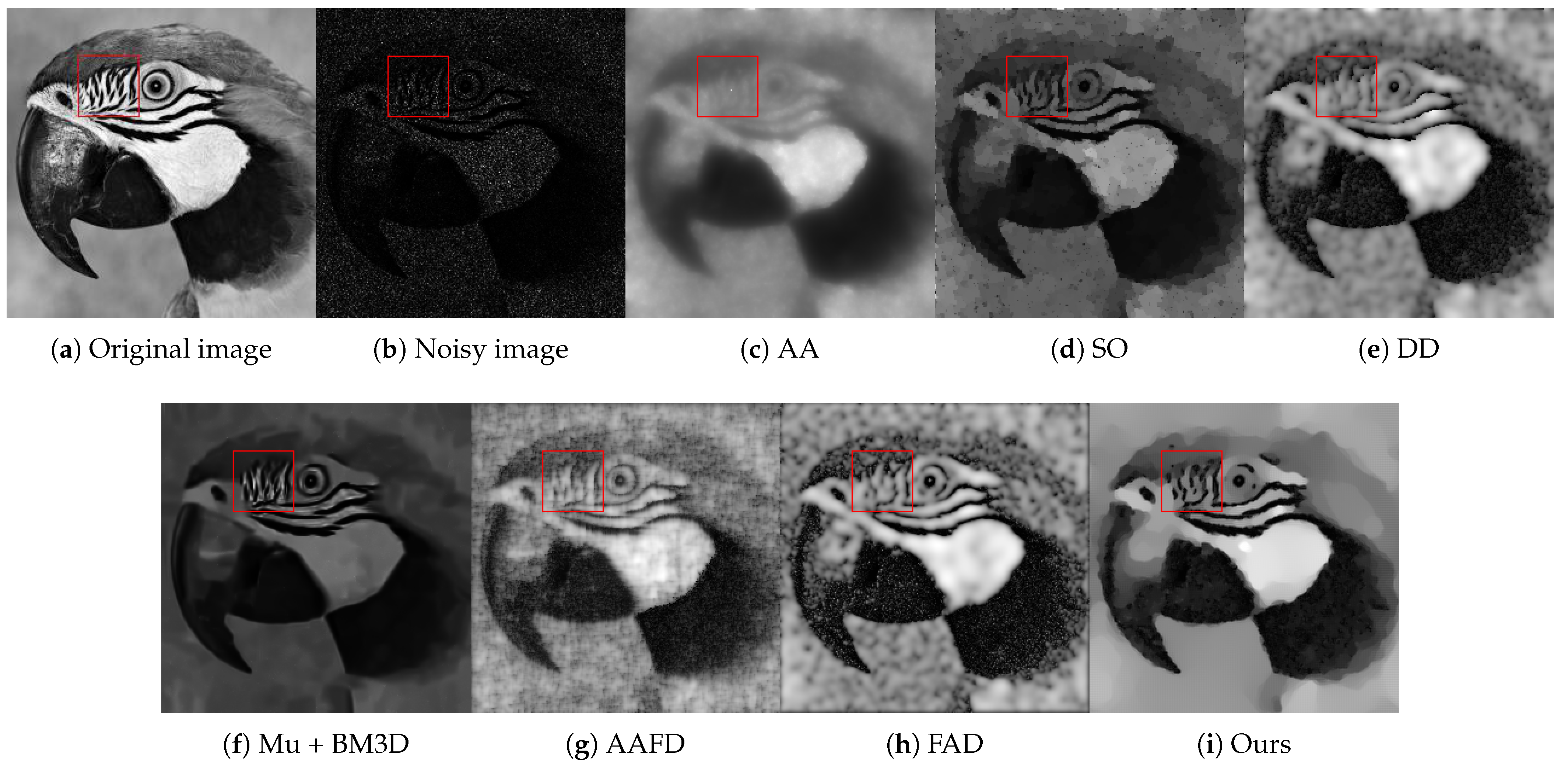
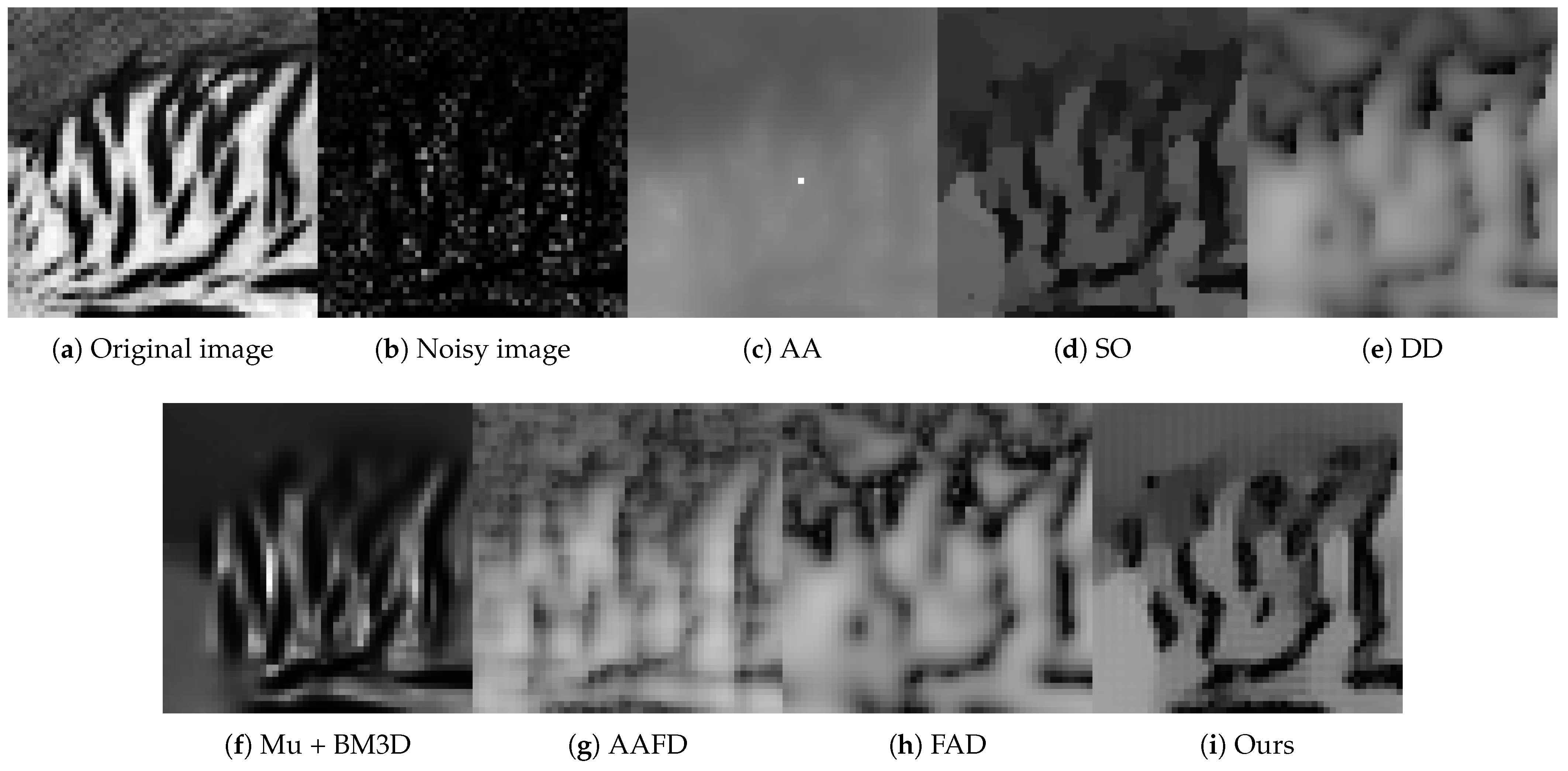
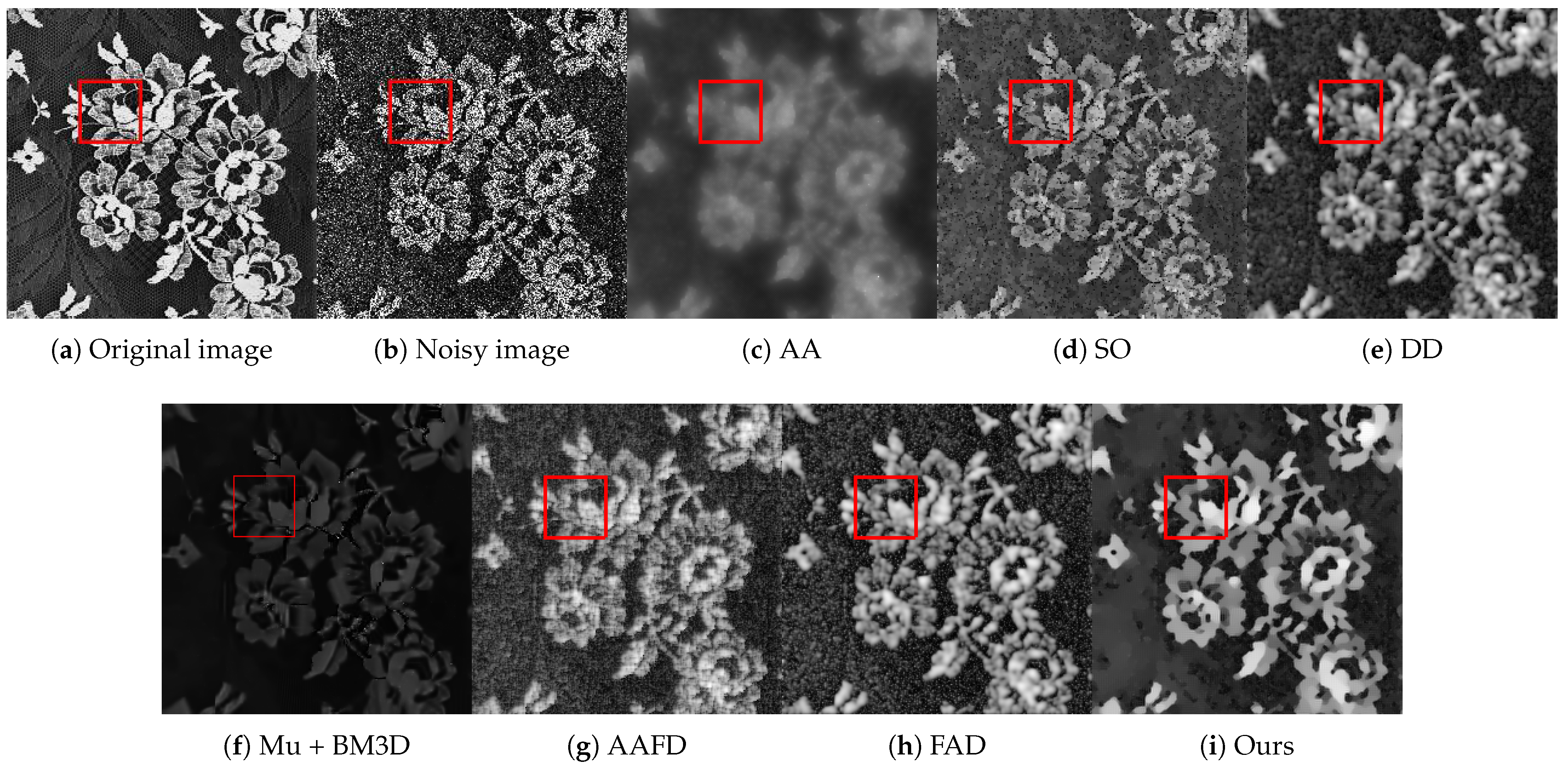
Figure 2a. To better illustrate the new degradation model, we show the original image ‘Cameraman’: the noisy image f ˜ with noise level K = 1 and the image φ ( f ˜ ) after the effect of the nonlinear transformation; see Figure 3.
It can be seen that the nonlinear transformed image shows more image details without changing the shape of the noisy image distribution. In other words, the nonlinear correction is a modification of the pixel values without changing the size, geometry, or local structure of the image.
For the inverse problem, φ ( f ˜ ) , u, and η are instances of some random variables F, U, and V. In the following, if X is a random variable, we denote g X as its density function and S as the set of the pixels of the image. Moreover, we assume that the samples of the noise on each pixel s S are mutually independent and identically distributed with density function g V .
Proposition 1.
Assume that U and V are independent random variables, with  g U  and  g V  as continuous density functions. Let us set  F = U V ; we can deduce that
sup u S ( Ω ) P ( U = u | F = φ ( f ˜ ) ) inf u S ( Ω ) Ω log   u + φ ( f ˜ ) u d x + γ 1 Ω ϕ ( u ) ,
where  γ 1  is a constant and  ϕ ( u )  is a nonnegative given function. The proof of Proposition 1 is similar to that in [12].

3.2. The Proposed Model and Its Properties

In our proposed model, the fidelity term is based on MAP estimation of the new degraded model. To better protect the image information, the regularization term is based on the L 2 -norm of TV and fractional-order bounded variation. For the fractional bounded variation, we also introduce a gray level indicator and use it as the weight of the adaptive fractional bounded variation.
Specifically, we consider the hybrid total variation regularization defined as
J ( u ) = ε 2 Ω | u | 2 d x + Ω β ( x ) | α u | d x .
Ω is a bounded open subset of R n with Lipschitz boundary and β ( x ) is a positive valued continuous function on R n . In practice, β ( x ) may be chosen as
β ( x ) = φ ( f ˜ ) max ( φ ( f ˜ ) ) q ,
where x Ω , and for the sake of simplicity, we denote f ˜ ( x ) by f ˜ . φ ( f ˜ ) = e c f ˜ e c f ˜ e c f ˜ + e c f ˜ 1 p where c and q are constants, and 0 β ( x ) 1 .
Following the fidelity terms (6) obtained from MAP estimation, we propose the following multiplicative denoising model:
min { u B V α ( Ω ) L 2 ( Ω ) } E ( u ) : = ε 2 Ω | u | 2 d x + Ω β ( x ) | α u | d x + λ Ω log   u + φ ( f ˜ ) u d x ,
where λ is a positive regularization parameter controlling the balance between the two terms in the objective function. In order to present the character of the proposed fractional method, we recall the total α -order variation and bounded β -total variation introduced in [25,37].
We first review the definitions and simple properties of a fractional-order derivative. Currently, the formula derived from the GL definition is used to calculate fractional derivatives numerically. In this paper, we use the algorithm based on fractional Fourier transform (FrFT) theory to solve the model in the frequency domain.
Definition 1
(Grünwald–Letnikov derivative). Assume α is a positive real number and  0 n 1 α n , where n is an integer.  v ( x )  is a function where  x [ a , b ] ; then
a G L D x α v ( x ) = lim h 0   h α j = 0 [ ( x a ) / h ] ( 1 ) j C j α v ( x j h )
is the left-sided Grünwald–Letnikov derivative of  v ( x ) , where  [ θ ]  is the integer such that  θ 1 < [ θ ] θ , and  C j α = Γ ( α + 1 ) / [ Γ ( j + 1 ) Γ ( α j + 1 ) ]  denotes the generalized binomial coefficient. Similarly, the right-sided Grünwald–Letnikov derivative is defined as
x G L D b α v ( x ) = lim h 0   h α j = 0 [ ( b x ) / h ] ( 1 ) j C j α v ( x + j h ) .
Definition 2
(See [37]). We assume  u L 1 ( Ω )  to be in  β BV , if u has bounded total variation, i.e.,
sup ϕ Φ β Ω u div ϕ d x < ,
where  Φ β = : { ϕ C 0 l ( Ω , R n ) , | ϕ ( x ) | β ( x ) , x Ω } .
If u L 1 ( Ω ) has bounded α -total variation in Ω , there is a Radon vector measure u on Ω such that
Ω β ( x ) | D u | = : sup ϕ Φ β Ω u div ϕ d x .
Definition 3
(bounded β - T V α ). The bounded total α-order variation of u is defined by
β - T V α ( u ) : = sup ϕ Φ β Ω u d i v α ϕ d x ,
where  Φ β  denotes the space of special test functions  Φ β : = { ϕ C 0 l ( Ω , R n ) , | ϕ ( x ) | β ( x ) , x Ω } , and  | ϕ | = i = 1 d ϕ i 2 .  d i v α ϕ = i = 1 d α ϕ i x i α  and  α ϕ i x i α  denotes a fractional α-order derivative  D [ a , b ] α ϕ i  of  ϕ i  along the  x i  direction.
Based on the bounded variation (BV) seminorm, the β - B V α norm is defined by
u B V α = u L 1 + β - T V α ( u ) ,
and furthermore, the space of functions of B V α on Ω can be defined by
B V α ( Ω ) : = { u L 1 ( Ω ) | β - T V α ( Ω ) < } .
Remark 1.
The space  B V α ( Ω )  is a Banach space.
Proposition 2.
The functional  β - T V α ( u )  is convex.
Proposition 3
(Lower semicontinuity). Assuming that Ω is bounded and with a Lipschitz boundary,  u j B V α ( Ω )  and  u j u  in  L 1 ( Ω ) . Then, there exists a minimum value u, and
Ω β ( x ) D α u lim inf j   Ω β ( x ) D α u j .
Proposition 4
(A weak * topology). B V α ( Ω )  is a Banach space endowed with the norm  u B V α = u L 1 + Ω D α u . We will not use this topology, which possesses no good compactness properties. Classically, in  B V α ( Ω )  one works with the  B V α w *  topology; we have  u j u  in  L 1 ( Ω ) , and for all ϕ in  C 0 ( Ω ) N , then  Ω ϕ D α u j Ω ϕ D α u .
Proposition 5
(Compactness). Suppose that the sequence  { u K } K R  is bounded in B V α ( Ω ) . Then, there exist a subsequence  u j k  and u in  B V α ( Ω )  such that  u j k  weakly converges to u in  B V α ( Ω ) .
Theorem 1
(Existence). The functional  E ( u ) : B V α ( Ω ) R  has a minimum.
Proof. 
B V α ( Ω ) is a Banach space, E ( u ) is weak sequentially lower semicontinuous on B V α ( Ω ) , and B V α ( Ω ) is weak sequentially compact for the result of Proposition 5. With the Prop. 38.12(d) in [38], we prove that the functional E ( u ) has a minimum.    □
Proposition 6.
The functional  E ( u )  has a unique minimizer in  B V α ( Ω )  when  0 < u < 2 φ ( f ˜ ) .
Proof. 
For g ( t ) = log   t + φ ( f ˜ ) t , we have g ( t ) = 1 t φ ( f ˜ ) t 2 = t φ ( f ˜ ) t 2 and g ( t ) = 1 t 2 + 2 φ ( f ˜ ) t 3 = 2 φ ( f ˜ ) t t 3 . It can be obtained that g ( t ) is strictly convex if 0 < t < 2 φ ( f ˜ ) . Furthermore, since β - T V α ( u ) is convex, we can deduce that E ( u ) has a unique minimizer in B V α ( Ω ) .    □

3.3. Similarity Measure

Since multiplicative noise has unfavorable properties, a new similarity measure is deduced consisting of a probability density function specially chosen for this type of noise in [39], and all random variables are supposed to be real-valued, continuous, and defined on a fixed probability space ( Ω , F , g ) .
Proposition 7.
Assuming that the distribution of  U i  is unknown and the Gamma noise  V i  is distributed with  p η ( v ; θ , K ) = K K Γ ( K ) v K 1 e K v 1 R > 0 ( v ) , then we have the similarity measure function
s D D T ( φ ( f ˜ 1 ) , φ ( f ˜ 2 ) ) = 0 g F | U φ ( f ˜ 1 ) | u g F | U φ ( f ˜ 2 ) | u d u = 0 1 u 2 g V 1 φ ( f ˜ 1 ) u g V 2 φ ( f ˜ 2 ) u d u = P φ ( f ˜ 2 ) V 1 φ ( f ˜ 1 ) V 2 ( 0 ) ,
where  s D D T  is symmetric and not bounded from above. Specifically,  s D D T ( f , f ) = 1 f P V 1 V 2 ( 0 )  for all  f = f 1 = f 2 .
The proof of Proposition 7 is is similar to that in [39].
Proposition 8.
With the definitions of the similarity measure function  s D D T  and Gamma function, we have
s D D T ( φ ( f ˜ 1 ) , φ ( f ˜ 2 ) ) = K Γ ( 2 K 1 ) Γ ( K ) 2 ( φ ( f ˜ 1 ) φ ( f ˜ 2 ) ) K 1 ( φ ( f ˜ 1 ) + φ ( f ˜ 2 ) ) 2 K 1 = K Γ ( 2 K 1 ) Γ ( K ) 2 1 φ ( f ˜ 1 ) + φ ( f ˜ 2 ) 1 ( 2 + φ ( f ˜ 2 ) φ ( f ˜ 1 ) + φ ( f ˜ 1 ) φ ( f ˜ 2 ) ) L 1 .
Proof. 
With the Gamma noise distribution p η ( v ; θ , K ) = K K Γ ( K ) v K 1 e K v 1 R > 0 ( v ) , we obtain that
s D D T ( φ ( f ˜ 1 ) , φ ( f ˜ 2 ) ) = 0 1 u 2 g V 1 φ ( f ˜ 1 ) u g V 2 φ ( f ˜ 2 ) u d u = L 2 L Γ ( L ) 2 ( φ ( f ˜ 1 ) φ ( f ˜ 2 ) ) L 1 · 0 1 u 2 L exp L φ ( f ˜ 1 ) + φ ( f ˜ 2 ) u d u .
By the definition of the Gamma function [40], note the following equality:
0 A x n exp B x d x = A B 1 n Γ ( n 1 ) .
Hence, we finally obtain
s D D T ( φ ( f ˜ 1 ) , φ ( f ˜ 2 ) ) = K Γ ( 2 K 1 ) Γ ( K ) 2 ( φ ( f ˜ 1 ) φ ( f ˜ 2 ) ) K 1 ( φ ( f ˜ 1 ) + φ ( f ˜ 2 ) ) 2 K 1 = K Γ ( 2 K 1 ) Γ ( K ) 2 1 φ ( f ˜ 1 ) + φ ( f ˜ 2 ) 1 2 + φ ( f ˜ 2 ) φ ( f ˜ 1 ) + φ ( f ˜ 1 ) φ ( f ˜ 2 ) L 1 .
   □
For the similarity measure function s D D T ( φ ( f ˜ 1 ) , φ ( f ˜ 2 ) ) , one may expect for a fixed φ ( f ˜ 1 ) that this function would reach its maximum value if φ ( f ˜ 1 ) = φ ( f ˜ 2 ) . However, for L > 1 and a known φ ( f ˜ 1 ) , the similarity measure function reaches its maximum value for φ ( f ˜ 2 ) = L 1 L φ ( f ˜ 1 ) . We assume that φ ( f ˜ 2 ) u , then measure the similarity of u and φ ( f ˜ 1 ) . If L , φ ( f 1 ˜ ) is a known noise-free image with enhancement, and u φ ( f 1 ˜ ) . This means that the role of the proposed model changes from two tasks, denoising and enhancement, to enhancement of the image only. If L is small, we find that s D D T ( φ ( f ˜ 1 ) , φ ( f ˜ 2 ) ) = 1 φ ( f ˜ 1 ) + φ ( f ˜ 2 ) for the special case L = 1 . Then, φ ( f ˜ 2 ) should be small, and denoising needs to be made the top priority. In this case, u and φ ( f ˜ 1 ) should not be too close to each other, and the weight of the regularization term in the model should be increased by adjusting the parameter.

3.4. Bias Correction

In [13], Dong and Zeng found that the AA model produces an image pixel value offset after a theoretical analysis, so a bias correction for the AA-based model is necessary. In addition, they add a new quadratic term to the AA model and reduce the influences from the bias by keeping the restored image in the same scale as the degraded image f by preserving the mean, i.e., m Ω ( u * ) = m Ω ( f ) with u * as a solution. However, this strategy is not effective enough to deal with the high dynamic intensity range of SAR images, which makes noise removal and local detail enhancement difficult. In this section, we find that the new degraded model (8) is useful for reducing the influences from the bias through theoretical analysis similar to that in [41].
Proposition 9.
Suppose that  φ ( f ˜ ) = u * η , and  inf Ω   u * > 0 . Let  u *  be a solution of (6); then we have the solution  u *  satisfying
u S ( Ω ) 1 φ ( f ˜ ) d x u S ( Ω ) 1 u * d x .
Proof. 
We define a function as follows:
e ( t ) : = Ω log ( u * + t ) + φ ( f ˜ ) u * + t d x + λ Ω D ( u + t ) ,
where t ( inf Ω   u * , + ) . Since t = 0 is a local minimizer of e ( t ) , we have e ( t ) = 0 , which leads to
Ω 1 u * φ ( f ˜ ) ( u * ) 2 d x = 0 .
Then we have
Ω 1 u * d x = Ω φ ( f ˜ ) ( u * ) 2 d x .
According to H ¨ older’s inequality and the nonnegativity of u * and φ ( f ˜ ) , we obtain
Ω φ ( f ˜ ) ( u * ) 2 d x · Ω 1 φ ( f ˜ ) d x Ω 1 u * d x 2 .
Combining both, we then have
Ω 1 φ ( f ˜ ) d x Ω 1 u * d x .
   □
Due to the new degraded model (5), f ˜ is normalized to deal with the high dynamic range problem, and φ ( f ˜ ) is adjustable with the parameter c and p. If c 1 > c 2 and p 1 > p 2 , then φ 1 ( f ˜ ) > φ 2 ( f ˜ ) . Thus, the nonlinear transformation function φ ( f ˜ ) makes it possible to give a proper bias correction on (8). With the new degraded model (5), we can not only enhance the local contrast of the restoring images but also give a satisfactory bias correction by selecting the best parameters c and p. Because better peak signal-to-noise ratio (PSNR) results can usually be obtained with a small bias, complete elimination of bias is not necessary.

4. SAV Algorithm for Solving the Proposed Variational Model

There are a number of numerical algorithms available for solving the variational model (7), such as the Split–Bregman algorithm [42], primal-dual algorithm in [43,44,45], and alternating direction method [46,47] which are widely used to solve L 1 regularization. However, these optimization algorithms are mainly used to deal with linear models, and their convergence is also based on the corresponding linear models. In order to solve the nonlinear model, Shen et al. [48] extended the IEQ to the scalar auxiliary variable (SAV), resulting in more robust schemes with less restrictions on the energy functionals. In this paper, we solve problem (7) by adopting the SAV approach.
The SAV approach is used to solve the minimization problem for a free energy functional E ( u ) . The problem can be modeled by partial differential equations having the form of gradient flows in L 2 , which can be written as
u t = μ ,
where μ = E u denotes the variational derivative.
The typical free energy functional E ( u ) usually contains a quadratic term, which can be written as
E ( u ) = Ω ε 2 | u | 2 + F ( u ) d x + C 0 ,
where F ( u ) is a nonlinear term. In order to employ the SAV approach, E ( u ) should be bounded from below [49], i.e., there always exists a positive constant C 0 such that E ( u ) + C 0 > 0 . Therefore, we modify E by adding a positive constant C 0 to E without altering the gradient flow.
Consider the proposed free energy functional E 1 ( u ) = Ω F ( u ) d x + C 0 , where
F ( u ) = Ω β ( x ) | α u | d x + λ Ω log   u + φ ( f ˜ ) u d x .
Then, the corresponding gradient flow in L 2 is as follows:
u t = μ , μ = E / u = ε Δ u + F ( u ) .
By introducing a scalar auxiliary variable r = E 1 ( u ) , the problem (9) can be equivalently rewritten as
u t = μ , μ = ε Δ u + r E 1 ( u ) F ( u ) , d r d t = 1 2 E 1 ( u ) Ω F ( u ) u t d x .
Then, a first-order SAV scheme with explicit treatment for problem (12) is as follows:
u n + 1 u n δ t = μ n + 1 ,
μ = ε Δ u n + 1 + r ¯ n + 1 E 1 ( u n ) F ( u n ) ,
r ¯ n + 1 r n δ t = 1 2 E 1 ( u n ) Ω F ( u n ) u n + 1 u n δ t d x .
We used the same strategy as in [49], updating the variable r n + 1 via r n + 1 = E 1 ( u n ) . Next, we will analyze the stability property of the scheme in the following theorem.
Theorem 2.
The scheme (13)–(15) is unconditionally stable in the sense that the following discrete energy law holds
ε 2 2 u n + 1 0 2 + | r n + 1 | 2 ε 2 2 u n 0 2 + | r n | δ t μ 0 2 ,
where  r n = E 1 ( u n ) .
In addition to the unconditional stability, the scheme (13)–(15) can be efficiently implemented. Firstly, we eliminate μ n + 1 and r ¯ n + 1 from (13)–(15) to obtain
u n + 1 u n δ t = ε Δ u n + 1 F ( u n ) E 1 ( u n ) r n + Ω F 1 ( u n ) 2 E 1 ( u n ) ( u n + 1 u n ) d x .
Let
b n = F ( u n ) E 1 ( u n ) ,
then the above equation can be written as
( I δ t ε Δ ) u n + 1 + δ t 2 b n ( b n , u n + 1 ) = u n δ t r n b n + δ t 2 ( b n , u n ) b n = g n .
To determine ( b n , u n + 1 ) from the above equation, we multiply (16) with ( I ε δ t Δ ) 1 and denote A = I ε δ t Δ . Taking the inner product with b n , we then obtain
( b n , u n + 1 ) + δ t 2 γ n ( b n , u n + 1 ) = ( b n , A 1 g n ) ,
where γ n = ( b n , A 1 b n ) . Since Δ is a positive operator, we then have A = I ε δ t Δ 0 and γ n = ( b n , A 1 b n ) 0 . With the equation above, we deduce that
( b n , u n + 1 ) = ( b n , A 1 g n ) 1 + δ t γ n / 2 .
(i)
Calculation of b n and g n : solving the elliptic problem (16), we can also obtain γ n = ( b n , A 1 b n ) .
(ii)
Evaluation of ( b n , u n + 1 ) using (17).
(iii)
With ( b n , u n + 1 ) known, we can Calculate u n + 1 from (16) as
u n + 1 = δ t 2 A 1 b n ( b n , u n + 1 ) + A 1 g n .
The adaptive time step technique allows us to reduce the computation time compared to keeping the time step constant [50,51]. In order to reduce the computation time, we adopt the same adaptive time stepping strategy for our provably stable scheme. This adaptive time step strategy is applied in Algorithm 1. The local error of a numerical method with order p is modeled as t o l = e k = C ( τ k ) p + 1 , where τ denotes the time step size, C is a constant, and t o l is a reference tolerance. Here, we set t o l 0.7 . Then, we use to update the time step size
F ( e k , τ k ) = ρ t o l e k 1 2 τ k ,
where ρ is a default coefficient, and we chose ρ = 0.8 . In addition, the minimum and maximum time steps are set as τ m i n = 10 4 and τ m a x = 10 1 .
Algorithm 1 SAV algorithm to solve the proposed model.
Input: f, λ , p, q, c, r, α , τ .
Initialize:  f ˜ = f max ( f ) , u i , j 0 = φ r ( f ˜ ) max   φ r ( f ˜ ) , φ ( f ˜ ) .
Calculation: compute u n + 1 by the first-order SAV scheme with τ n .
Update: e n + 1 = E ( u n ) E ( u n + 1 ) E ( u n + 1 ) .
if  e n + 1 > t o l  then
   recalculate time step τ n = max { τ m i n , min { F ( e n + 1 , τ n ) } } and go to step 3;
else
   update τ n + 1 = max { τ m i n , min { F ( e n + 1 , τ n ) } } . Stop or set n = n + 1 and go to step 3;
end if
return  I = u max ( u ) × 255 .

Computation of the Algorithm in the Frequency Domain

Fractional-order derivatives in the frequency domain are easy to calculate numerically due to the fast discrete Fourier transform. Therefore, we use the Fourier transform to define the fractional-order derivative in this paper. The SAV algorithm is based on 2D DFT to solve the proposed model. It is one important aspect of the algorithm that it considers the input image as a periodic image, which is equivalent to imposing a period boundary condition on the proposed model. However, discontinuities across the image borders are unavoidable in practice. In this paper, we use a similar algorithm as in [52] by extending the image symmetrically about its borders in order to reduce the discontinuities across the image borders.
Using the two-dimensional (2D) discrete Fourier transform, for any function g ( x , y ) L 2 ( R 2 ) , we obtain
g ^ ( ω 1 , ω 2 ) = R 2 g ( x , y ) exp ( j ( ω 1 x + ω 2 y ) ) d x d y
and the fractional order derivatives are
D x α g ( x , y ) = 1 2 π R 2 exp ( j ( ω 1 x + ω 2 y ) ) ( j ω 1 ) α g ^ ( ω 1 , ω 2 ) d ω 1 d ω 2 , D x α g ( x , y ) = 1 2 π R 2 exp ( j ( ω 1 x + ω 2 y ) ) ( j ω 2 ) α g ^ ( ω 1 , ω 2 ) d ω 1 d ω 2 ,
where ( x , y ) R 2 .
In the actual numerical implementation, we use the 2D discrete Fourier transform to calculate the fractional-order derivative. It is an important aspect of the algorithm that it treats the input image as a periodic image. We sample the original continuous image by the N × N uniform grid and obtain u ( x , y ) = u ( x Δ x , y Δ y ) for { x , y 0 , 1 , , N 1 } , where the grid size Δ x = Δ y = 1 .
The 2D discrete Fourier transform of u ( x , y ) is
u ^ ( ω 1 , ω 2 ) = 1 m x , y = 0 m 1 u ( x , y ) exp ( j 2 π ( ω 1 x + ω 2 y ) / m ) ,
where ω 1 { 0 , 1 , , N 1 } and ω 2 { 0 , 1 , , N 1 } are the frequencies which correspond to x and y.
With the translation property of the 2D DFT
u ( x x 0 , y y 0 ) exp ( j 2 π ( ω 1 x 0 + ω 2 y 0 ) / m ) u ^ ( ω 1 , ω 2 ) ,
the first-order partial difference in the frequency domain can be obtained as
u ( x , y ) u ( x 1 , y ) ( 1 exp ( j 2 π ω 1 / m ) ) α u ^ ( ω 1 , ω 2 ) .
Thus, the fractional-order partial difference in the frequency domain is defined as
D x α u ( 1 exp ( j 2 π ω 1 / m ) ) α u ^ ( ω 1 , ω 2 ) .
Then, we use the central difference scheme in [24] to compute the fractional-order difference, which can be defined as
D ˜ x α u = F 1 ( ( 1 exp ( j 2 π ω 1 / m ) ) α × exp ( j π ω 1 / m ) ) F ( u ) , D ˜ y α u = F 1 ( ( 1 exp ( j 2 π ω 2 / m ) ) α × exp ( j π ω 2 / m ) ) F ( u ) ,
where the notation F denotes the 2D DFT operator and the notation F 1 denotes the 2D inverse discrete Fourier transform (IDFT) operator. To simplify, let K be a purely diagonal operator defined by
K = diag ( ( 1 exp ( j 2 π ω 2 / m ) ) α × exp ( j π ω 2 / m ) ) .
Then, we obtain
D ˜ x α = F 1 K F
and
D ˜ x α * = ( F 1 K F ) * = F 1 K * F ,
where D ˜ x α * is the adjoint of D ˜ x α and ( F 1 ) * = F . Similarly, D ˜ y α * can also be obtained. Since K * is the complex conjugation of K, we have
D ˜ x α * = F 1 ( c o n j ( ( 1 exp ( j 2 π ω 1 / m ) ) α × exp ( j π ω 1 / m ) ) ) F ( u ) , D ˜ y α * = F 1 ( c o n j ( ( 1 exp ( j 2 π ω 1 / m ) ) α × exp ( j π ω 2 / m ) ) ) F ( u ) ,
where conj ( · ) is the complex conjugation.
According to the problem (11), we compute F ( u n ) by
F ( u n ) = β ( x ) D ˜ x α * D ˜ x α u n | α u n | 2 + ε 1 + β ( x ) D ˜ y α * D ˜ y α u n | α u n | 2 + ε 1 + λ u φ ( f ˜ ) u 2 ,
where ε 1 is a sufficiently small positive parameter.

5. Numerical Experiments

In this section, we demonstrated the practical performance of the proposed model solved by the SAV algorithm. To illustrate the performance of our method, the results are compared with those of the AA model [12], the SO model [13], the DD model [20], the MuLoG + BM3D model [53], FAD model [27], and AAFD model [26]. We test the models on four high-resolution images, as shown in Figure 4.
Each image is corrupted by multiplicative noise with K = 1 , K = 4 , and K = 10 . For the original image u 0 , the quality of the restored images is measured in terms of peak signal-to-noise ratio (PSNR),
P S N R = 10   log 10   M N | max   u 0 min   u 0 . | u u 0 L 2 2 ,
and mean absolute deviation error MAE,
M A E = u u 0 L 1 M N ,
where | max   u 0 min   u 0 | gives the gray-scale range of the original image, and M and N are the size of the image. Because the structural similarity measure (SSIM) is sensitive to structural content and measures the similarity between an original image u 0 and its denoised result u, it is also used in this paper.
Since SAR images are captured at different times, in different weather, and by different amounts of scattering, the captured images always have more noise in them, which is known as speckle and multiplicative noise in nature. Due to the corruption of multiplicative speckle noise, SAR images are always dark and have poor contrast. Figure 5 shows the visualization of real SAR data in [ 0 , 1 ] , and the corresponding colorbar is also depicted. To illustrate the denoising and enhancement capabilities of the models mentioned above, we test the models on the three real SAR images.

Numerical Implementations

We compare our method and competing approaches on four high-resolution images, as shown in Figure 4.
The parameters and stopping criterion of all algorithms are tweaked mutually to achieve the maximum PSNR or the best MAE and SSIM, and the choices of the parameters are tabulated in Table 1. For the MuLoG + BM3D algorithm, the free parameters are set as suggested in the reference paper [53]. These images have the range [ 1 , 255 ] (we set f = max ( f , 1 ) ) ; we first consider the restoration of ‘Parrot’, which is degraded by different noise levels of K = 1 , 4 , 10 and whose degraded images are normalized into the range [ 0 , 1 ] .
For a fair comparison, we present the PSNR, MAE, SSIM, and CPU Times values of the restoration results in Table 2 and Table 3. These tables show that the proposed model solved by the SAV algorithm achieves higher PSNR and SSIM values. Furthermore, the numerical experiments of multiplicative noise removal and contrast enhancement for the test images are depicted in Figure 6, Figure 7, Figure 8 and Figure 9. In the case of strong noise ( K = 1 ), the denoised results of the AA algorithm, the SO algorithm, and the DD algorithm show that much more noise still remains. The restored images of the AAFD algorithm and FAD algorithm show that they can remove multiplicative noise more effectively than the other TV-based algorithms do. However, the AAFD algorithm and FAD algorithm have some difficulties in bringing back some isolated points in the range of the image and keeping image details simultaneously. In Figure 6, Figure 7, Figure 8 and Figure 9, the restored images obtained by the MuLoG + BM3D algorithm tend to be over-smoothed, which makes the texture details disappear. Moreover, when the noisy image is normalized, the overall image is dark, the artificial effect is caused by stacking the image blocks [54], and the value of PSNR is not satisfactory. For these reasons, the MuLoG + BM3D algorithm may not be suitable for removing noise and enhancing the contrast of real SAR images.
In contrast, our model solved by the SAV algorithm can both preserve the texture and enhance the contrast successfully. To give a visual impression of the comparison between these different models, we also depict the respective results of these images, where we show only a fraction of the restored images, as shown in Figure 7 and Figure 9. Since the difference between the restored image and the original clean image helps to judge the ability to remove noise, we chose close-ups of the head region of Parrot and the texture region of D42. Comparing the textures surrounding the eye and the background of the Parrot, we can clearly see that our model suppresses noise successfully while preserving significantly more details. The zoomed version of the image D42 also implies that our model has the advantage of keeping the features, especially when recovering the images corrupted by strong noises. In addition, it is easy to find that our proposed model can efficiently keep edges and preserve details. In this section, we also test the four images for noise density with K = 4 , 10 , then the same conclusion about restoration capability can be obtained from Table 2. This still shows that our proposed model can achieve good restoration results at different noise levels.
Since the model we solved with the SAV algorithm performs well in image denoising and contrast enhancement with strong multiplicative noise levels, we tried to use this model to solve the problem of denoising and image information enhancement of SAR images. Unlike optical images, SAR images have a large dynamic range of intensity and rich texture information. The local information is too important to be smoothed, which highlights the significance of simultaneously removing multiplicative noise and enhancing the texture contrast of the restored image within the appropriate pixel range. In Figure 10, Figure 11 and Figure 12, we give the restoration results for SAR images and find that the DD model and the FAD model perform slightly better than the other models. However, the local details of the restoration results obtained by the DD model are blurred, and the restoration results obtained by the FAD model have residual speckle noise, while our model solved by the SAV algorithm retains more topographic information and gives more satisfying edges. The histogram of each restoration image shows the distribution of pixel values; our method also performs best both visually and quantitatively. In Table 2, we list the SSIM (structural similarity index) values and the CPU times. In contrast to the results for the AA, SO, DD, MuLoG + BM3D, AAFD, and FAD models, our method solved by the SAV algorithm provides satisfactory results with high SSIM (structural similarity index) values. In Figure 13, the plots of energy are monotonically decreasing; our model solved by the SAV algorithm converges to a minimum value.

6. Conclusions

In this paper, we study the restoration and enhancement of texture information of SAR images under multiplicative noise corruption. To address the problems that SAR images have a larger range of pixel values and that traditional denoising methods are prone to step effects and degradation of image contrast, we propose a fractional-order variation model based on the nonlinear transformation. Specifically, a degradation model is proposed by using a nonlinear transformation to adjust the intensity of image pixel values, and the fidelity term of the variational model is constructed by maximum a posteriori (MAP) estimation. The fidelity term obtained is useful for reducing the influences from the bias through theoretical analysis. To overcome the staircase effect often produced by existing denoising algorithms, we introduce a gray level indicator in the regularization term. In addition, considering the characteristics of SAR images with large pixel values and no uniform range, the normalization method is introduced to fix the images in the specified range to avoid the problem of missing SAR image information caused by the truncation function. Under certain conditions, we prove the existence of a minimizer and we show the capability of our model on some numerical examples.

Author Contributions

Conceptualization, Y.Z. and Y.L.; methodology, all authors; software, Y.Z. and Y.L.; validation, Y.Z., Y.L., and Z.G.; formal analysis, Y.Z. and Y.L.; investigation, Y.Z. and Y.L.; resources, Y.Z. and Z.G.; data curation, Y.Z. and Y.L.; writing—original draft preparation, Y.Z. and Y.L.; writing—review and editing, Y.Z., B.W. and D.Z.; visualization, Y.Z. and Z.G.; supervision, Y.Z. and Y.L.; project administration, Z.G. and D.Z.; funding acquisition, D.Z., Z.G. and Y.L. All authors have read and agreed to the published version of the manuscript.

Funding

This work was partially supported by the National Natural Science Foundation of China (12271130, 11971131, U21B2075, 12171123, 11871133), Natural Science Foundation of Heilongjiang Province (ZD2022A001), Basic and Applied Basic Research Foundation of Guangdong Province (2020B1515310006), Funding Heilongjiang Provincial Postdoctoral Science Foundation (LBH-Z21157), and Fundamental Research Funds for the Central Universities (2022FRFK060014, 2022FRFK060020, 2022FRFK060031, HIT.NSRIF202202), China Society of Industrial and Applied Mathematics Young Women Applied Mathematics Support Research Project.

Data Availability Statement

The data used to support the findings of this study are available from the corresponding author upon request.

Conflicts of Interest

The authors declare that they have no conflict of interest.

References

  1. Baraha, S.; Sahoo, A.; Modalavalasa, S. A systematic review on recent developments in nonlocal and variational methods for SAR image despeckling. Signal Process. 2022, 196, 108521. [Google Scholar] [CrossRef]
  2. Bailey, D.; Townsend, D.; Valk, P.; Maisey, M. Positron Emission Tomography: Basic Sciences; Springer: London, UK, 2005. [Google Scholar]
  3. Bamler, R. Principles of synthetic aperyure rader. Surv. Geophys. 2000, 21, 147–157. [Google Scholar] [CrossRef]
  4. Schmitt, J.; Xiang, S.; Yung, K. Speckle in optical coherence tomography. J. Biomed. Opt. 1999, 4, 95–105. [Google Scholar] [CrossRef]
  5. Wagner, R. Statistics of speckle in ultrasound B-scans. IEEE Trans. Sonics Ultrason. 1983, 30, 156–163. [Google Scholar] [CrossRef]
  6. Han, J.; Nam, W.; Lee, S. SAR image denoising in high dynamic range with speckle and thermal noise refinement modeling. In Proceedings of the 2022 18th IEEE International Conference on Advanced Video and Signal Based Surveillance (AVSS), Madrid, Spain, 29 November–2 December 2022; pp. 1–8. [Google Scholar]
  7. Benz, U.; Strodl, K.; Moreira, A. A comparison of several algorithms for SAR raw data compression. IEEE Trans. Geosci. Remote Sens. 1995, 33, 1266–1276. [Google Scholar] [CrossRef]
  8. Dellepiane, S.; Angiati, E. A new method for cross-normalization and multitemporal visualization of SAR images for the detection of flooded areas. IEEE Trans. Geosci. Remote Sens. 2012, 50, 2765–2779. [Google Scholar] [CrossRef]
  9. Boschetti, A.; Adami, N.; Leonardi, R.; Okuda, M. High dynamic range image tone mapping based on local histogram equalization. In Proceedings of the 2010 IEEE International Conference on Multimedia and Expo, Singapore, 19–23 July 2010; pp. 1130–1135. [Google Scholar]
  10. Ahn, H.; Keum, B.; Kim, D.; Lee, H. Adaptive local tone mapping based on retinex for high dynamic range images. In Proceedings of the 2013 IEEE International Conference on Consumer Electronics (ICCE), Las Vegas, NV, USA, 11–14 January 2013; pp. 153–156. [Google Scholar]
  11. Easton, J.; Roger, L. Digital Image Processing I; Prentice Hall Press: Hoboken, NJ, USA, 2010. [Google Scholar]
  12. Aubert, G.; Aujol, J. A variational approach to removing multiplicative noise. SIAM J. Appl. Math. 2008, 68, 925–946. [Google Scholar] [CrossRef]
  13. Dong, Y.; Zeng, T. A convex variational model for restoring blurred images with multiplicative noise. Siam J. Imaging Sci. 2013, 6, 1598–1625. [Google Scholar] [CrossRef]
  14. Zhang, J.; Chen, K.; Yu, B. An iterative Lagrange multiplier method for constrained total-variation-based image denoising. SIAM J. Numer. Anal. 2012, 50, 983–1003. [Google Scholar] [CrossRef]
  15. Wei, W.; Yao, M.; Michael, K. Color image multiplicative noise and blur removal by saturation-value total variation. Appl. Math. Model. 2021, 90, 240–264. [Google Scholar]
  16. Shi, J.; Osher, S. A nonlinear inverse scale space method for a convex multiplicative noise model. Siam J. Imaging Sci. 2008, 1, 294–321. [Google Scholar] [CrossRef]
  17. Lysaker, M.; Lundervold, A.; Tai, X. Noise removal using fourth-order partial differential equation with applications to medical magnetic resonance images in space and time. IEEE Trans. Image Process. 2003, 12, 1579–1590. [Google Scholar] [CrossRef] [PubMed]
  18. Krissian, K.; Westin, C.-F.; Kikinis, R.; Vosburgh, K.G. Oriented speckle reducing anisotropic diffusion. IEEE Trans. Image Process. 2007, 16, 1412–1424. [Google Scholar] [CrossRef] [PubMed]
  19. Yu, Y.; Acton, S. Speckle reducing anisotropic diffusion. IEEE Trans. Image Process. 2002, 11, 1260–1270. [Google Scholar]
  20. Zhou, Z.; Guo, Z.; Dong, G.; Sun, J.; Zhang, D.; Wu, B. A doubly degenerate diffusion model based on the gray level indicator for multiplicative noise removal. IEEE Trans. Image Process. 2014, 24, 249–260. [Google Scholar] [CrossRef]
  21. Majee, S.; Ray, R.; Majee, A. A gray level indicator-based regularized telegraph diffusion model: Application to image despeckling. Siam J. Imaging Sci. 2020, 13, 844–870. [Google Scholar] [CrossRef]
  22. Li, C.; He, C. Fractional-order diffusion coupled with integer-order diffusion for multiplicative noise removal. Comput. Math. Appl. 2023, 136, 34–43. [Google Scholar] [CrossRef]
  23. Bai, X.; Zhang, D.; Shi, S.; Yao, W.; Guo, Z.; Sun, J. A fractional-order telegraph diffusion model for restoring texture images with multiplicative noise. Fractal Fract. 2023, 7, 64. [Google Scholar] [CrossRef]
  24. Bai, J.; Feng, X. Fractional-order anisotropic diffusion for image denoising. IEEE Trans. Image Process. 2007, 16, 2492–2502. [Google Scholar] [CrossRef] [PubMed]
  25. Zhang, J.; Chen, K. A total fractional-order variation model for image restoration with nonhomogeneous boundary conditions and its numerical solution. Siam J. Imaging Sci. 2015, 8, 2487–2518. [Google Scholar] [CrossRef]
  26. Yao, W.; Guo, Z.; Sun, J.; Wu, B.; Gao, H. Multiplicative noise removal for texture images based on adaptive anisotropic fractional diffusion equations. Siam J. Imaging Sci. 2019, 12, 839–873. [Google Scholar] [CrossRef]
  27. Shan, X.; Sun, J.; Guo, Z.; Yao, W.; Zhou, Z. Fractional-order diffusion model for multiplicative noise removal in texture-rich images and its fast explicit diffusion solving. BIT Numer. Math. 2022, 62, 1319–1354. [Google Scholar] [CrossRef]
  28. Zhang, J.; Chen, J.; Yu, H.; Yang, D.; Xu, X.; Xing, M. Learning an SAR image despeckling model via weighted sparse representation. IEEE J. Sel. Top. Appl. Earth Obs. Remote Sens. 2021, 14, 7148–7158. [Google Scholar] [CrossRef]
  29. Chagas, E.; Frery, A.; Rosso, O.; Ramos, H. Analysis and classification of SAR textures using information theory. IEEE J. Sel. Top. Appl. Earth Obs. Remote Sens. 2020, 14, 663–675. [Google Scholar] [CrossRef]
  30. Fattal, R.; Lischinski, D.; Werman, M. Gradient domain high dynamic range compression. In Proceedings of the 29th Annual Conference on Computer Graphics and Interactive Techniques, San Antonio, TX, USA, 23–26 July 2002; pp. 249–256. [Google Scholar]
  31. Gu, B.; Li, W.; Wong, J.; Zhu, M.; Wang, M. Gradient field multi-exposure images fusion for high dynamic range image visualization. J. Vis. Commun. Image Represent. 2012, 23, 604–610. [Google Scholar] [CrossRef]
  32. Sundaram, M.; Ramar, K.; Arumugam, N.; Prabin, G. Histogram based contrast enhancement for mammogram images. In Proceedings of the International Conference on Signal Processing, Communication, Computing and Networking Technologies, Tamil Nadu, India, 21–22 July 2011; pp. 842–846. [Google Scholar]
  33. Abdullah-Al-Wadud, M.; Kabir, M.; Dewan, M.; Chae, O. A dynamic histogram equalization for image contrast enhancement. IEEE Trans. Consum. Electron. 2007, 53, 593–600. [Google Scholar] [CrossRef]
  34. Zimmermann, H. Fuzzy Set Theory—And Its Applications; Springer Science & Business Media: Berlin/Heidelberg, Germany, 2011. [Google Scholar]
  35. Kim, M.; Chung, M. Recursively separated and weighted histogram equalization for brightness preservation and contrast enhancement. IEEE Trans. Consum. Electron. 2008, 54, 1389–1397. [Google Scholar] [CrossRef]
  36. Tobias, O.; Seara, R. Image segmentation by histogram thresholding using fuzzy sets. IEEE Trans. Image Process 2002, 11, 1457–1465. [Google Scholar] [CrossRef]
  37. Chen, Y.; Rao, M. Minimization problems and associated flows related to weighted p energy and total variation. SIAM J. Math. Anal. 2003, 34, 1084–1104. [Google Scholar] [CrossRef]
  38. Zeidler, E. Nonlinear Functional Analysis and Its Applications: III: Variational Methods and Optimization; Springer Science & Business Media: Berlin/Heidelberg, Germany, 2013. [Google Scholar]
  39. Teuber, T.; Lang, A. A new similarity measure for nonlocal filtering in the presence of multiplicative noise. Comput. Stat. Data Anal. 2012, 56, 3821–3842. [Google Scholar] [CrossRef]
  40. Deledalle, C.; Denis, L.; Tupin, F. Iterative weighted maximum likelihood denoising with probabilistic patch-based weights. IEEE Trans. Image Process. 2009, 18, 2661–2672. [Google Scholar] [CrossRef] [PubMed]
  41. Chambolle, A.; Lions, P. Image recovery via total variation minimization and related problems. Numer. Math. 1997, 76, 167–188. [Google Scholar] [CrossRef]
  42. Goldstein, T.; Osher, S. The split Bregman method for L1-regularized problems. SIAM J. Imaging Sci. 2009, 2, 232–243. [Google Scholar] [CrossRef]
  43. Chan, T.; Golub, G.; Mulet, P. A nonlinear primal-dual method for total variation-based image restoration. Siam J. Sci. Comput. 1999, 20, 1964–1977. [Google Scholar] [CrossRef]
  44. Chambolle, A. An algorithm for total variation minimization and applications. J. Math. Imaging Vis. 2004, 20, 89–97. [Google Scholar]
  45. Zhu, M.; Chan, T. An efficient primal-dual hybrid gradient algorithm for total variation image restoration. UCLA Cam Rep. 2008, 34, 8–34. [Google Scholar]
  46. Boyd, S.; Parikh, N.; Chu, E.; Peleato, B.; Eckstein, J. Distributed optimization and statistical learning via the alternating direction method of multipliers. Found. Trends Mach. Learn. 2011, 3, 1–122. [Google Scholar] [CrossRef]
  47. Figueiredo, M.; Bioucas-Dias, J. Restoration of Poissonian images using alternating direction optimization. IEEE Trans. Image Process. 2010, 19, 3133–3145. [Google Scholar] [CrossRef]
  48. Shen, J.; Xu, J.; Yang, J. A new class of efficient and robust energy stable schemes for gradient flows. SIAM Rev. 2019, 61, 474–506. [Google Scholar] [CrossRef]
  49. Hou, D.; Azaiez, M.; Xu, C. A variant of scalar auxiliary variable approaches for gradient flows. J. Comput. Phys. 2019, 395, 307–332. [Google Scholar] [CrossRef]
  50. Gomez, H.; Calo, V.; Bazilevs, Y.; Hughes, T. Isogeometric analysis of the Cahn-Hilliard phase-field model. Comput. Methods Appl. Mech. Eng. 2008, 197, 49–50. [Google Scholar] [CrossRef]
  51. Einkemmer, L. An adaptive step size controller for iterative implicit methods. Appl. Numer. Math. 2018, 132, 182–204. [Google Scholar] [CrossRef]
  52. Do, M.; Vetterli, M. The finite ridgelet transform for image representation. IEEE Trans. Image Process. 2003, 12, 16–28. [Google Scholar] [CrossRef] [PubMed]
  53. Deledalle, C.; Denis, L.; Tabti, S.; Tupin, F. MuLoG, or how to apply Gaussian denoisers to multi-channel SAR speckle reduction? IEEE Trans. Image Process. 2017, 26, 4389–4403. [Google Scholar] [CrossRef] [PubMed]
  54. Liu, J.; Osher, S. Block matching local SVD operator based sparsity and TV regularization for image denoising. J. Sci. Comput. 2019, 78, 607–624. [Google Scholar] [CrossRef]
Figure 1. Original signal and noisy signal ( K = 1 ).
Fractalfract 07 00329 g001
Figure 2. Plots of two transformation functions.
Fractalfract 07 00329 g002
Figure 3. Histograms of the image Cameraman with noise level K = 1 .
Fractalfract 07 00329 g003
Figure 4. Test images.
Fractalfract 07 00329 g004
Figure 5. Test images.
Fractalfract 07 00329 g005
Figure 6. (b) Noisy: L = 1. (ci) Denoised results.
Fractalfract 07 00329 g006
Figure 7. The zoomed version of the Parrot image and its corresponding denoised results.
Fractalfract 07 00329 g007
Figure 8. (b) Noisy: L = 1. (ci) Denoised results.
Fractalfract 07 00329 g008
Figure 9. The zoomed version of the D4 image and its corresponding denoised results.
Fractalfract 07 00329 g009
Figure 10. Denoised results and the corresponding histograms.
Fractalfract 07 00329 g010
Figure 11. Denoised results and the corresponding histograms.
Fractalfract 07 00329 g011
Figure 12. Denoised results.
Fractalfract 07 00329 g012aFractalfract 07 00329 g012b
Figure 13. Plots of energy.
Fractalfract 07 00329 g013
Table 1. The parameter values for numerical experiments.
Parrot
Algorithm K = 1
AA( λ )5.40
SO( λ , α )0.24, 2.00
DD( α , β )2.06, 0.05
FAD( α , k, q)1.40, 0.05, 3.90
AAFD( α , β , r, k)0.50, 0.80, 1, 0.30 × 10 2
Ours( λ , α , c, p, q) 3.50 × 10 2 , 1.00, 2.10, 0.88, 0.25
Algorithm K = 4
AA( λ )7.10
SO( λ , α )1.05, 1.69
DD( α , β )3.00, 0.4
FAD( α , k, q)0.90, 0.05, 2.50
AAFD( α , β , r, k)0.60, 0.80, 1.3, 0.3 × 10 2
Ours( λ , α , c, p, q)0.20, 1.05, 1.50, 0.95, 0.35
Algorithm K = 10
AA( λ )13.00
SO( λ , α )2.30, 1.58
DD( α , β )2.50, 0.10
FAD( α , k, q)1.40, 0.05, 3.90
AAFD( α , β , r, k)0.50, 0.80, 1.00, 0.3 × 10 2
Ours( λ , α , c, p, q)0.34, 1.00, 1.50, 0.99, 0.45
Table 2. Comparisons of PSNR and MAE by using different denoising models.
NoiseK = 1K = 4K = 10
ImageFigure (a): Parrot
ModelsPSNRMAEPSNRMAEPSNRMAE
AA17.0824.2019.1020.0722.9311.46
SO19.8416.7923.7010.2025.778.29
DD19.3618.2121.4114.9223.3411.47
Mu + BM3D10.8362.0315.6934.7018.5124.79
AAFD19.0720.5321.4314.9922.6114.06
FAD19.3619.6121.9713.8324.0011.04
Ours20.4315.1823.7211.0225.688.74
ImageFigure (b): Cameraman
ModelsPSNRMAEPSNRMAEPSNRMAE
AA17.9122.8920.6617.1024.409.24
SO19.8919.3023.6310.8125.318.85
DD19.9817.6522.0114.2224.2310.62
Mu + BM3D16.4631.7823.7110.4324.878.17
AAFD19.8218.8822.0814.6123.5412.08
FAD19.8818.9821.9714.5524.5610.46
Ours21.4613.3723.8310.4025.768.29
ImageFigure (c): Boston
ModelsPSNRMAEPSNRMAEPSNRMAE
AA14.4038.4215.2134.8515.9731.77
SO15.2135.2717.9124.9519.3220.38
DD15.6132.2217.5225.5419.4520.10
Mu + BM3D14.1737.8015.8030.5316.4128.48
AAFD15.8731.5217.9625.1619.8419.75
FAD15.7132.6217.7424.9819.7019.54
Ours15.8731.5018.1723.8120.3318.24
ImageFigure (d): D4
ModelsPSNRMAEPSNRMAEPSNRMAE
AA12.3646.4813.6441.4416.2729.33
SO14.7837.2518.4122.6820.3717.37
DD14.8633.3817.2224.8119.5518.47
Mu + BM3D8.8568.7915.0631.9616.1927.82
AAFD15.3233.1017.5426.3620.1617.88
FAD15.2532.7317.4424.6419.7518.13
Ours15.7128.6318.4421.3820.5416.78
Table 3. Comparisons of SSIM and CPU Times by using different denoising models.
NoiseK = 1K = 4K = 10
ImageFigure (a): Parrot
ModelsSSIMTime(s)SSIMTime(s)SSIMTime(s)
AA0.4914.690.6347.960.7453.65
SO0.5911.610.738.200.7915.78
DD0.542.210.603.000.701.56
Mu + BM3D0.495.690.695.250.771.15
AAFD0.453.030.593.240.733.73
FAD0.4645.800.6035.500.6745.53
Ours0.66164.820.72256.140.79185.95
ImageFigure (b): Cameraman
ModelsSSIMTime(s)SSIMTime(s)SSIMTime(s)
AA0.5377.490.6425.270.7415.69
SO0.583.360.686.600.7413.07
DD0.552.160.590.690.610.47
Mu + BM3D0.665.990.755.290.775.30
AAFD0.423.420.495.410.572.38
FAD0.4235.790.5025.240.6420.03
Ours0.62123.140.67223.820.77183.61
ImageFigure (c): Boston
ModelsSSIMTime(s)SSIMTime(s)SSIMTime(s)
AA0.1314.220.2214.760.3220.30
SO0.369.250.5214.060.6526.03
DD0.300.950.551.390.711.10
Mu + BM3D0.275.980.325.220.354.88
AAFD0.356.600.595.680.725.07
FAD0.3044.180.5925.300.7120.13
Ours0.33319.410.60222.400.74310.08
ImageFigure (d): D4
ModelsSSIMTime(s)SSIMTime(s)SSIMTime(s)
AA0.1514.660.2314.070.4718.81
SO0.4330.750.5121.820.6933.40
DD0.380.940.561.030.671.25
Mu + BM3D0.1044.740.3845.710.4256.01
AAFD0.434.870.669.940.796.75
FAD0.4331.700.6455.870.7527.88
Ours0.42281.070.67199.180.80256.68
Disclaimer/Publisher’s Note: The statements, opinions and data contained in all publications are solely those of the individual author(s) and contributor(s) and not of MDPI and/or the editor(s). MDPI and/or the editor(s) disclaim responsibility for any injury to people or property resulting from any ideas, methods, instructions or products referred to in the content.

