Solving Some Physics Problems Involving Fractional-Order Differential Equations with the Morgan-Voyce Polynomials

Abstract

In this research, we present a new computational technique for solving some physics problems involving fractional-order differential equations including the famous Bagley–Torvik method. The model is considered one of the important models to simulate the coupled oscillator and various other applications in science and engineering. We adapt a collocation technique involving a new operational matrix that utilizes the Liouville–Caputo operator of differentiation and Morgan–Voyce polynomials, in combination with the Tau spectral method. We first present the differentiation matrix of fractional order that is used to convert the problem and its conditions into an algebraic system of equations with unknown coefficients, which are then used to find the solutions to the proposed models. An error analysis for the method is proved to verify the convergence of the acquired solutions. To test the effectiveness of the proposed technique, several examples are simulated using the presented technique and these results are compared with other techniques from the literature. In addition, the computational time is computed and tabulated to ensure the efficacy and robustness of the method. The outcomes of the numerical examples support the theoretical results and show the accuracy and applicability of the presented approach. The method is shown to give better results than the other methods using a lower number of bases and with less spent time, and helped in highlighting some of the important features of the model. The technique proves to be a valuable approach that can be extended in the future for other fractional models having real applications such as the fractional partial differential equations and fractional integro-differential equations.

1. Introduction

Fractional calculus is a branch of mathematics that deals with the study of derivatives and integrals of non-integer order. It has been around since the late 17th century when Gottfried Leibniz first proposed the concept of fractional derivatives, which has developed into a powerful tool for simulating different physical problems in many areas such as physics, chemistry, engineering, economics, and biology. The concept of fractional calculus was initially met with skepticism due to its unfamiliarity and lack of intuitive understanding. However, over time, its usefulness has been recognized and there have been various definitions and properties. These definitions vary depending on the context in which it is used, which in general have a common definition as the study of derivatives and integrals with non-integer orders. This means that instead of taking derivatives or integrals concerning a single variable (as in traditional calculus), fractional calculus allows for derivatives or integrals to be taken concerning multiple variables simultaneously. This allows for more complex phenomena such as memory effects, diffusion processes, and chaotic systems that might be difficult to solve using traditional definitions. In addition, fractional derivatives are useful in many fields such as physics, engineering, economics, and finance. For example, Zhao et al. [1] investigated the possible application of fractional definitions to simulate a class of nonlinear fractional Langevin equations with important application in fluid dynamics. In addition, Zhang et al. [2] employed an exponential Euler scheme for simulating the multi-delay Caputo–Fabrizio fractional-order differential equations with application in control theory. Additionally, other applications of fractional calculus in several branches of science and engineering include the simulation of the model of viscoelastic materials in engineering applications and financial markets in economics. They can also be used to describe chaotic systems in physics and other fields. There are various definitions of the fractional order including the Riemann–Liouville operator [3], Grünwald–Letnikov operator [4], Liouville–Caputo operator [5] and Weyl–Riesz operator [6]. Each of these definitions adheres to some advantages and disadvantageous over the other and the most widely used of these applications is the Liouville–Caputo and Riemann–Liouville operators. There is a close relationship between these two definitions since they can be converted through some regularity assumption [7]. The Liouville–Caputo fractional operator is considered a powerful tool for solving fractional differential equations (FDEs) that have been used widely for simulating different complex problems. The Liouville–Caputo fractional operator is a generalization of the classical derivative operator and can be used to solve FDEs with non-integer order derivatives. It has the advantage of simulating physical phenomena that involve memory effects or non-local interactions. In addition, it allows for more accurate solutions since it takes into account memory effects and it provides more flexibility when solving FDEs; because it can be applied to any function that can be expressed as a power expansion series. This was one of the reasons to be used for the simulation of non-integer models. For example, the definition of the Liouville–Caputo operator has been used in simulating disease models. Bonyah et al. [8] simulated the definition of the Liouville–Caputo for investigating the dynamics of the COVID-19 infection. In addition, the time-dependent influenza model has been studied in [9] to provide insight into the dynamics of such a model and to provide measure precautions to stop its spread. Additionally, Gao et al. [10] proposed a new fractional numerical differentiation formula for the Liouville–Caputo fractional derivative and tested the new formulae for multiple applications. Additionally, the constant proportional Liouville–Caputo operators were employed in [11] for simulating the dynamics of the HIV disease model to understand its dynamics and ways of spread. Han et al. identified some solutions for the variable-coefficient fractional-in-space KdV equation in [12]. Some basic therapies and applications of the fractional differential equations have been illustrated in [13] while [14,15] provided some parametric and argument variations of the operators related to fractional calculus. With the importance of such definitions, the Liouville–Caputo operator is of importance in helping to understand such behavior of complex models.

Numerical simulation using collocation and spectral methods is a powerful tool for solving complex problems in engineering and science. It is a method of approximating solutions to differential equations by utilizing computational techniques such as collocation and spectral methods. Collocation methods are used to approximate solutions to various differential equations by representing them as a linear combination of basis functions. Spectral methods are used to approximate solutions to differential equations by representing them as an infinite series of (orthogonal) polynomials. Both of these techniques have been widely used in the field of computational science, with applications ranging from fluid dynamics to quantum mechanics. Collocation techniques have been widely used for acquiring accurate results for these models using different types of bases. The main idea of this technique is that the solution to a differential equation can be represented as a linear combination of basis functions. These basis functions can be chosen from a variety of sources including polynomials or other types. For example, Izadi et al. [16] investigated the solution of the waste plastic management model in the ocean system using the Morgan–Voyce polynomials. In addition, Adel et al. [17] employed a collocation method of Genocchi polynomials for simulating the solution to the fourth-order singular singularly perturbed and Emden–Fowler problems, which have significant importance in physics. Izadi et al. [18] developed a collocation approach with a new definition of the Chelyshkov polynomials to solve the fractional delay differential equations. Additionally, El-Gamel et al. [19] adapted the Genocchi collocation method for solving a class of high-order boundary value problems. The B-spline bases have been used to simulate physical models as well as other basis functions. For example, De Boor [20] was the first to introduce the basic definitions of the B-spline basis, and then researchers have been using it to simulate real-life models. Kaur et al. [21] employed the adaptive wavelet optimized finite difference technique combined with the B-spline polynomial for the solution of random partial differential equations. Zahra et al. [22] developed a robust uniform B-spline collocation method for solving the generalized PHI-four equation. In addition, a cubic B-spline collocation algorithm has been used to solve the Newell–Whitehead–Segel type equations in [23]. Additionally, the combination of the wavelet along with other polynomials has been used in the simulation of different models [24] and Alqhtani et al. [25] simulated a high-dimensional chaotic Lorenz system using the Gegenbauer wavelet polynomials. The coefficients in the linear combination are determined by solving an optimization problem that minimizes the error between the approximate solution and the exact solution. This approach is particularly useful when dealing with boundary value problems since it allows for accurate approximations near the boundaries without having to solve for all points in between. Spectral methods on the other hand are based on the idea that solutions to differential equations can be represented as an infinite series of orthogonal polynomials. These polynomials can be chosen from a variety of sources including the Chebyshev polynomials [26] which have been used in the simulation of the fractional diffusion-wave equation by Atta et al. [27]. Another type of polynomials is the Legendre polynomials [28], which is also used for solving the linear Fredholm integro-differential equations accompanied by the Galerkin method by Fathy et al. [29]. In addition, Abdelhakem et al. [30] employed the pseudo-spectral matrices method for treating some models using the Legendre polynomials. More general orthogonal polynomials such as Hermite [31] or Laguerre polynomials [32] have also been used in practical simulations. This approach is particularly useful when dealing with initial value problems since it allows for accurate approximations at all points in time without having to solve for all points in between. Both of these techniques have been extensively studied over the past few decades, leading to significant advances in their accuracy and efficiency. They have become essential tools for solving complex problems in engineering and science, allowing researchers to accurately simulate physical phenomena with unprecedented accuracy and speed.

One of these polynomials that prove to have an effective role in simulating and acquiring efficient results is the Morgan–Voyce polynomials (MVP). This type of polynomial is a family of polynomials that was developed in the early 20th century by the American mathematician and physicist, Edward L. Morgan, see [33]. Polynomials were initially developed as a tool to study the behavior of certain physical systems, such as electrical circuits and mechanical systems. These polynomials have since become an important tool in many areas of mathematics; for example, in algebraic geometry to study curves and surfaces defined by polynomial equations and in number theory to study Diophantine equations and prime numbers. Many researchers have recently been using the MVP accompanied by the collocation technique to solve engineering problems. For example, the MVP has been used to simulate a class of high-order differential equations by Türkyilmaz et al. in [34]. Additionally, Tarakci et al. [35] adapted a combination of the MVP with cubic and quadratic terms with the collocation strategy to simulate the nonlinear ordinary differential equations. Functional integro-differential equations of Volterra-type have been solved using the MVP collocation approach by Özel et al. [36]. In addition, Izadi et al. [37] employed the MVP to simulate the fractional Lotka–Volterra population model. Furthermore, Izadi et al. [38] employed the shifted MVP for solving a class of nonlinear diffusion equations. Additionally, Bushra et al. [39] proposed a collocation scheme for solving the Bratu problem with the aid of the MVP. With the little work on the application of the MVP, we are interested in expanding the application of such polynomials to fractional models.

In this research study, we are mainly interested in finding an accurate solution to a class of fractional order boundary value problems in the form

$${\varpi }_1{\mathbb{D}}^{2}g\left(t\right)+{\varpi }_2{\mathbb{D}}^{\zeta }g\left(t\right)+{\varpi }_{3}g\left(t\right)=\vartheta \left(t\right),$$

(1)

with the initial conditions

$$g\left(0\right)=g_0,g^{\prime }\left(0\right)=g_1.$$

(2)

Here, ${\varpi }_1,{\varpi }_2$, ${\varpi }_3$, and $\vartheta \left(t\right)$ in Equation (1) are constant coefficients depending on the application type and the source term, respectively. In addition, $g_0$ and $g_1$ are the starting values for the problem’s solution and ${\mathbb{D}}^{\zeta }$ is the fractional-order operator defined in Liouville–Caputo sense with the fractal value $1<\zeta <2$. To the best of our knowledge, this is the first time that the MVP is utilized for solving the model (1). This model incorporates a different form of fractional differential equations. One of the main models represented by the model (1) is the Bagley–Torvik model. This model has been used to simulate the motion of a rigid plate immersed in a Newtonian fluid and also describes the behavior of a system of coupled oscillators and was first discovered by Torvik and Begly [40]. Since then, it has been widely studied and applied to various fields such as nonlinear optics, fluid mechanics, and plasma physics. With the importance of this type of model, numerous analytical and numerical techniques have been employed to find accurate solutions to these problems. For examples, we mention neuro-swarming computational solver [41], cubic B-spline method [42], Haar wavelet [43], fractional Meyer neural network [44] and other related techniques. For more details and information, the reader may refer to the works [45,46,47] and references therein.

In this paper, we interfered in simulating this model using the MVP with the definition of the fractional order in terms of the Liouville–Caputo fractional derivative. We adapt the proposed collocation method accompanied by the Tau method for simulating a different model of fractional order having real-life applications. We use MVP as the basis function in the collocation method because it has multiple advantages. Some of the advantages of the proposed technique using the MVP are the ability to accurately approximate functions with fewer terms than other methods, their ability to represent complex functions with a single equation, and their ability to be used in a wide variety of applications. Additionally, they can be used to solve equations that would otherwise be difficult or impossible to solve using traditional methods. On the other hand, there are some drawbacks to the complexity of the equations involved and they may not always provide an optimal solution for certain types of problems. The novelty of the paper lies within the following few points:

• A novel operational matrix of fractional order is derived in the sense of the Liouville–Caputo fractional derivative for the MVP.
• The technique is a combination of the collocation technique with the Tau method.
• The method converts the nonlinear fractional differential equation into a system of algebraic equations that are solved easily.
• The convergence analysis is performed to prove the error bound for the technique.
• The proposed technique is adapted for solving various examples with the application including the Bagley–Torvik and Bratu models.
• The acquired results prove that the technique is better than the other methods in terms of error and computational cost.
• The proposed algorithm can be extended to more complex problems having real-life applications.

The organization of the rest of this paper can be summarized as the following. Section 2 provides the basic definitions and preliminaries related to the fractional calculus that will be used later in the subsequent sections. The main relations and definitions of the MVP are introduced in Section 3 with a derivation of the new fractional order matrix of differentiation. In Section 4, the derivation of the integer and fractional operational matrix of derivatives is illustrated in detail and the Tau-collocation technique is demonstrated for solving the general model. In addition, the convergence analysis for the proposed technique is provided in detail in the same section to prove the convergence of the developed method. Several examples are introduced in Section 5 to validate the theistical results in light of the absolute error and computational time. Finally, Section 6 presents the conclusion of the study and some possible future work for the study.

2. Preliminaries and Notations

In this part, we will provide some of the fundamentals that will be needed in later sections. We begin with the following definitions.

Definition 1 

([48]). Assume that $g\left(t\right)$ is continuously differentiable $k-$times. The operator of fractional-order derivative in the Liouville–Caputo sense is defined by:

$${\mathbb{D}}^{\zeta }g\left(t\right)=\left\{\begin{array}{cc}\hfill {\mathrm{{\rm Y}}}^{k-\zeta }{g}^{\left(k\right)}\left(t\right),k-1<\zeta <k,\hfill & \\ \hfill \hfill & \\ \hfill g^{\left(k\right)}\left(t\right),\zeta =k,k\in \mathbb{N},\hfill \end{array}\right.$$

(3)

where

$${\mathrm{{\rm Y}}}^{\zeta }g\left(t\right)={\displaystyle \frac{1}{\mathrm{\Gamma }\left(\zeta \right)}}{\int }_0^t{\displaystyle \frac{g\left(t\right)}{{(t-\tau )}^{1-\zeta }}}d\tau ,\zeta >0,t>0.$$

(4)

The linearity properties for Liouville–Caputo’s operator hold as

$${\mathbb{D}}^{\zeta }(a_1{g}_1\left(t\right)+a_2{g}_2\left(t\right))=a_1{\mathbb{D}}^{\zeta }{g}_1\left(t\right)+a_2{\mathbb{D}}^{\zeta }{g}_2\left(t\right),$$

(5)

where $a_1,a_2$ are constants.

The above principle Definition 1 of the Liouville–Caputo fractional-order operator is utilized to obtain the following results for polynomials. Below, we use these facts,

$$\begin{array}{cc}\hfill {\mathbb{D}}^{\zeta }{a}_1& \hfill =0,a_1\mathrm{is}\mathcal{a}\mathrm{constant},\hspace{1em}\hspace{1em}\hspace{1em}\hspace{1em}\hspace{1em}\hspace{1em}\hspace{1em}\hspace{1em}\hspace{1em}\hspace{1em}\hspace{1em}\hspace{1em}\hspace{1em}\hspace{1em}\hspace{1em}\hspace{1em}\hspace{1em}\hfill \end{array}$$

(6)

$$\begin{array}{cc}\hfill {\mathbb{D}}^{\zeta }{t}^m& =\left\{\begin{array}{cc}\frac{\mathrm{\Gamma }(1+m)}{\mathrm{\Gamma }(1+m-\zeta )}{t}^{m-\zeta },m\in {\mathbb{N}}_0\wedge m\ge \lceil \zeta \rceil \mathrm{or}m\notin {\mathbb{N}}_0\wedge m>\lfloor \zeta \rfloor ,\hfill & \\ \hfill & \\ 0,m\in {\mathbb{N}}_0\wedge m<\lceil \zeta \rceil ,\hfill \end{array}\right.\hfill \end{array}$$

(7)

where the ceiling and floor functions are $\lceil \zeta \rceil$, $\lfloor \zeta \rfloor$, respectively. Additionally, if $\zeta \in \mathbb{N}$, then the classical differential operator of integer-order is obtained, see [48].

In what follows, we use the following theorem, a proof of which can be found in [49]. Before we proceed, let us mention that by ${\mathbb{D}}^{n\zeta }$ we denote ${\mathbb{D}}^{n\zeta }:={\mathbb{D}}^{\zeta }·{\mathbb{D}}^{\zeta }\cdots {\mathbb{D}}^{\zeta }$, n times.

Theorem 1 

(Generalized Taylor’s formula). Let assume that $0<\zeta \le 1$ and for $n=0,1,\dots ,m$ we have ${\mathbb{D}}^{n\zeta }\left(g\left(t\right)\right)\in C(0,\mathcal{T}]$, where $\mathcal{T}>0$. Then, the function $g\left(t\right)$ can be stated in the power series form given by

$$\begin{array}{c}\hfill g\left(t\right)=\sum _{n=0}^m\frac{t^{n\zeta }}{\mathrm{\Gamma }(1+n\zeta )}{\mathbb{D}}^{n\zeta }g\left(0^{+}\right)+\frac{t^{(m+1)\zeta }}{\mathrm{\Gamma }(1+(m+1\left)\zeta \right)}{\mathbb{D}}^{(m+1)\zeta }g\left(\kappa \right),\forall t\in [0,\mathcal{T}],\end{array}$$

for some $\kappa \in (0,\mathcal{T})$.

Corollary 1. 

Under the assumptions of Theorem 1 if we have $|{\mathbb{D}}^{(m+1)\zeta }\left(g\left(t\right)\right|\le M_{max}$, then the following upper bound holds

$$\begin{array}{c}\hfill |g\left(t\right)-\sum _{n=0}^m\frac{t^{n\zeta }}{\mathrm{\Gamma }(1+n\zeta )}{\mathbb{D}}^{n\zeta }g\left(0^{+}\right)|\le \frac{t^{(m+1)\zeta }}{\mathrm{\Gamma }(1+(m+1\left)\zeta \right)}{M}_{max},\forall t\in [0,\mathcal{T}].\end{array}$$

Next, we will provide the details of the Morgan–Voyce polynomials.

3. Morgan–Voyce Polynomials

Let us provide the details and properties of the MVP [34,36,39] that will be needed to treat model (1).

Definition 2. 

The Morgan–Voyce polynomials of the degree $m\ge 1$ in the variable t is explicitly expressed in the power formula

$$M{V}_m\left(t\right)=\sum _{i=0}^m\left(\genfrac{}{}{0pt}{}{m+i+1}{m-i}\right)t^i,m\in \mathbb{N}.$$

(8)

Additionally, the Morgan–Voyce polynomials, $M{V}_m\left(t\right)$, can be constructed by taking the next recurrence relation

$$M{V}_{m+2}\left(t\right)=(t+2)M{V}_{m+1}\left(t\right)-M{V}_m\left(t\right),m\ge 0,$$

(9)

where $M{V}_0\left(t\right)=1,M{V}_1\left(t\right)=t+2$. A few examples of these Morgan–Voyce polynomials are

$$\begin{array}{cc}\hfill & M{V}_2\left(t\right)=t^2+4t+3,\hfill \\ \hfill & M{V}_3\left(t\right)=t^3+6t^2+10t+4,\hfill \\ \hfill & M{V}_4\left(t\right)=t^4+8t^3+21t^2+20t+5,\hfill \\ \hfill & M{V}_5\left(t\right)=t^5+10t^4+36t^3+56t^2+35t+6.\hfill \end{array}$$

Moreover, $M{V}_m\left(t\right)$ are the solution of the following second kind ordinary differential equation

$$(t^2+4t)u_m^{″}\left(t\right)+(3t+6)u_m^{\prime }\left(t\right)-m(m+2)u_m\left(t\right)=0,$$

(10)

where $u_m\left(t\right)=M{V}_m\left(t\right)$, $m=0,1,\dots$ values. These polynomials $M{V}_m\left(t\right)$ over the interval $(-4,0)$ are orthogonal with regard to the weight function $\sqrt{4-{(t+2)}^2}$.

3.1. Morgan–Voyce Polynomials Operational Matrices of Derivatives

In this subsection, the operational matrices of Morgan–Voyce polynomials in the integer and fractional-orders of derivatives will be proposed. On the $[0,\mathcal{T}]$ Lebesgue integrable space, consider $g\left(t\right)$ to be a square integrable function defined on it. Assume $g\left(t\right)$ can be expressed as an infinite series linear independent combination of the terms of MVP as the following formula:

$$g\left(t\right)=\sum _{i=0}^{\infty }{d}_{i}M{V}_i\left(t\right).$$

(11)

Using truncation for the infinite series terms to have only $(m+1)-$terms, then Equation (11) becomes as

$$g\left(t\right)\approx g_m\left(t\right)=\sum _{i=0}^m{d}_{i}M{V}_i\left(t\right)=D_m^T{\mathcal{\Psi }}_m\left(t\right),$$

(12)

where

$$D_m^T=[d_0,d_1,\dots ,d_m],$$

(13)

and

$${\mathcal{\Psi }}_m\left(t\right)={\left[M{V}_0\left(t\right),M{V}_1\left(t\right),\dots ,M{V}_m\left(t\right)\right]}^T.$$

(14)

Consider now the following vector form:

$${\mathfrak{P}}_{\mathfrak{m}}\left(t\right)={[1,t,t^2,\dots ,t^m]}^T,$$

(15)

then, we can use Equation (15) to write the ${\mathcal{\Psi }}_m\left(t\right)$ of Equation (14) as follows:

$${\mathcal{\Psi }}_m\left(t\right)=W{\mathfrak{P}}_{\mathfrak{m}}\left(t\right),$$

(16)

where W is $(m+1)\times (m+1)$ non-singular square matrix

$$W=\left(\begin{array}{cccccc}{w}_{0,0}& 0& 0& 0& \dots & 0\\ w_{1,0}& w_{1,1}& 0& 0& \dots & 0\\ w_{2,0}& w_{2,1}& w_{2,2}& 0& \dots & 0\\ ⋮& ⋮& ⋮& ⋮& ⋮& ⋮\\ w_{m,0}& w_{m,1}& w_{m,2}& \dots & w_{m,m-1}& w_{m,m}\end{array}\right).$$

The components of the matrix W are given by

$${\left(w_{r,s}\right)}_{0\le r,s\le m}=\left\{\begin{array}{cc}\hfill 1,\hfill & \hfill r=s,\hfill \\ \hfill {\displaystyle {\displaystyle \frac{\mathrm{\Gamma }(r+s+2)}{\mathrm{\Gamma }(r-s+1)\mathrm{\Gamma }(2s+2)}},}\hfill & \hfill r>s,\hfill \\ \hfill 0,\hfill & \hfill \mathrm{otherwise}.\hfill \end{array}\right.$$

(17)

Clearly, $det\left(W\right)=1$, which indicates that W is non-singular. The matrix W of dimension $5\times 5$ is given as an example as follows:

$$W=\left(\begin{array}{ccccc}1& 0& 0& 0& 0\\ 2& 1& 0& 0& 0\\ 3& 4& 1& 0& 0\\ 4& 10& 6& 1& 0\\ 5& 20& 21& 8& 1\end{array}\right).$$

Therefore, through Equation (16), we gain

$${\mathfrak{P}}_{\mathfrak{m}}\left(t\right)=W^{-1}{\mathcal{\Psi }}_m\left(t\right).$$

(18)

3.2. $MV\left(t\right)$ Polynomials Integer-Order Operational Matrix of Derivatives

In this subsection, we deduce the integer-order derivative of the vector $\mathcal{\Psi }\left(t\right)$ as follows:

$$\frac{d}{dt}{\mathcal{\Psi }}_m\left(t\right)=Q^{\left(1\right)}{\mathfrak{P}}_{\mathfrak{m}}\left(\mathfrak{t}\right),$$

(19)

where $Q^{\left(1\right)}=\left(q_{lj}^{\left(1\right)}\right)$ is $(m+1)\times (m+1)$ operational matrix of derivatives of integer-order contains the derivatives coefficients for $MV\left(t\right)$. Here, $Q^{\left(1\right)}$ is $(m+1)\times (m+1)$ singular square matrix

$$Q^{\left(1\right)}=\left(\begin{array}{cccccc}0& 0& 0& 0& \dots & 0\\ q_{1,1}& 0& 0& 0& \dots & 0\\ q_{2,1}& q_{2,2}& 0& 0& \dots & 0\\ ⋮& ⋮& ⋮& ⋮& ⋮& ⋮\\ q_{m,1}& q_{m,2}& q_{m,3}& \dots & q_{m,m}& 0\end{array}\right),$$

where the components of $Q^{\left(1\right)}$ can be determined directly by using

$$q_{1\le l,j\le m}^{\left(1\right)}=\left\{\begin{array}{cc}0,\hfill & l<j,\hfill \\ {\displaystyle \frac{j\mathrm{\Gamma }(l+j+2)}{\mathrm{\Gamma }(l-j+1)\mathrm{\Gamma }(2j+2)},}\hfill & l\ge j.\hfill \end{array}\right.$$

(20)

Consider the case $m=5$ as an example for the first-order derivative operational matrix, $Q^{\left(1\right)}$, as follows

$$Q^{\left(1\right)}={\left(\begin{array}{cccccc}0& 0& 0& 0& 0& 0\\ 1& 0& 0& 0& 0& 0\\ 4& 2& 0& 0& 0& 0\\ 10& 12& 3& 0& 0& 0\\ 20& 42& 24& 4& 0& 0\\ 35& 112& 108& 40& 5& 0\end{array}\right)}_{6\times 6}.$$

Hence, via the two Equations (19) and (20), we can obtain the classical derivatives integer-order operational matrix of order more than the first order as the following:

$$\frac{d^k}{d{t}^k}{\mathcal{\Psi }}_m\left(t\right)=Q^{\left(k\right)}{\mathfrak{P}}_{\mathfrak{m}}\left(\mathfrak{t}\right)={\left(Q^{\left(1\right)}\right)}^k{\mathfrak{P}}_{\mathfrak{m}}\left(\mathfrak{t}\right),k=1,2,\dots .$$

(21)

3.3. $MV\left(t\right)$ Polynomials Fractional-Order Operational Matrix of Derivatives

Below, we will investigate the processes that enable us to obtain the fractional-order operational matrix of Morgan–Voyce polynomials. According to (16) we have ${\mathcal{\Psi }}_m\left(t\right)=W{\mathfrak{P}}_{\mathfrak{m}}\left(t\right)$. Then, we get

$${\mathbb{D}}^{\zeta }{\mathcal{\Psi }}_m\left(t\right)={\mathbb{D}}^{\zeta }\left(W{\mathfrak{P}}_{\mathfrak{m}}\left(t\right)\right)=W{\mathbb{D}}^{\zeta }{[1,t,t^2,\dots ,t^m]}^T.$$

Using Equation (7) to obtain

$$\begin{array}{cc}\hfill {\mathbb{D}}^{\zeta }{\mathcal{\Psi }}_m\left(t\right)& =W{\left[0,\frac{2}{\mathrm{\Gamma }(2-\zeta )}{t}^{(1-\zeta )},\frac{3}{\mathrm{\Gamma }(3-\zeta )}{t}^{(2-\zeta )},\dots ,\frac{\mathrm{\Gamma }(m+1)}{\mathrm{\Gamma }(m+1-\zeta )}{t}^{(m-\zeta )}\right]}^T\hfill \\ \hfill & =W\left[\begin{array}{ccccc}0& 0& 0& \dots & 0\\ 0& \frac{2}{\mathrm{\Gamma }(2-\zeta )}{t}^{-\zeta }& 0& \dots & 0\\ 0& 0& \frac{3}{\mathrm{\Gamma }(3-\zeta )}{t}^{-\zeta }& \dots & 0\\ ⋮& ⋮& ⋮& ⋮& ⋮\\ 0& 0& 0& \dots & \frac{\mathrm{\Gamma }(m+1)}{\mathrm{\Gamma }(m+1-\zeta )}{t}^{-\zeta }\end{array}\right]\left[\begin{array}{c}1\\ t\\ t^2\\ ⋮\\ t^m\end{array}\right]\hfill \\ \hfill & =t^{-\zeta }W\mathrm{{\rm Y}}{\mathfrak{P}}_{\mathfrak{m}}\left(t\right),\hfill \end{array}$$

(22)

where

$$\mathrm{{\rm Y}}=\left[\begin{array}{ccccc}0& 0& 0& \dots & 0\\ 0& \frac{2}{\mathrm{\Gamma }(2-\zeta )}& 0& \dots & 0\\ 0& 0& \frac{3}{\mathrm{\Gamma }(3-\zeta )}& \dots & 0\\ ⋮& ⋮& ⋮& ⋮& ⋮\\ 0& 0& 0& \dots & \frac{\mathrm{\Gamma }(m+1)}{\mathrm{\Gamma }(m+1-\zeta )}\end{array}\right].$$

(23)

Using Equation (18), we have

$${\mathbb{D}}^{\zeta }{\mathcal{\Psi }}_m\left(t\right)=t^{-\zeta }W\mathrm{{\rm Y}}{W}^{-1}{\mathcal{\Psi }}_m\left(t\right).$$

(24)

Hence, $\left(t^{-\zeta }W\mathrm{{\rm Y}}{W}^{-1}\right)$ is called the fractional-order operational matrix for ${\mathbb{D}}^{\zeta }{\mathcal{\Psi }}_m\left(t\right)$.

4. Proposed Methodology and Convergence Analysis

In this section, we will provide details on the main steps for finding the solution of model Equation (1) using the proposed Tau-collocation method. In addition, we will prove the convergence of the suggested method to ensure that the method convergence to the required solution.

4.1. Proposed Methodology

We will now illustrate the main steps for finding the solution of model Equation (1) using the proposed Tau-collocation method. Consider Equation (1), firstly. Then, by using the content of Section 3 especially Equations (12) and (16), in addition to Equations (21) and (24) to obtain the following matrix form:

$${\varpi }_1{D}_m^T{Q}^{\left(2\right)}{W}^{-1}{\mathcal{\Psi }}_m\left(t\right)+{\varpi }_2{D}_m^T{t}^{-\zeta }W\mathrm{{\rm Y}}{W}^{-1}{\mathcal{\Psi }}_m\left(t\right)+{\varpi }_3{D}_m^T{\mathcal{\Psi }}_m\left(t\right)=\vartheta \left(t\right),t\in (0,\mathcal{T}].$$

(25)

The residual related to Equation (25) can be computed through

$$t^{\zeta }R\left(t\right)=t^{\zeta }{\varpi }_1{D}_m^T{Q}^{\left(2\right)}{W}^{-1}{\mathcal{\Psi }}_m\left(t\right)+{\varpi }_2{D}_m^{T}W\mathrm{{\rm Y}}{W}^{-1}{\mathcal{\Psi }}_m\left(t\right)+t^{\zeta }{\varpi }_3{D}_m^T{\mathcal{\Psi }}_m\left(t\right)-t^{\zeta }\vartheta \left(t\right).$$

(26)

Through application of the Tau method (see for example [50]) to have

$${\displaystyle {\int }_0^{\mathcal{T}}{t}^{\zeta }R\left(t\right){\mathcal{\Psi }}_m^j\left(t\right)dt=0,0\le j\le m.}$$

(27)

Additionally, the initial conditions that given in Equation (2) can be re-expressed in the matrix form as follows:

$$D_m^T{\mathcal{\Psi }}_m\left(0\right)=g_0,D_m^T{Q}^{\left(1\right)}{\mathcal{\Psi }}_m\left(0\right)=g_1.$$

(28)

Using Equations (25) and (28) a system of algebraic equations is created to represent the unknown expansion coefficients $d_i$ of dimension $(m+1)$. The resultant algebraic system will be solved using the Gaussian elimination method. As a result, it is possible to compute the appropriate numerical solution in Equation (12) for the model (1). In the next subsection, we will prove the convergence of the method.

4.2. Convergence of Morgan–Voyce Bases

In the final stage, we pay attention to the convergence of Morgan–Voyce polynomial functions in the space of $L^2[0,\mathcal{T}]$, where $\mathcal{T}>0$. As mentioned in (11), every square-integrable function $g\left(t\right)\in L^2[0,\mathcal{T}]$ can be represented in terms of Morgan–Voyce polynomials in an infinite series form. However, we practically consider only $(m+1)$ terms series expansion as given in (12). It follows that we restrict ourselves to the finite-dimensional subspace $S_m$ defined by

$$S_m=\mathrm{Span}\langle M{V}_0\left(t\right),M{V}_1\left(\tau \right),\dots ,M{V}_m\left(\tau \right)\rangle .$$

Additionally, let us define the error between $g\left(t\right)$ and its approximation $g_m\left(t\right)$ by $E_m\left(t\right)=g\left(t\right)-g_m\left(t\right)$. Next, we assert that by increasing m, the error converges to zero in the $L^2$ norm. Also, by ${∥·∥}_2$ we denote the $L^2$ norm of a function over $[0,\mathcal{T}]$.

Theorem 2. 

Assume that $0<\delta :=\zeta /2\le 1$ and for $n=0,1,\dots ,m+1$ we have ${\mathbb{D}}^{n\delta }g\left(t\right)\in C(0,\mathcal{T}]$. Suppose further that $g_m\left(t\right)=D_m^T{\mathcal{\Psi }}_m\left(t\right)$ in (12) represents the best possible approximation for $g\left(t\right)$ out of $S_m$. Then, the following estimate for the error $E_m\left(t\right)$ is valid:

$$\begin{array}{c}\hfill {∥E_m\left(t\right)∥}_2\le \frac{M_{max}}{{\left(\mathrm{\Gamma }(1+2(m+1\left)\delta \right)\right)}^{\frac{1}{2}}}\frac{{\mathcal{T}}^{\frac{1}{2}+(m+1)\delta }}{\mathrm{\Gamma }(1+(m+1\left)\delta \right)},\end{array}$$

where $|{\mathbb{D}}^{(m+1)\delta }g\left(t\right)|\le M_{max}$, for $t\in [0,\mathcal{T}]$.

Proof. 

Owing to the fact that $0<\delta \le 1$ and in accordance to Theorem 1, the generalized Taylor form of $g\left(t\right)$ is represented as follows:

$$G_m\left(t\right)=g\left(0^{+}\right)+\frac{t^{\delta }}{\mathrm{\Gamma }(1+\delta )}{\mathbb{D}}^{\delta }g\left(0^{+}\right)+\dots +\frac{t^{m\delta }}{\mathrm{\Gamma }(1+m\delta )}{\mathbb{D}}^{m\delta }g\left(0^{+}\right).$$

By applying Corollary 1, the associated upper bound is given by

$$|G_m\left(t\right)-g\left(t\right)|\le \frac{t^{(m+1)\delta }}{\mathrm{\Gamma }(1+(m+1\left)\delta \right)}{M}_{max},0<t<\mathcal{T}.$$

(29)

By virtue of the fact that the approximate solution $g_m\left(t\right)\in S_m$ represents the finest approximation to $g\left(t\right)$, we have, consequently,

$${∥g\left(t\right)-g_m\left(t\right)∥}_2\le {∥g\left(t\right)-f\left(t\right)∥}_2,\forall f\in S_m.$$

Employing in particular $f\left(t\right)=G_m\left(t\right)$ in the forgoing inequality reveals that

$$\begin{array}{c}\hfill {∥g\left(t\right)-g_m\left(t\right)∥}_2^2\le {∥g\left(t\right)-G_m\left(t\right)∥}_2^2={\int }_0^{\mathcal{T}}{|g\left(t\right)-G_m\left(t\right)|}^{2}dt.\end{array}$$

By (29) and the definition of the error term, we immediately find that

$$\begin{array}{c}\hfill {∥E_m\left(t\right)∥}_2^2\le {\left[\frac{M_{max}}{\mathrm{\Gamma }(1+(m+1\left)\delta \right)}\right]}^2{\int }_0^{\mathcal{T}}{t}^{2(m+1)\delta }dt.\end{array}$$

By computing the integral, we obtain

$$\begin{array}{c}\hfill {∥E_m\left(t\right)∥}_2^2\le {\left[\frac{M_{max}}{\mathrm{\Gamma }(1+(m+1\left)\delta \right)}\right]}^2\frac{{\mathcal{T}}^{1+2(m+1)\delta }}{\mathrm{\Gamma }(1+2(m+1\left)\delta \right)}.\end{array}$$

The proof in finished by performing the square roots on the last expression. □

5. Numerical Simulations

This section presents several examples that are solved numerically using our proposed method, i.e., the Morgan–Voyce operational matrix method (MVOMM). The numerical results of these examples support the analytical investigation and demonstrate the feasibility of the introduced technique. In the paper, two types of errors are used to evaluate the performance of the model: the $L^2$ error and the $L_{\infty }$ error. The $L^2$ error measures the average squared difference between the true values and the predicted values, while the $L_{\infty }$ error measures the maximum absolute difference between the true values and the predicted values. Additionally, the simulations were run using a Core-i7 laptop with 16 GB RAM and the used software is Mathematica 11.0.

Example 1 

([51,52,53]). Consider the following inhomogeneous Bagley–Torvik initial value problem:

$${\mathbb{D}}^{2}g\left(t\right)+{\mathbb{D}}^{\zeta }g\left(t\right)+g\left(t\right)=\vartheta \left(t\right),\zeta \in (1,2),t\in (0,1),g\left(0\right)=1,g\left(1\right)=3,$$

(30)

where

$$\vartheta \left(t\right)=t^3+\frac{6}{\mathrm{\Gamma }(4-\zeta )}{t}^{3-\zeta }+7t+1.$$

The exact solution of Equation (30) is given by $g\left(t\right)=t(t^2+1)+1$.

We apply the investigated method to have the following result as described. In

Table 1. Approximate solution result comparisons for the methods in [51,52], and the proposed method for Example 1, $\zeta =1.5$, and $m=3$.

t	LDG [51]	VIM [52]	FIM [52]	MVOMM	Exact
0.10	$1.101000000$	$1.183140356$	$1.103763584$	$1.100999999$	$1.101000$
0.25	$1.265624999$	$1.438783940$	$1.269040456$	$1.265624999$	$1.265625$
0.30	$1.326999999$	−	−	$1.326999999$	$1.327000$
0.40	$1.463999999$	−	−	$1.463999999$	$1.464000$
0.50	$1.625000000$	$1.519844510$	$1.623997167$	$1.624999999$	$1.625000$
0.60	$1.816000000$	−	−	$1.815999999$	$1.816000$
0.75	$2.171875000$	$0.830835570$	$2.166900262$	$2.171875000$	$2.171875$
0.80	$2.312000000$	−	−	$2.312000000$	$2.312000$
0.90	$2.629000000$	−	−	$2.629000000$	$2.629000$

, we present numerical results for $g\left(t\right)$ and its approximation $g_m\left(t\right)$ at various points in the interval $[0,1]$, obtained using the MVOMM with $m=3$. The results in this table demonstrate the high accuracy of the MVOM method. The CPU time that takes through obtaining these results at m = 3 is 3.766 s. For comparison, we also include results obtained using the VIM and FIM methods from Mekkaouii and Hammouch [52]. The last column in the table shows the exact values problem. As can be seen from the table, the MVOM technique with $m=3$ yields more accurate results than the VIM, FIM, and LDG approaches.

Table 2. Comparison of the strategy used in the present study for Example 1 with distinct errors and the LWS introduced in [53].

Error Type	LWS [53] $(\mathit{k}=0,\mathit{H}=4)$	LWS [53] $(\mathit{k}=1,\mathit{H}=4)$	MVOMM $(\mathit{m}=3)$
$L^2$-error	$5.9\times {10}^{-15}$	$4.9\times {10}^{-15}$	$1.78\times {10}^{-15}$
$L_{\infty }$-error	$9.3\times {10}^{-15}$	$7.8\times {10}^{-15}$	$8.98\times {10}^{-16}$

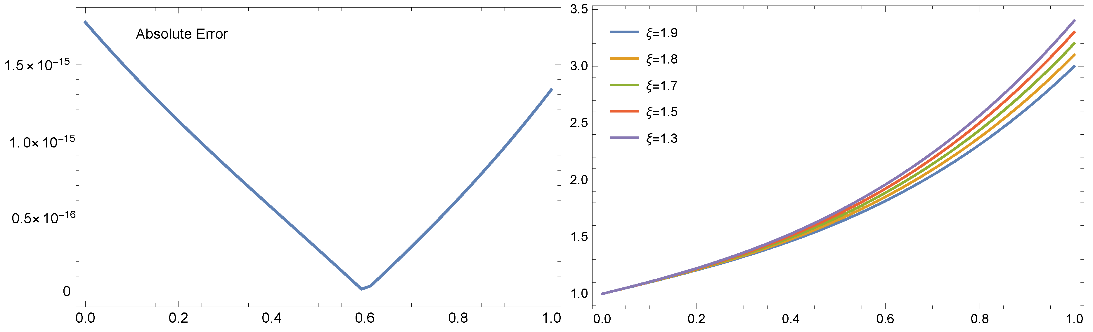
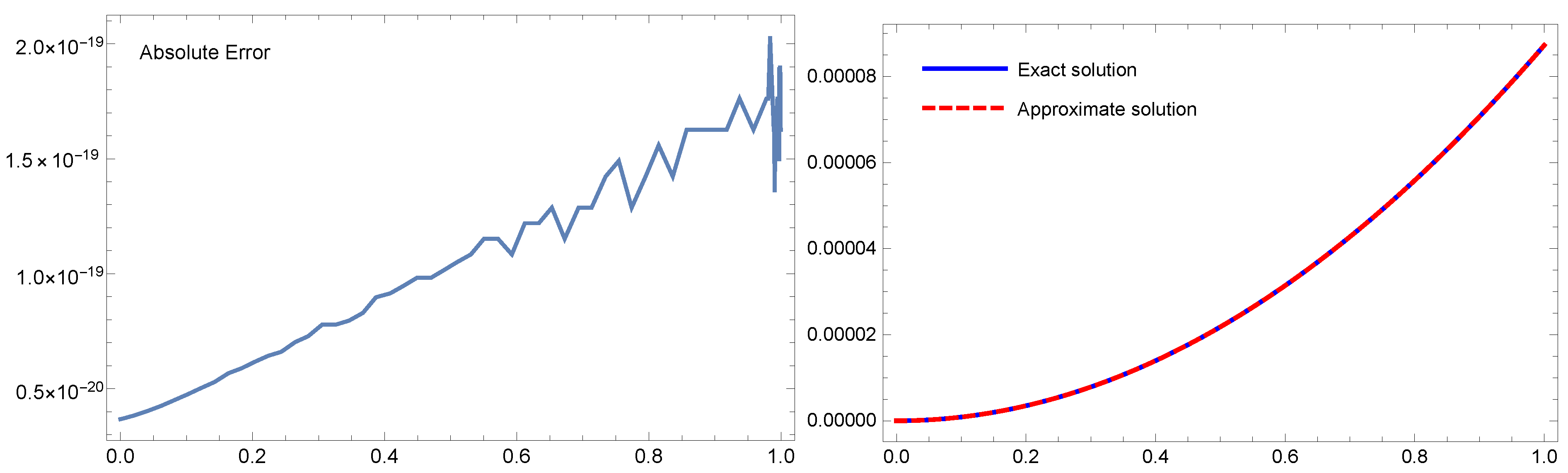
presents $L^2$-error and $L_{\infty }$-error results using our suggested method MVOMM in addition to the comparison with these results obtained via Lucas wavelet scheme (LWS) [53]. From these results, we obtain the accuracy of the proposed method. For further illustration, we introduce Figure 1, which shows the absolute error (left), and (right) the approximate solutions $\xi =1.9,1.8,1.7,1.5,1.3$ for Example 1 with $m=3$. Clearly, from Figure 1, the accuracy and efficiency of the MVOMM is useful for obtaining the numerical solutions in several cases. In addition, it can be noticed from the figure that while changing the value of the fractional order $\xi$, the value of the solution is increasing. This proves that the change in the fractional order has an impact on the simulation of the results.

Example 2 

([51]). In our next experiment, we will show that MVOM method can handle problems with discontinuities. To keep things simple, we will consider a model problem that only has one discontinuous point, but it is possible to extend the method to handle a larger number of discontinuities. We will consider a fractional-order Bagley–Torvik equation with an initial value and a discontinuous right-hand side.

$${\mathbb{D}}^{2}g\left(t\right)+{\mathbb{D}}^{1.5}g\left(t\right)+g\left(t\right)=\vartheta \left(t\right),t\in (0,2),g\left(0\right)=g^{\prime }\left(0\right)=0,$$

(31)

where

$$\vartheta \left(t\right)=\left\{\begin{array}{cc}\hfill 2+t^2+\frac{4t^{0.5}}{\sqrt{\pi }},\hfill & \hfill 0\le t<t_1,\hfill \\ \hfill 1+7t+t^3+\frac{8t^{1.5}}{\sqrt{\pi }},\hfill & \hfill t_1\le t\le t_2.\hfill \end{array}\right.$$

In this case, $t_1$ is a point where the discontinuity occurs. The exact solutions to the problem are $g\left(t\right)=t^2$ for the variable t in the interval $I_1=[0,t_1)$ and $g\left(t\right)=t(t^2+1)+1$ for t in the interval $I_2=[t_1,t_2]$. We will assume that the discontinuous point $t_1$ coincides with a mesh node.

For the purposes of this example, we will set $I_1=[0,1)$ and $I_2=[1,2]$. Using $m=3$, we obtain the following approximations:

$$\begin{array}{ll}\hfill & g_3\left(t\right)=-4.44089\times {10}^{-16}+t^2-3.45025{10}^{-16}{t}^3,t\in I_1,\hfill \\ \hfill & g_3\left(t\right)=1+t-1.77636\times {10}^{-15}{t}^2+t^3,t\in I_2.\hfill \end{array}$$

(32)

For Example 2, through both intervals $I_1$, $I_2$ and with $m=3$, we obtain all the results via our suggested technique (MVOMM), reported in Equation (32),

Table 3. Absolute error comparisons for the presented method for Example 2, $\xi =1.5,m=3$.

$\mathit{t}\in {\mathit{I}}_1$	Absolute Errors	$\mathit{t}\in {\mathit{I}}_2$	Absolute Errors
0.0	$4.44089\times {10}^{-16}$	1.0	$8.88178\times {10}^{-15}$
0.1	$4.37773\times {10}^{-16}$	1.1	$8.70304\times {10}^{-15}$
0.2	$4.20204\times {10}^{-16}$	1.2	$8.51763\times {10}^{-15}$
0.3	$3.93453\times {10}^{-16}$	1.3	$8.31890\times {10}^{-15}$
0.4	$3.59589\times {10}^{-16}$	1.4	$8.10019\times {10}^{-15}$
0.5	$3.20684\times {10}^{-16}$	1.5	$7.85483\times {10}^{-15}$
0.6	$2.78806\times {10}^{-16}$	1.6	$7.57616\times {10}^{-15}$
0.7	$2.36027\times {10}^{-16}$	1.7	$7.25753\times {10}^{-15}$
0.8	$1.94416\times {10}^{-16}$	1.8	$6.89226\times {10}^{-15}$
0.9	$1.56044\times {10}^{-16}$	1.9	$6.47371\times {10}^{-15}$
1.0	−	2.0	$5.99520\times {10}^{-15}$

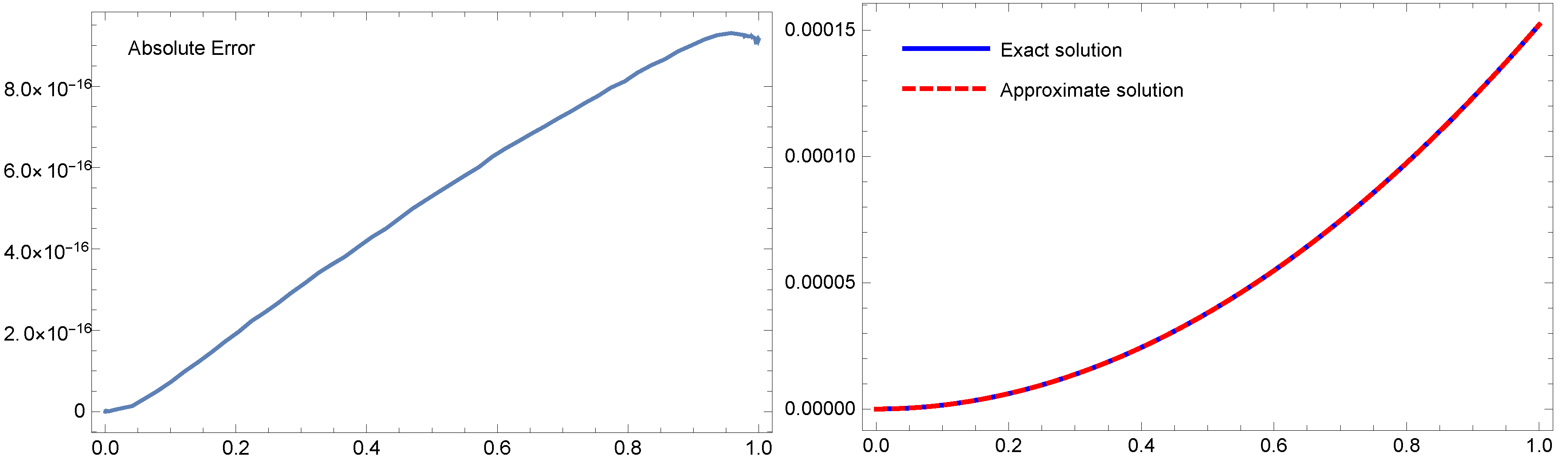
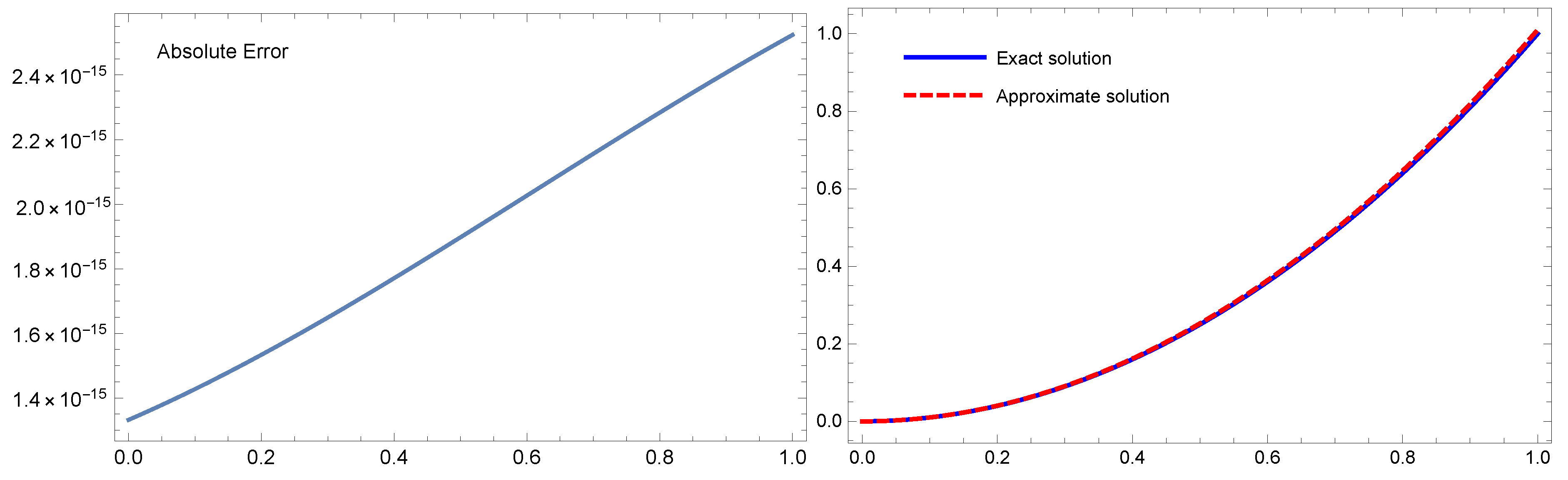
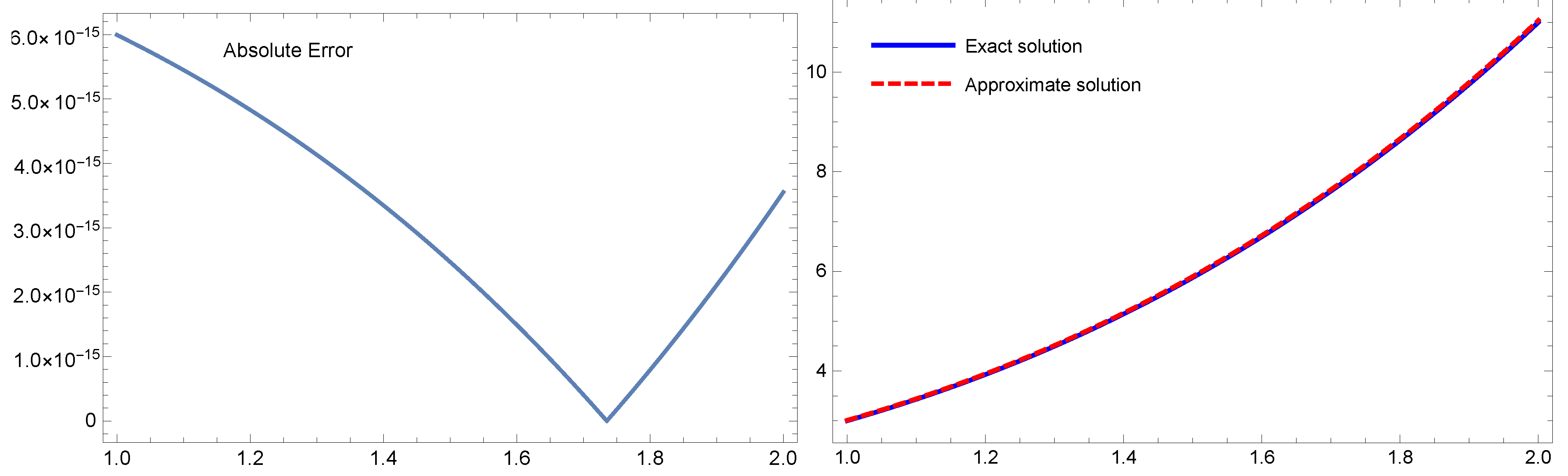
, Figure 2 and Figure 3. The results that were obtained by Equation (32) indicate the approximate solutions were approximately consistent with the analytical solutions. Table 3 represented the absolute error, which is very tiny. Figure 2 shows the exact and approximate solutions (right), and the absolute error (left) at $t\in I_1$. Figure 3 presents the exact and approximate solutions (right), and the absolute error (left) where $t\in I_2$. Moreover, when $m=3$, the CPU time required to produce these results at $t\in I_1$, $t\in I_2$ are $0.720$ s, $0.858$ s, respectively. Based on the presented results, we can say that our proposed algorithm gives high accuracy and efficiency.

Example 3 

([51]). For the last examination, we choose a case study that is representative of the types of issues encountered in the modeling of electrical and mechanical oscillations, in order to make the example more applicable and realistic to real-world situations:

$$a_1{\mathbb{D}}^{2}g\left(t\right)+a_{2}g\left(t\right)=f_{0}cos\left(\varrho t\right),f_0,\varrho >0,$$

(33)

with the original state

$$g\left(0\right)=g_0,g^{\prime }\left(0\right)=0,0<t\le \tau .$$

In our analysis of Equation (33), we only considered the cases where the forcing function is a sinusoidal wave with an amplitude of $f_0$ and a frequency of $\varrho$. Using the MVOM scheme, we examined three different vibration problems for $a_1$ and $a_2$ values of 1. We obtain the numerical solution for these cases as the following:

• Case I: $f_0=0,g_0=1,$ and $\tau =1$. The analytical solution is $g\left(t\right)=cos\left(t\right)$.
• Case II: $f_0=0.01,g_0=0,\varrho =1,$ and $\tau =1$. The precise solution $g\left(t\right)=0.005tsin\left(t\right)$.
• Case III: $f_0=1,g_0=0,$ and $\tau =1$. The true solution is $g\left(t\right)=\frac{1}{1-{\varrho }^2}\left(cos\left(\varrho t\right)-cos\left(t\right)\right)$,
  where ${\varrho }^2\ne 1$. Here, we have $\varrho =6$.

The proposed approach that was explained in the preceding Section is used to compute the absolute error for the three cases of Example 3. It is visible from analyzing the outcomes of

Table 4. Absolute error comparisons for the presented method for Example 3.

	Case I		Case II		Case III
t	LDG [51]	MVOMM $(\mathit{m}=4)$	LDG [51]	MVOMM $(\mathit{m}=4)$	LDG [51]	MVOMM $(\mathit{m}=6)$
0.0	−	$2.22\times {10}^{-16}$	−	$2.42\times {10}^{-20}$	−	$3.95\times {10}^{-20}$
0.1	$1.95\times {10}^{-8}$	$4.44\times {10}^{-16}$	$7.76\times {10}^{-10}$	$1.14\times {10}^{-15}$	$1.12\times {10}^{-9}$	$7.12\times {10}^{-17}$
0.2	$1.36\times {10}^{-8}$	$1.89\times {10}^{-15}$	$5.38\times {10}^{-10}$	$3.58\times {10}^{-15}$	$5.91\times {10}^{-10}$	$1.92\times {10}^{-16}$
0.3	$9.66\times {10}^{-9}$	$3.33\times {10}^{-15}$	$3.79\times {10}^{-10}$	$6.32\times {10}^{-15}$	$1.92\times {10}^{-8}$	$3.07\times {10}^{-16}$
0.4	$9.96\times {10}^{-9}$	$4.89\times {10}^{-15}$	$3.94\times {10}^{-10}$	$8.86\times {10}^{-15}$	$3.11\times {10}^{-8}$	$4.18\times {10}^{-16}$
0.5	$1.02\times {10}^{-8}$	$6.22\times {10}^{-15}$	$4.01\times {10}^{-10}$	$1.11\times {10}^{-14}$	$1.92\times {10}^{-8}$	$5.31\times {10}^{-16}$
0.6	$5.06\times {10}^{-9}$	$7.44\times {10}^{-15}$	$2.01\times {10}^{-10}$	$1.33\times {10}^{-14}$	$5.55\times {10}^{-9}$	$6.33\times {10}^{-16}$
0.7	$9.44\times {10}^{-9}$	$8.77\times {10}^{-15}$	$3.72\times {10}^{-10}$	$1.55\times {10}^{-14}$	$1.88\times {10}^{-8}$	$7.27\times {10}^{-16}$
0.8	$3.58\times {10}^{-9}$	$1.01\times {10}^{-14}$	$1.42\times {10}^{-10}$	$1.78\times {10}^{-14}$	$1.62\times {10}^{-8}$	$8.18\times {10}^{-16}$
0.9	$4.79\times {10}^{-9}$	$1.10\times {10}^{-14}$	$1.89\times {10}^{-10}$	$1.94\times {10}^{-14}$	$9.71\times {10}^{-9}$	$9.03\times {10}^{-16}$
1.0	$3.18\times {10}^{-15}$	$1.08\times {10}^{-14}$	$1.19\times {10}^{-16}$	$1.87\times {10}^{-14}$	$1.12\times {10}^{-19}$	$9.15\times {10}^{-16}$

that were generated by the proposed methodology and the results produced by the method provided in [51] that the results provided by the proposed scheme are more accurate than those published in [51]. Additionally, the CPU time of our method is better than of [51] because we have few terms of the expansion series $m=4,6$ only. We obtain the CPU time in these different cases (Case I, Case II, and Case III), which are $0.093,0.110$, and $0.125$ s, respectively. A great degree of precision is also provided by the proposed method for solving oscillation problems.

Figure 4, Figure 5 and Figure 6 are reported at $m=6$ for Example 3 through three different cases of oscillations. Figure 4 gives the absolute error on left, the analytic and an approximation solutions on right for Case I. Figure 5 presents the absolute error on left, the exact and numerical solutions on right for Case II. Figure 6 indicates the absolute error on left, the exact and an approximation solutions on right for Case III. At first glance of these three figures, we notice a great degree of agreement between the exact and the numerical solution.

Example 4 

([53,54]). Let us select the initial-value Bagley–Torvik equation of the fractional order

$$\begin{array}{ll}\hfill & {\mathbb{D}}^{2}g\left(t\right)+{\mathbb{D}}^{1.5}g\left(t\right)+g\left(t\right)=\vartheta \left(t\right),t\in [0,1],\hfill \\ \hfill & \vartheta \left(t\right)=t^3+\frac{8}{\sqrt{\pi }}{t}^{\frac{3}{2}}+5t,\hfill \end{array}$$

(34)

with the boundary conditions

$$g\left(0\right)=g\left(1\right)=0.$$

The corresponding exact solution for Example 4 takes the form $g\left(t\right)=t^3-t$.

We use the suggested method for solving this problem numerically. Additionally, some comparisons are made between the obtained results of MVOMM and the LWS and the reproducing kernel Hilbert space (RKHS) reported in [53,54]. By using the LWS, the obtained solution is [53]

$${\overline{g}}_3\left(t\right)=t^3-2.33591\times {10}^{-13}{t}^2-t+2.22045\times {10}^{-16}.$$

While the results with $m=3$ using our method are as follows:

$$g_3\left(t\right)=t^3-2.66454\times {10}^{-15}{t}^2-t.$$

(35)

For Example 4 at $m=3$, we acquire all findings using our recommended technique (MVOMM), which is provided in Equation (35),

Table 5. Comparison of the present study’s exact solution with the absolute inaccuracy of the RKHS [54] and LWS [53], relative to Example 4.

t	Exact	RKHS [54] $(\mathit{n}=20)$	RKHS [54] $(\mathit{n}=40)$	LWS [53] $(\mathit{H}=4)$	MVOMM $(\mathit{m}=3)$
0.2	$-0.192000$	$1.890\times {10}^{-4}$	$5.700\times {10}^{-5}$	$9.575\times {10}^{-15}$	$4.547\times {10}^{-16}$
0.4	$-0.336000$	$2.537\times {10}^{-4}$	$7.131\times {10}^{-5}$	$3.758\times {10}^{-14}$	$1.080\times {10}^{-15}$
0.6	$-0.384000$	$2.168\times {10}^{-4}$	$5.992\times {10}^{-5}$	$8.426\times {10}^{-14}$	$1.833\times {10}^{-15}$
0.8	$-0.288000$	$1.198\times {10}^{-4}$	$3.312\times {10}^{-5}$	$1.497\times {10}^{-13}$	$2.672\times {10}^{-15}$
1.0	0	0	0	0	0

,

Table 6. Comparison between the LWS introduced in [53] and the current study for Example 4 with various errors.

Error Type	LWS [53] $(\mathit{k}=0,\mathit{H}=4)$	LWS [53] $(\mathit{k}=1,\mathit{H}=4)$	MVOMM $(\mathit{m}=3)$
$L^2$-error	$8.5\times {10}^{-14}$	$2.2\times {10}^{-13}$	$3.55\times {10}^{-15}$
$L_{\infty }$-error	$1.6\times {10}^{-13}$	$5.0\times {10}^{-13}$	$1.88\times {10}^{-15}$

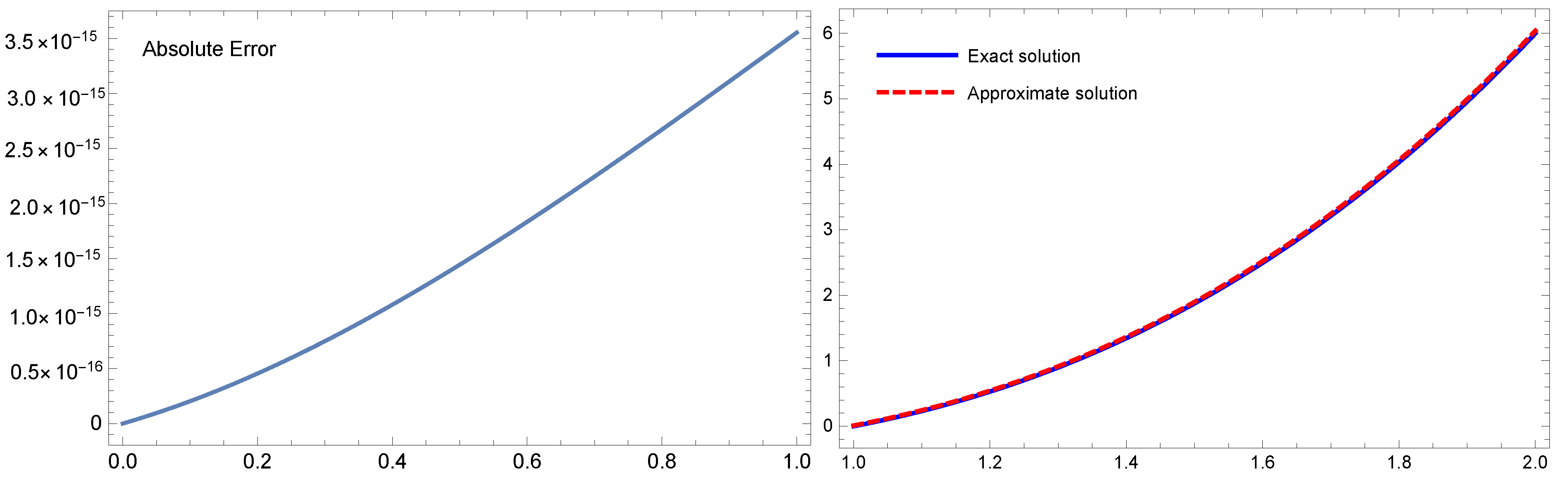
and Figure 7. Equation (35) shows that the approximations were roughly congruent with the analytical solutions. Table 5, represented a comparison of the present study’s exact solution with the absolute inaccuracy of the techniques developed in [53,54]. Table 6, displays findings for $L^2$-error and $L^{\infty }$-error utilizing our recommended approach MVOMM as well as a comparison to results obtained via [53]. Figure 7 presents the absolute error (left) and the numerical and true solutions (right). All results are obtained with CPU time $0.813$ s (including all numerical results and plotting the figures). The results derived from these Tables and Figures for Example 4 provide a strong indication of the superiority of the presented Tau-collocation algorithm. In terms of accuracy and efficiency, the proposed method was found to outperform the other methods considered.

Example 5 

([55,56,57]). Finally, we turn our attention to another form of equation, which is know as the fractional-order Bratu differential equation type:

$${\mathbb{D}}^{\xi }g\left(t\right)-2e^{g\left(t\right)}=0,t\in [0,1],\xi \in (1,2],$$

(36)

with the initial conditions

$$g\left(0\right)=g^{\prime }\left(0\right)=0.$$

The exact solution that corresponds to Example 5 at $\xi =2$ is $g\left(t\right)=-2ln(cos(t\left)\right)$.

The following results are obtained by applying our recommended approach for solving this problem numerically and comparing the outcomes with those reported in [55,56,57]. The developed methods are the compact finite difference method (CFDM), the reproducing kernel Hilbert space method (RKM), and the combined spectral Bessel quasilinearization method (Bessel-QLM), respectively. For Example 5, we obtain all the results utilizing our advised method (MVOMM), and these are presented in

Table 7. Comparison of the absolute inaccuracy between the MVOMM and the CFDM and RKM used in the previous studies [55,56,57] using $\xi =2$ for Example 5.

t	CFDM [55]	RKM [56]	Bessel-QLM $(\mathit{M}=7)$ [57]	MVOMM $(\mathit{m}=6)$
$0.1$	$7.1\times {10}^{-6}$	$1.67\times {10}^{-5}$	$4.20\times {10}^{-8}$	$2.75\times {10}^{-17}$
$0.2$	$1.23\times {10}^{-5}$	$3.10\times {10}^{-7}$	$1.22\times {10}^{-7}$	$3.016\times {10}^{-17}$
$0.3$	$1.71\times {10}^{-5}$	$1.13\times {10}^{-6}$	$1.86\times {10}^{-7}$	$1.65\times {10}^{-16}$
$0.4$	$2.26\times {10}^{-5}$	$2.12\times {10}^{-4}$	$2.61\times {10}^{-7}$	$1.87\times {10}^{-16}$
$0.5$	$2.90\times {10}^{-5}$	$2.90\times {10}^{-6}$	$3.55\times {10}^{-7}$	$8.05\times {10}^{-17}$
$0.6$	$3.69\times {10}^{-5}$	$4.10\times {10}^{-6}$	$4.10\times {10}^{-7}$	$1.32\times {10}^{-16}$
$0.7$	$4.72\times {10}^{-5}$	$6.50\times {10}^{-6}$	$5.79\times {10}^{-7}$	$2.19\times {10}^{-16}$
$0.8$	$6.14\times {10}^{-5}$	$7.50\times {10}^{-6}$	$6.83\times {10}^{-7}$	$1.67\times {10}^{-16}$
$0.9$	$8.32\times {10}^{-5}$	$3.35\times {10}^{-6}$	$3.04\times {10}^{-7}$	$2.79\times {10}^{-16}$
$1.0$	$1.29\times {10}^{-5}$	$4.37\times {10}^{-8}$	$3.23\times {10}^{-5}$	$2.52\times {10}^{-16}$

and

Table 8. Comparison of the highest absolute errors for Example 5 using $\xi =2$ and various values of m from [55] and our proposed approach.

CFDM [55]		MVOMM
$N=m$	$L_{\infty }$-Error	$m$	$L_{\infty }$-Error	CPU Time (s)
5	$1.67\times {10}^{-3}$	2	$1.42\times {10}^{-8}$	$0.185$
10	$8.32\times {10}^{-5}$	4	$5.61\times {10}^{-13}$	$0.225$
20	$4.43\times {10}^{-6}$	6	$4.11\times {10}^{-16}$	$0.282$
40	$2.38\times {10}^{-7}$	8	$8.34\times {10}^{-16}$	$0.586$
80	$1.36\times {10}^{-8}$	10	$1.47\times {10}^{-16}$	$1.592$

and Figure 8. Table 7, introducing comparisons of the absolute error between the current methodology and the other research approaches, CFDM and RKM published in [55,56] with $m=6$. The computational time (CPU time) in the case of $m=6$ is $0.282$s using our suggested method. Table 8 reported a comparison between the recommended approach MVOMM and this given in [55] with $L^2$-error and $L^{\infty }$-error at $\xi =2$ and diverse values of m. Additionally, the CPU time in different values of m is reported in the last column of Table 8. 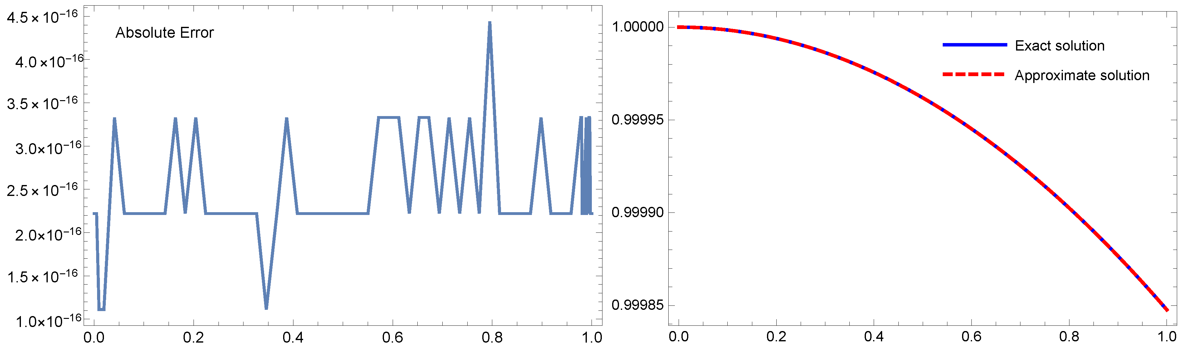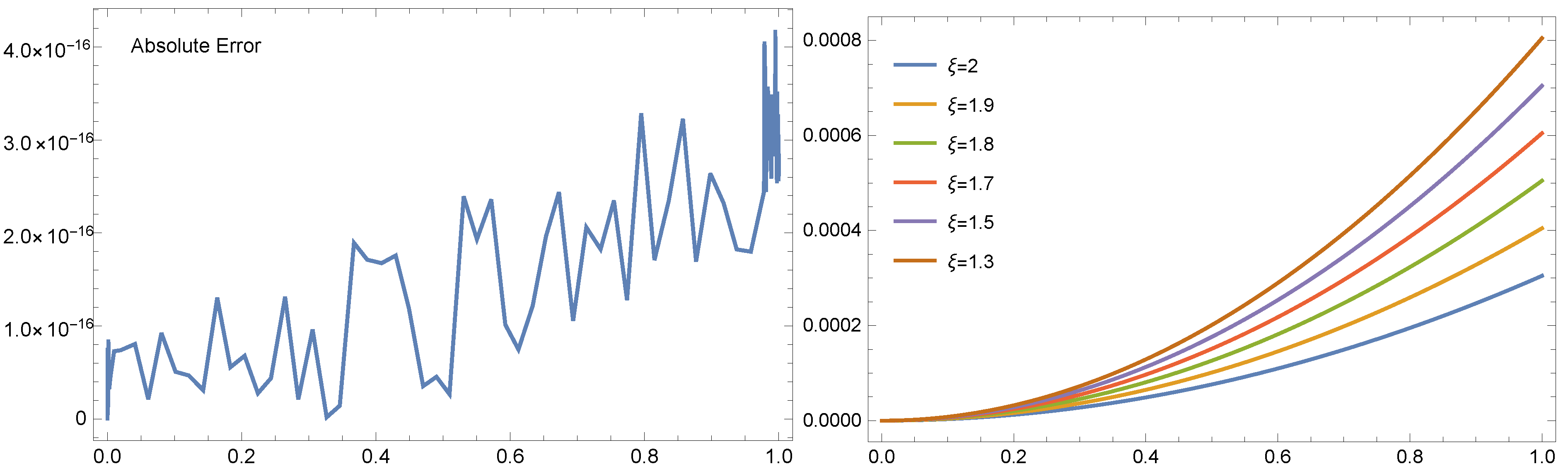Figure 8, listed the achieved absolute error for $\xi =2$ (left) and the numerical values at several values of the fractional-order term $\xi =2,1.9,1.8,1.7,1.5,1.3$ (right) with $m=6$. These Tables and Figures for numerical results of Example 5 give clear evidence of the proposed method’s superiority. The proposed method was found to perform better than the other existing numerical procedures taken into consideration in terms of efficiency and accuracy.

6. Conclusions

In this research manuscript, we propose a novel technique based on the collocation strategy to acquire the approximate and numerical solutions for a class of fractional-order differential equations with various applications in science. To achieve this purpose, we utilize a novel operational matrix of fractional order for the Morgan–Voyce polynomials defined in the Liouville–Caputo sense combined with the collocation and Tau method. This approach involves converting the fractional order model into an algebraic system of equations with unknown coefficients, which are then solved to find these coefficients efficiently. A rigorous error analysis for the presented Tau-collocation technique shows that the proposed technique converges to the required solution. Several examples are illustrated to highlight the efficiency of the technique including the well-known Bagley–Torvik and Bratu equations and other models with different fractional orders. The results are compared with other relevant available techniques from the literature which support the proposition of a more accurate solution with fewer bases. These results provide insight into the behavior of the solution of the investigated models. In addition, the robustness of the proposed algorithm is verified by providing computational time which supports the claim. The method successfully provides accurate results highlighting the importance of the solved model, especially of the Bagley–Torvik model which have applications in simulating coupled oscillator. Thus, the provided methods are considered promising techniques for simulating similar models and can be extended to some more complex problems in the future including fractional partial differential equations with real-life applications.