Article

Improved Particle Swarm Optimization Fractional-System Identification Algorithm for Electro-Optical Tracking System

1
Key Laboratory of Optical Engineering, Chinese Academy of Sciences, Chengdu 610209, China
2
Institute of Optics and Electronics, Chinese Academy of Sciences, Chengdu 610209, China
3
University of Chinese Academy of Sciences, Beijing 100049, China
*
Author to whom correspondence should be addressed.
Fractal Fract. 2023, 7(3), 264; https://doi.org/10.3390/fractalfract7030264
Submission received: 6 February 2023 / Revised: 13 March 2023 / Accepted: 13 March 2023 / Published: 16 March 2023

Abstract

:
When an electro-optical tracking system (ETS) needs higher control precision, system identification can be considered to improve the accuracy of the system, so as to improve its control effect. The fractional system model of ETS can describe the characteristics of the system better and improve the accuracy of the system model. Therefore, this paper presents a fractional system identification algorithm for ETS that is based on an improved particle swarm optimization algorithm. The existence of the fractional order system of ETS was verified by identification experiments, and the fractional order system model was obtained. Under the same conditions, PI controllers were designed based on a fractional order system and an integer order system, respectively. The results verify the superiority of fractional order system in ETS.

1. Introduction

The electro-optical tracking system (ETS) is one of the critical pieces of equipment for realizing the acquisition, tracking, and pointing functions. It is a high-precision tracking and positioning device composed of the mechanical structure, photoelectric sensor, and control technology, which plays a critical role in target recognition, navigation, and positioning, as well as in aerospace, telescope systems, beam stability control, space optical communication, and quantum communication, among other domains [1]. The composite axis tracking system is an important part of the ETS, and the fast steering mirrors (FSMs) in the composite axis structure can further suppress the residual of coarse tracking, while also providing higher bandwidth and accuracy for the system, which is one of the key components of the absolute tracking accuracy. As a result, the FSM platform control is critical in implementing ETS’s high accuracy tracking and positioning capabilities [2]. With the advancement of modern technologies, the demand for ETS equipment is increasing. In the realm of quantum communication, the laser is sent from the satellite to the ground receiving device, and the propagation distance can reach 2000 km. Therefore, the propagation process will inevitably result in the loss of laser energy. In this scenario, to ensure that the receiver can receive enough energy, the tracking error of the system must be very low, and the tracking accuracy should reach the level of microradians [3,4]. Environmental conditions and control system design are currently the most important elements influencing tracking accuracy. The prior control model was relatively basic, with low accuracy, but it was unable to satisfy the requirements of the current. At the moment, the ETS model-identification approach is primarily based on frequency domain response data, with the curve fitting algorithm used to identify [5,6]. Controlling an inaccurate model is relatively difficult. To fulfill the ever-increasing model accuracy requirements, it is a necessary and crucial development direction to improve the identification and design of control systems while ignoring the impact of environmental interference and noise [7,8].
At present, ETS model identification is typically an integer order model. When the model’s order is fixed, the model’s correctness is mostly determined by the accuracy of the coefficient of the transfer function derived by the identification algorithm. However, the recent invention of fractional calculus gives a new method for system identification. The fractional-order system is described by the fractional differential equation. The concept of fractional calculus theory was first proposed in 1695 [9], but due to a lack of clear physical meaning and the lack of matching solving tools, the application research on this theory has been slow to develop. With the development of computer technology, the use of fractional calculus has gradually permeated numerous engineering applications. The authors of [10] mentioned that many systems in nature have the characteristics of a fractional system, so for a system with fractional characteristics, the fractional mathematical model is preferable to the integer mathematical model for describing system characteristics. Particularly in the frequently used sector of motors, it appears that a fractional-order system can better represent the features of RLC electronic devices [11]. Thus, many scholars have conducted studies on the identification of fractional-order systems of various types of motors and verified that the fractional order system model can better characterize a motor system’s features [12]. The FSM platform in ETS is often powered by a voice coil motor, and its motion performance is highly tied to the motor’s properties. The traditional integer-order modeling method is used to model the fast mirror system, so the driving link is still described by the integer-order equation, which cannot adequately explain the mechanical and electrical features of the system. As a result, it is necessary to verify the existence of the fractional characteristics in the ETS and to establish the fractional system model of the ETS based on the fractional calculus theory so as to better characterize the system characteristics, improve the system identification accuracy, and ultimately improve the system control performance.
For fractional systems, numerous identification methods have been devised. The time domain or the frequency domain can be used for parametric identification of fractional-order systems [13,14,15,16,17,18,19]. In comparison to an integer-order system, a fractional-order system needs to estimate the numerator and denominator polynomial coefficients, as well as identify the order coefficients, increasing the difficulty of the identification task. It is an efficient method for converting an identification problem into an optimization problem. Some scholars have used the particle swarm optimization algorithm to identify fractional-order systems [20,21]. Unfortunately, in system identification, a large number of differential operations are required, which greatly limits the running speed of the optimization algorithm. Because the ETS is easily affected by ambient elements such as location and temperature in practical applications, and often loaded in the motion platform for use [22], it is frequently required to precisely identify the model in time.
In this paper, an enhanced particle swarm optimization identification algorithm based on a fractional model of ETS is proposed. This method makes use of the block pulse function property to improve the efficiency of identification [23]. By enhancing the performance index function of the particle swarm optimization algorithm, the algorithm’s computing performance is considerably improved. Furthermore, when the identification errors of the fractional order model are compared to those of the integer order model, the identification accuracy of the fractional order model is clearly better than that of the integer-order system, and the identification mean square error is reduced by 56.9%, proving the existence of the ETS’s fractional order model. The PI controller is then developed using the fractional-order system and the integer-order system, respectively, and the control impact is evaluated on the actual platform. Lastly, it is demonstrated that a PI controller developed on a fractional-order system can provide a greater control effect under the same open-loop correction limitations. This demonstrates that using a fractional system model on the ETS has more advantages, and it also serves as a foundation for the later design of a fractional system-based controller. This paper’s primary contributions are as follows:
(1) To address the issue of tracking precision being limited by the low accuracy of the system model in the ETS, a fractional model of ETS is presented. Moreover, the fractional-order system model is proved to be more accurate than the integer-order system model.
(2) To solve the problem that the present fractional model identification methodology has a sluggish identification speed, an improved particle swarm optimization algorithm is proposed, and the advantages of the method in running speed are proved by simulation.
(3) It is demonstrated that a fractional system model can have superior control performance to an integer system model with the same crossing frequency and phase margin by building a PI controller for fractional system model.
This paper is organized as follows: Section 2 discusses the mathematical and theoretical tools used in this paper. Section 3 briefly introduces the ETS model. The improved identification algorithm is shown in Section 4. Section 5 validates the algorithm’s operating speed and identification accuracy using simulation and experimentation. Section 6 shows the control impact of the actual platform. The seventh section is an article summary.

2. Mathematical Preliminaries

2.1. Definitions of Fractional Derivatives and Integrals

Fractional calculus is a generalization of integral calculus and is defined as follows [24]:
a D t α = d α d t α , α > 0 1 , α = 0 a t ( d τ ) α , α < 0
where a and t are the limits and α is the order of the operation. Currently, there are several different definitions of fractional calculus. Examples include Caputo definitions, G-L definitions, R-L definitions, and so on [25]. Within the scope of this paper, these definitions are equivalent, so we chose the definition of R-L to carry out fractional calculus, which is defined as follows:
a D t α f ( t ) = 1 Γ ( n α ) d d t n a t f ( τ ) ( t τ ) α + 1 n d τ
where Γ ( · ) is Euler’s Gamma function and n 1 < α < n , n N . The fractional integration of R–L is given by
I a α f ( t ) = 1 Γ ( α ) a t f ( τ ) ( t τ ) 1 α d τ
where t > a and α is the real positive integration order.

2.2. The Laplace Transform of Fractional Derivative

The Laplace transform is an important tool to describe fractional calculus. The Laplace transform of the R-L fractional derivative is defined as [26]:
L 0 D t α f ( t ) = s α F ( s ) k = 0 n 1 s k 0 D t α k 1 f ( t ) t = 0
Under zero initial condition, the Laplace transform of the fractional derivative is simplified as
L 0 D t α f ( t ) = s α F ( s )
The Laplace transform of the fractional integral under zero initial condition is given as
L I 0 α f ( t ) = 1 S α F ( s )

2.3. Mathematical Description of Fractional Systems

For a continuous-time linear time-invariant system with input signal u ( t ) and output signal y ( t ) , the general form of the linear SISO system described by fractional differential equation can be obtained by using fractional differential operators [27]
a n D α n y ( t ) + a n 1 D α n 1 y ( t ) + + a 0 D α 0 y ( t ) = b m D β m u ( t ) + b m 1 D β m 1 u ( t ) + + b 0 D β 0 u ( t )
Among them, each order satisfies α n > α n 1 > > α 0 , β m > β m 1 > > β 0 .
When the initial conditions of input u ( t ) and output y ( t ) are all zero in system (7), the transfer function expression of the system can be obtained by using the Laplace transform:
G ( s ) = Y ( s ) U ( s ) = b m s β m + b m 1 s β m 1 + + b 0 s β 0 a n s α n + a n 1 s α n 1 + + a 0 s α 0 .

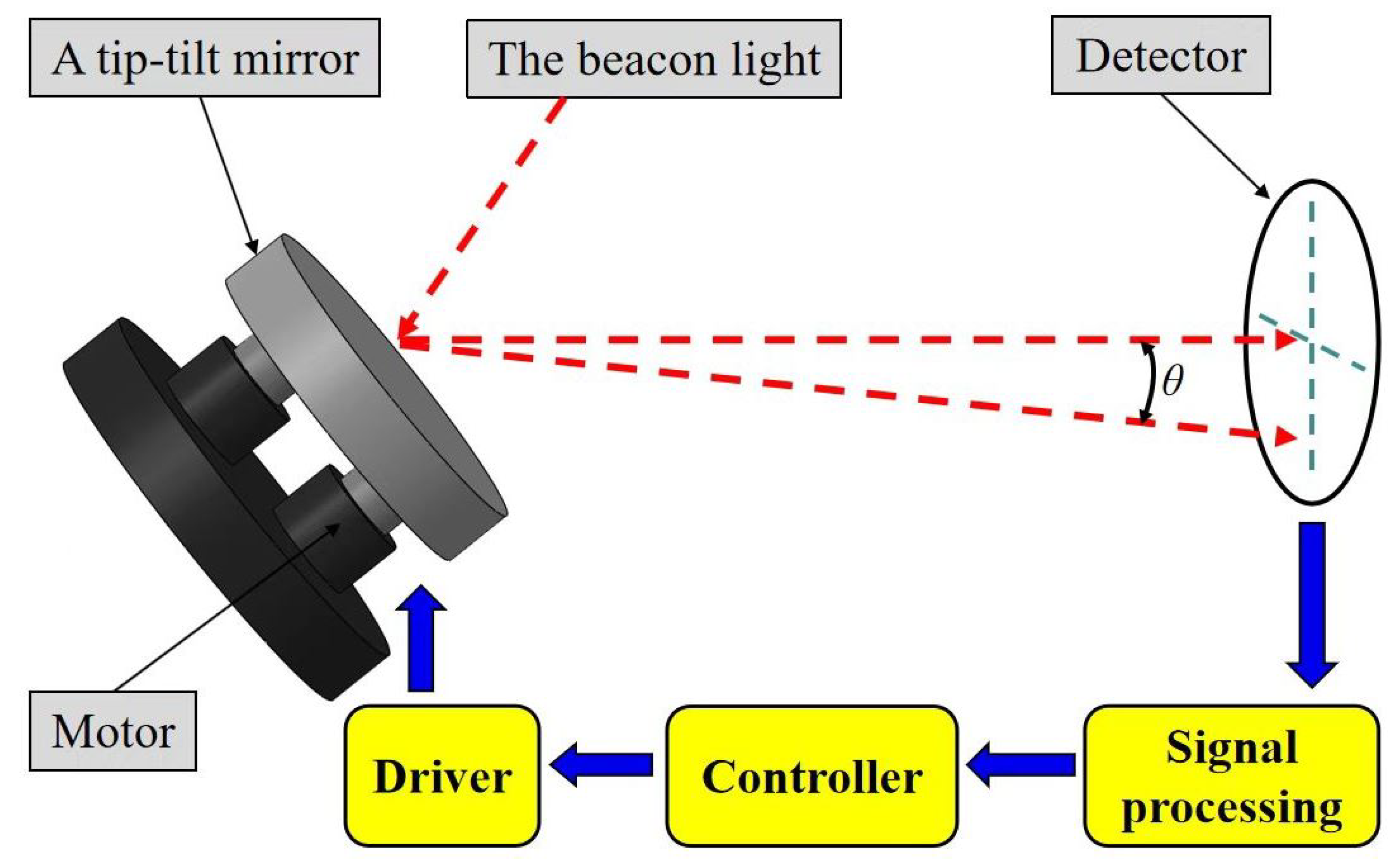
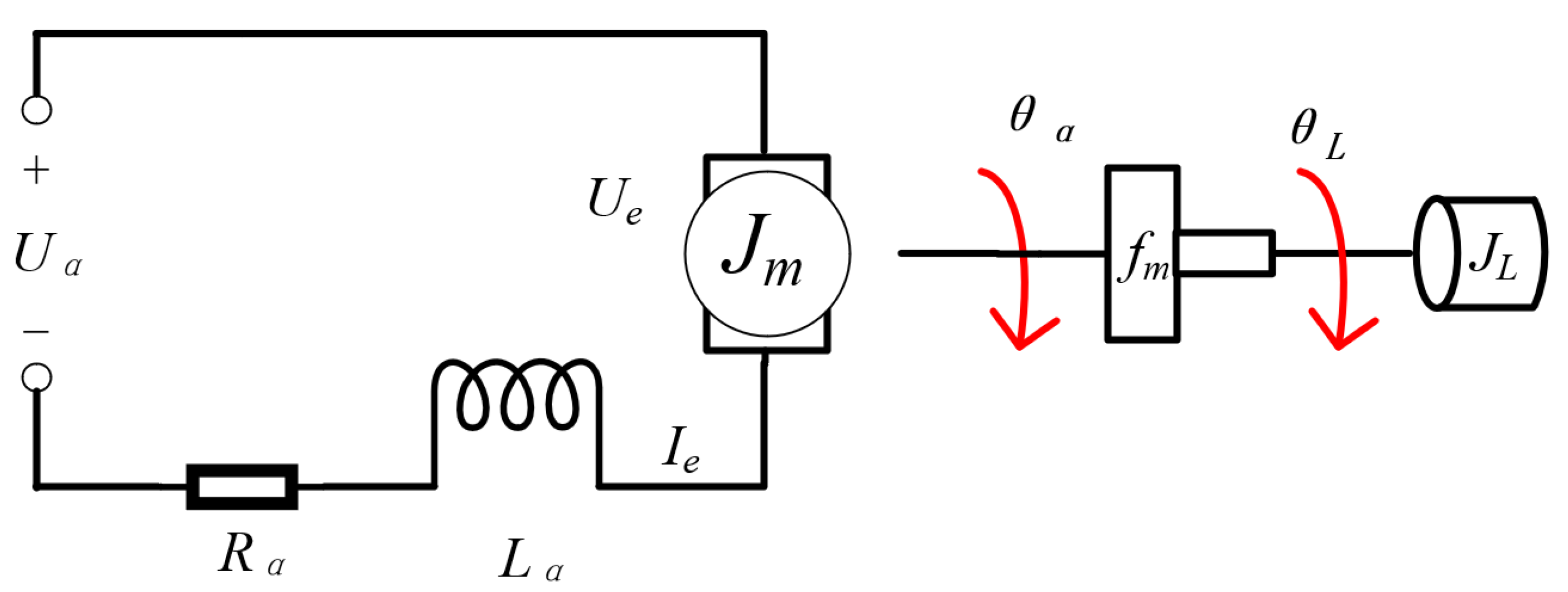
3. ETS Model Analysis

The ETS based on the FSM is shown in Figure 1, composed of a two-dimensional mirror, image detector, controller, digital signal processor, power drive amplifier, drive motor, etc. The deflection direction of the mirror is adjusted through four motors to control the beam deflection angle and then reflect the beacon light to the target detector. In Figure 2, using the potential and torque balance equation, we can obtain [28]
U a = R a I a + L a I ˙ a + K b θ ˙ C m I a = J L θ ¨ + f m θ ˙ + K m θ ,
where U a , I a , R a , L a , K b , C m , f m , and K m are voltage, current, resistance, inductance, back EMF coefficient, torque coefficient, viscous friction, and spring stiffness of motor, respectively. Considering that the armature inductance of the motor is relatively small, the model is further simplified. If L a 0 , we can obtain
U a = R a I a + K b θ ˙ C m I a = J L θ ¨ + f m θ ˙ + K m θ
The corresponding integer-order transfer function can be given as follows:
G i o ( s ) = k s 2 + a s + b
where a = R a f m + K b C m J L R a , b = K m J L and k = C m J L R a . In [11], the results show that different arrangements of RLC (Resistance inductance and capacitance) devices may lead to non-integer behavior. Therefore, considering the fact that the electrical characteristics of the capacitor and inductor are fractional, the order of the system should be replaced by a fractional order:
G f o ( s ) = k s α + a s β + b
where α and β are any real numbers greater than 0. We thereby obtain the fractional model of the ETS. When we obtain the integer order model (11) and fractional order model (12), we can find that model (11) is a special case of model (12). The model (11) has a fixed order and simple form and few parameters to be identified. The order of model (12) is not fixed, the form is complex, and more parameters need to be identified, but this also improves the granularity and freedom of identification. The fractional-order model (12) can describe the characteristics of ETS more accurately than the integer-order model (11), since this fractional-order feature in model (12) is closer to the nature of the components in ETS. In order to solve the more difficult fractional system identification problem, we propose a new optimization algorithm method in the next section.

4. Improved Particle Swarm Optimization Algorithm

4.1. Particle Swarm Optimization Algorithm

Particle swarm optimization, which was developed in 1995 [29], can be used to find nonlinear fractional-order systems. In particle swarm optimization, each particle remembers its own previous best value, as well as the best value in its neighborhood, and uses the most successful information to improve itself, with high storage capacity and efficiency. Particle swarm optimization has three characteristics, namely fitness, position, and speed. The fitness value is used to assess particle quality.
Each particle in M-dimensional space represents the point at the intersection of all search dimensions. The particles in the population are transported to the optimal point by adding velocity to their positions. The velocity of particles is updated by inertia, cognition, and society. The inertial component simulates the particle’s previous inertial behavior; the birds’ memory of their previous best position is modeled by a cognitive component model; the birds’ memory of the best position in the particle is modeled by the social component; and the particle moves through the M-dimensional search space until it finds the best solution.
The velocity update equation is
V i m = w V i m + c 1 r 1 P i m X i m + c 2 r 2 P g m X i m
The position update equation is
X i m = X i m + V i m
where V i m , X i m is the velocity and position of the number i particle in m-dimensional space; w is inertial weight; c 1 and c 2 are weighted coefficients; P i m is the optimal position for the individual particles; P g m is the optimal particle in the population; m is the dimension of optimization problem; r 1 and r 2 are two independently generated uniformly distributed random numbers within the range of [ 0 , 1 ] .
After setting the operating environment of the particle swarm optimization algorithm, we can use the following performance index function to identify the fractional-order system:
J = 1 L t = 1 L [ y ( t ) y ^ ( t ) ] 2
y ( t ) is the time domain output data of the measured system, y ^ ( t ) is the time domain system estimate output data, and L is the number of data point used for the identification. The time domain performance index function J reflects the quality of the identification results. According to Equation (12), when identifying the ETS, the parameters to be identified in J include the fractional order and the coefficient of the system model. In order to improve the running speed of the algorithm, we will improve the performance index function in the next subsection of the article.
Remark 1.
J is a performance index function in the form of mean square error, which can reflect the difference between the estimated value and the real value. In the identification process, a smaller J value represents a better identification effect [30].

4.2. Block Pulse Functions

The block pulse functions belong to a family of piecewise orthogonal functions. They are defined over the time interval [ 0 , T ] as follows:
ψ i ( t ) = 1 , i 1 M T t < i M T 0 elsewhere
where i = 1 , , M , and M is the number of elementary functions. Any function that is absolutely integrable on the interval [ 0 , T ] can be written as follows:
f ( t ) f T ψ ( M ) ( t ) = i = 1 M f i ψ i ( t )
where f T = f 1 , f 2 , , f M is the coefficient vector defined as
f i = M T 0 T f ( t ) ψ i ( t ) d t = M T ( i 1 ) T / M i T / M f ( t ) ψ i ( t ) d t
ψ ( M ) T ( t ) = ψ 1 ( t ) , ψ 2 ( t ) , , ψ M ( t ) is the block pulse basis functions vector (T denotes the transpose). Therefore, we can rewrite Equation (3) in the form of a block pulse function:
I 0 α ψ ( M ) ( t ) = 1 Γ ( α ) 0 t ( t τ ) α 1 ψ ( M ) ( τ ) d τ = 1 Γ ( α ) t α 1 ψ ( M ) ( t ) ,
where ∗ denotes convolution. After some manipulations, Equation (19) can be written in a matrix form:
I 0 α ψ ( M ) ( t ) F α ψ ( M ) ( t ) ,
where F α is called the generalized operational matrix of fractional integral [23], which is given by
F α = T M α 1 Γ ( α + 2 ) f 1 f 2 f 3 f M 0 f 1 f 2 f M 1 f 1 f M 2 0 0 f 1 M × M ,
where f 1 = 1 ,   f p = p α + 1 2 ( p 1 ) α + 1 + ( p 2 ) α + 1 . Using Equation (21), the fractional integral of any absolutely integrable function f ( t ) can be written as
I 0 α f ( t ) f T F α ψ ( M ) ( t )
In this way, the original integral operation is converted to a matrix algebra operation, so the amount of computation is significantly reduced. In the next section, we will construct the performance index function in the optimization algorithm by such an operation.

4.3. The Performance Index Function Based on Block Pulse Functions

The transfer function of a fractional-order system such as Equation (12) can be generalized as follows:
G ( s ) = Y ( s ) U ( s ) = b m s β m + b m 1 s β m 1 + + b 0 s β 0 a n s α n + a n 1 s α n 1 + + a 0 S α 0
where α i and β j are arbitrary positive real numbers, U ( s ) and Y ( s ) are the input and output of the system, respectively. The goal of fractional-order system identification is to estimate the system parameters a i , b j , and the fractional differential orders α i and β j according to the measured input and output data. First of all, dividing s α n both in numerator and denominator, one can obtain
G ( s ) = Y ( s ) U ( s ) = b m s β m α n + b m 1 s β m 1 α n + + b 0 s β 0 α n a n + a n 1 s α n 1 α n + + a 0 s α 0 α n
Applying Equation (22) to the system input and output, one can obtain
I 0 α y ( t ) Y T F α ψ M ( t )
I 0 α u ( t ) U T F α ψ M ( t )
Therefore, Equation (24) can be expressed as
Y T D ψ M ( t ) = U T N ψ M ( t ) ,
where D = a n I + a n 1 F α n α n 1 + + a 0 F α n α 0 ,
N = b m F α n β m + b m 1 F α n β m 1 + + b 0 F α n β 0 . According to Equation (27), the vector Y can be expressed as
Y T = U T N D 1
On the other hand,
y ( t ) = Y T ψ M ( t )
Substituting Equation (28) into Equation (29), one can obtain
y ( t ) = U T N D 1 ψ M ( t )
According to Equation (30), we change the calculation method of output signal y(t) from differential calculation to algebraic operation, which greatly improves the efficiency of calculation. The matrix N D 1 contains the coefficients and fractional orders of the system, which makes it easy to construct the identification algorithm.
Let a ^ i , b ^ j , α ^ i and β ^ j be the estimation of a i , b j , α i and β j , respectively. According to Equation (24), the operational matrix representation of the estimated system output can be written as:
y ^ ( t ) = U T N ^ D ^ 1 ψ M ( t )
where N ^ and D ^ are the estimations of matrices N and D. By substituting Equation (31) into Equation (15), we obtain the new form of the performance index function. The performance index function rewritten based on the block pulse function will greatly improve the running speed of the particle swarm optimization algorithm, which will be verified by simulation in the next section.

5. ETS System Identification Based on BPF-PSO

In this section, the BPF-PSO method will be utilized to determine ETS based on FSM. Because fractional calculus is an extension of integer calculus, system identification will be performed on the experimental platform’s input and output data by setting the range of parameters to generate the fractional and integer models of the system, respectively. Thus, the two models’ accuracies can be compared.

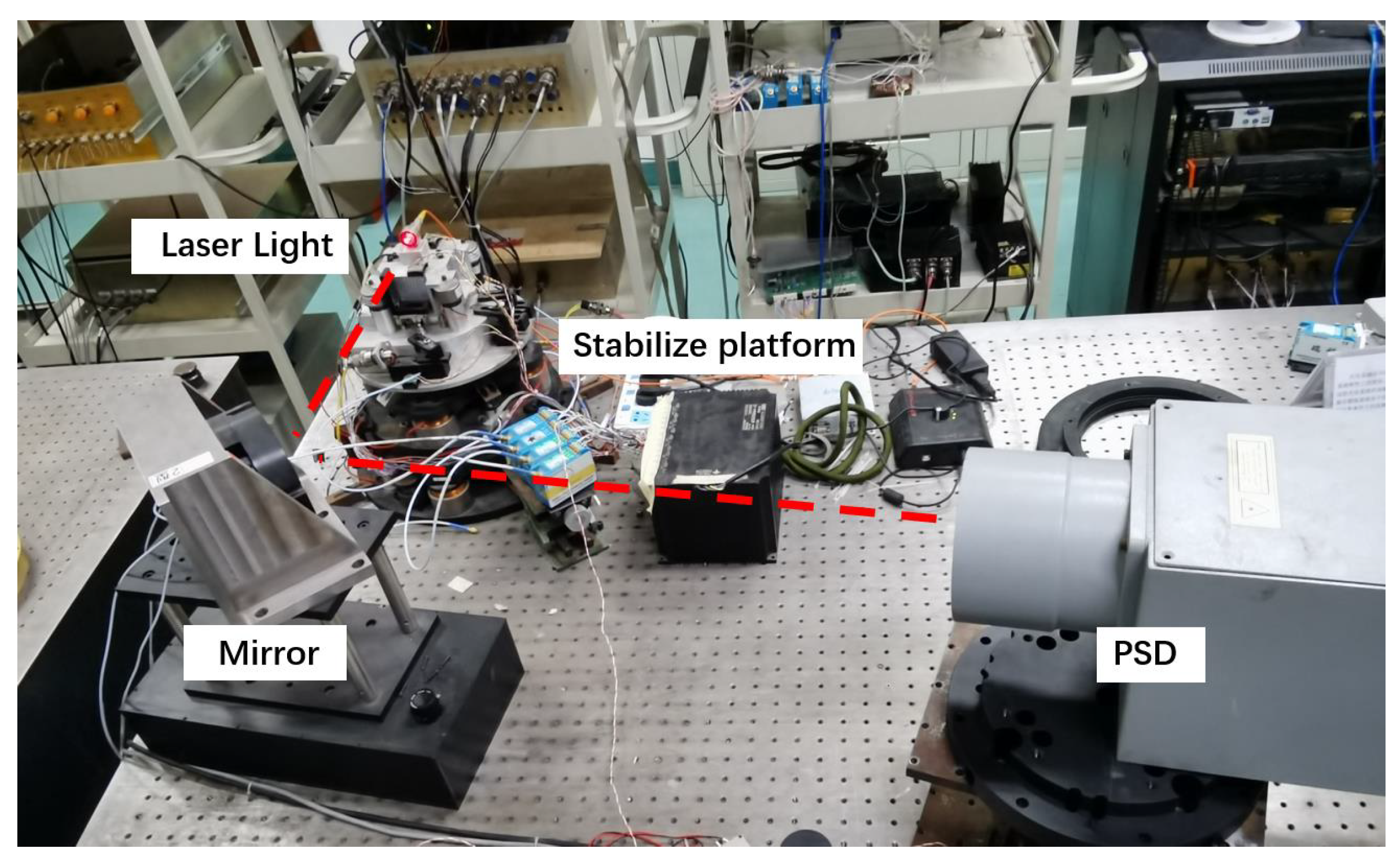
5.1. Experimental Apparatus

The FSM-based electro-optical tracking device is typically a two-axis system. Because of the symmetry of the two axes, only one of them was employed for analysis in the experiment. Figure 3 shows a laser light installed on a stable platform to imitate a moving target. A voice coil motor propels the platform. The laser light is reflected to the position-sensitive detector (PSD) by the mirror. PSD can directly output positional digital signals. In this system, the control board used was PC104LX3073 (Shenlanyu Technology Co., LTD., Shenzhen, China), on which the real-time operating system VxWorks was installed. In the experiment, the sampling rates of all the sample sensors were 5000 Hz.

5.2. Running Speed Verification

As can be seen from Equation (14), the number of elementary functions (M) is the main factor affecting the calculation speed. Moreover, when M is close to the number of sample points, the fractional-order integral calculation function rewritten by the block pulse function approximates the original function. We set different M values for the following fractional-order system and verified the identification results.
G ( s ) = Y ( s ) U ( s ) = 0.8 s 1.2 + 2 1.1 s 1.8 + 0.8 s 1.3 + 1.9 s 0.5 + 0.4
During identification, the actual number of output data in the time domain is 48,000. The number of particles in the population is 50, I m a x = 10,000 , w m a x = 0.9 , w m i n = 0.1 , c 1 = c 2 = 2 . In the experiments involved in this paper, the algorithms were run on a computer with 16G RAM. Table 1 shows the identification accuracy and time at different M.
It can be seen that when M increases, the accuracy of identification is constantly improved, but more time is spent. It can be predicted that when M approaches 48,000, in other words, when the ordinary performance index function is used instead of the performance index function based on the block pulse function, the identification time will be greatly increased. Therefore, in the actual engineering environment, the selection of appropriate M can not only meet the accuracy requirements of identification but also greatly reduce the time cost of identification.

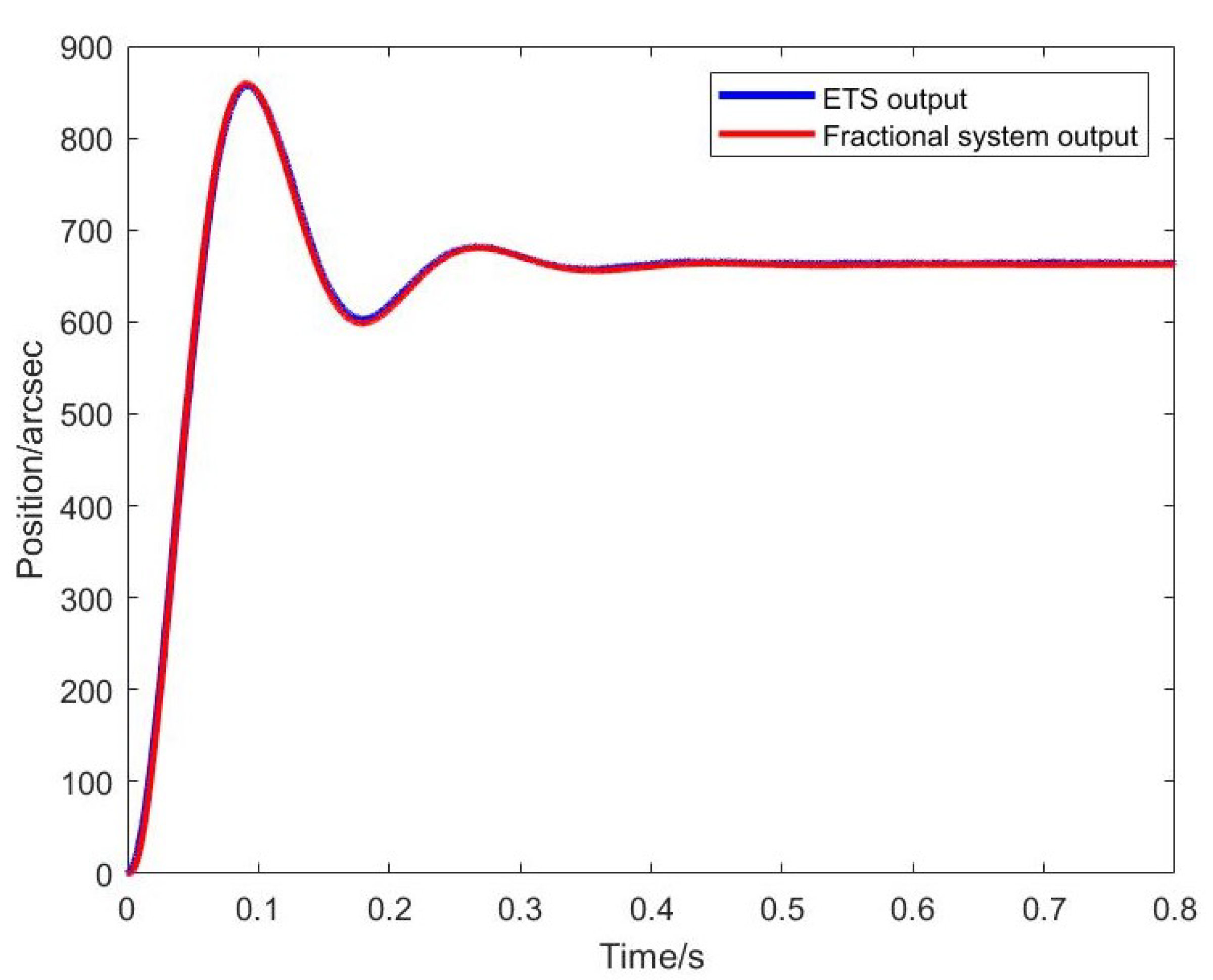
5.3. ETS Identification

The final value of step signal was set as 500 arcsec for the experiment, and 4000 data points, namely 0.8 s of data, were collected after the experiment. The results are shown in Figure 4.
The system model we need to identify is as follows:
G ( s ) = b a 2 s α 2 + a 1 s α 1 + a 0
There are six unknown parameters in this model, which are α 2 , α 1 , a 0 , a 1 , a 2 , and b. Therefore, the dimension of each particle is 6. The basis function M of the block pulse function is set to 500, the number of particles in the population is 50, I m a x = 10,000, w m a x = 0.9 , w m i n = 0.1 , and c 1 = c 2 = 2 . The minimum value of the performance index function J m i n = 7.1785 was obtained using Matlab software simulation, and the parameters of ETS fractional system model are shown in Table 2.
Therefore, we obtain the following fractional system model:
G f ( s ) = 0.06489 0.0009988 s 1.99 + 0.005014 s 0.97 + 0.04895
The fitting result is shown in Figure 5.
Next, we fixed the order of the system to α 2 = 2 and α 1 = 1 to ensure that other parameters remain unchanged and were identified again to obtain the integer order system model of the system. In this case, J m i n = 16.6514 , and the parameters of the integer order system are in Table 3.
The integer-order system model is as follows:
G i ( s ) = 0.06575 0.0009849 s 2 + 0.005127 s + 0.04961
The fitting result is shown in Figure 6.
Figure 7 shows the error analysis between the output of the two models and the output of the real system. It can be clearly seen from the following error analysis figure that the fitting effect of the fractional order system is better than that of the integer order system. From the performance index function’s value, the fitting error of the fractional order system is 56.9% lower than that of the integer-order system. It is proved that the fractional order system (34) can be closer to the real characteristics of the system than the integer order system (35).

6. Experimental Verification of the Control Performance

6.1. Tracking Performance of Fractional Order ETS

In this section, we verify the controlled effect of the object through the experimental platform. When considering system robustness and designing a robust controller, a common method is to analyze robustness based on the frequency-domain response index. Because the gain margin and phase margin reveal the relative stability of the system, they can be used to analyze the robustness of the system [31]. On this basis, we designed the controller based on the fractional-order system and integer-order system to ensure the robustness of the system. Both PI controllers are designed under the same requirements with respect to open-loop correction characteristics. The simplified control closed-loop model is shown in Figure 8.
Based on the controlled object such as Equation (12), the amplitude and phase of the controlled object are:
| G ( j ω ) | = k A ( ω ) 2 + B ( ω ) 2
Arg [ G ( j ω ) ] = arctan B ( ω ) A ( ω )
where:
A ( ω ) = ω α cos π 2 α + a ω β cos π 2 β + b
B ( ω ) = ω α sin π 2 α + a ω β sin π 2 β
The form of PI controller is as follows:
C ( s ) = K p 1 + K i s
where, K p and K i are proportional gain and integral gain respectively. The amplitude and phase of PI controller are as follows:
| C ( j ω ) | = K p 1 + K i 2 ω 2
Arg [ C ( j ω ) ] = arctan K i ω
Therefore, given the open loop gain crossing frequency ω c and phase margin φ m of the system, the equations can be listed as follows:
C j ω c G j ω c = 1
Arg C j ω c G j ω c = π + φ m
According to Equations (43) and (44), it can be solved as follows:
K i = ω c tan π φ m tan 1 B ω c A ω c
K p = ω c 2 ω c 2 + K i 2 · A ω c 2 + B ω c 2 c
In this way, we get all the parameters of the PI controller. And then, we set the system gain crossing frequency ω c = 10   rad / s ( Hz is usually used as the frequency unit in engineering applications, rad / s is used here for the convenience of controller design) and the phase margin φ m = 45 . Based on fractional order system Equation (34), we calculated PI controller parameters as follows:
C f = 1.0264 1 + 1.0704 s
The open-loop frequency domain response is shown in Figure 9.
Based on integer order system Equation (35), we calculated PI controller parameters as follows:
C i = 1.0771 1 + 0.2386 s
The open-loop frequency domain response is shown in Figure 10.
With the final step response value set to 500 arcsec and the signal input frequency set to 5000 Hz, the step response of the two systems is shown in Figure 11 and the control signal is shown in Figure 12. It can be seen that the fractional-order system responds faster than the integer-order system. Under the condition of no overshoot, the setting time of the fractional order-system is 0.495s, and that of the integer-order system is 2.379s. This is because Equations (38) and (39) are greatly simplified when the system takes integers of that order. Therefore, the fractional-order system provides a higher degree of freedom for the design of control parameters. Moreover fractional-order systems decay towards an equilibrium point such as t α , and hence the amplitude of oscillation is lesser and smoother as compared to integer-order systems. This makes the fractional order system better controlled than the integer-order system.

6.2. Experimental Platform Control Effect

On the experimental platform shown in Figure 3, we set the final step response value to 500 arcsec and the signal input frequency to 5000 Hz. The controllers designed based on the two systems are verified on the platform. The step response effect is shown in Figure 13.
It can be seen that the actual experimental results basically accord with the simulation results. The setting time of the fractional-order system is 0.4359s, and that of integer-order system is 0.8718s. The fractional-order system shows advantages in control effect.

7. Conclusions

In this research, identification method for fractional systems for ETS is proposed. The fractional-system-identification approach employs a hybrid of block pulse function and particle swarm optimization. Using identification experiments, the fractional-order system model of ETS was obtained, and it was demonstrated that the properties of the fractional-order system is closer to the genuine properties of the system than the integer order system on the same model scale. The control effect of a fractional-order system is better than that of an integer order system under identical conditions, as demonstrated by the design of a simple PI controller.

Author Contributions

Conceptualization, T.G.; methodology, Y.M.; software, T.G.; validation, T.G. and J.D.; formal analysis, X.Z.; investigation, T.G.; resources, X.Z.; data curation, J.D.; writing—original draft preparation, T.G.; writing—review and editing, J.D. and X.Z.; visualization, T.G.; supervision, Y.M.; project administration, Y.M.; All authors have read and agreed to the published version of the manuscript.

Funding

This research study was funded by the National Natural Science Foundation of China, grant numbers 61905253.

Institutional Review Board Statement

Not applicable.

Informed Consent Statement

Not applicable.

Data Availability Statement

No new data were created or analyzed in this study. Data sharing is not applicable to this article.

Conflicts of Interest

The authors declare no conflict of interest.

Abbreviations

The following abbreviations are used in this manuscript:
ETSElectro-optical tracking system
FSMFast steering mirror
PSDPosition sensitive detector

References

  1. Ulich, B.L. Overview Of Acquisition, Tracking, And Pointing System Technologies. Int. Soc. Opt. Photonics 1988, 887, 40–63. [Google Scholar]
  2. Ma, J.; Tang, T. Review of compound axis servomechanism tracking control technology. Infrared Laser Eng. 2013, 42, 218–227. [Google Scholar]
  3. Liao, S.K.; Cai, W.Q.; Liu, W.Y.; Liang, Z.; Yang, L.; Ren, J.G.; Yin, J.; Shen, Q.; Yuan, C.; Li, Z.P. Satellite-to-ground quantum key distribution. Nature 2017, 549, 43–47. [Google Scholar] [CrossRef] [PubMed] [Green Version]
  4. Yin, J.; Cao, Y.; Pan, J.W.; Li, Y.H.; Liao, S.K.; Zhang, L.; Ren, J.; Cai, W.; Liu, W.; Li, B.; et al. Satellite-based entanglement distribution over 1200 kilometers. Science 2017, 356, 1140–1144. [Google Scholar] [CrossRef] [PubMed] [Green Version]
  5. Hu, H.; Ma, J.; Wang, Q.; Wu, Q. Identification of transfer function in fast control mirror system. Opto-Electron. Eng. 2005, 32, 4. [Google Scholar]
  6. Wang, S.; Chen, T.; Li, H.; Wang, J. Frequency characteristic test and model identification of photoelectric tracking servo system. Opt. Precis. Eng. 2009, 17, 79–84. [Google Scholar]
  7. Li, J.; Chen, K.; Peng, Q.; Wang, Z.; Jiang, Y.; Fu, C.; Ren, G. Improvement of pointing accuracy for Risley prisms by parameter identification. Appl. Opt. 2017, 56, 7358–7366. [Google Scholar] [CrossRef]
  8. Huang, L.; Ma, X.; Bian, Q.; Li, T.; Zhou, C.; Gong, M. High-precision system identification method for a deformable mirror in wavefront control. Appl. Opt. 2015, 54, 4313–4317. [Google Scholar] [CrossRef]
  9. Petrá, I. Fractional-Order Nonlinear Systems: Modeling, Analysis and Simulation; Springer: Berlin/Heidelberg, Germany, 2011. [Google Scholar]
  10. Torvik, P.J.; Bagley, R.L. On the Appearance of the Fractional Derivative in the Behavior of Real Materials. J. Appl. Mech. 1984, 51, 725–728. [Google Scholar] [CrossRef]
  11. Daou, R.A.Z.; Francis, C.; Moreau, X. Synthesis and implementation of non-integer integrators using RLC devices. Int. J. Electron. 2009, 96, 1207–1223. [Google Scholar] [CrossRef]
  12. Wei, Y.; Ying, L.; Pi, Y.G. Fractional order modeling and control for permanent magnet synchronous motor velocity servo system. Mechatronics 2013, 23, 813–820. [Google Scholar]
  13. Oustaloup, A.; Le Lay, L.; Mathieu, B. Identification of non-integer order system in the time-domain. Proc. CESA 1996, 96, 9–12. [Google Scholar]
  14. Djounambi, A.; Voda, A.; Charef, A. Recursive prediction error identification of fractional order models. Commun. Nonlinear Sci. Numer. Simul. 2012, 17, 2517–2524. [Google Scholar] [CrossRef]
  15. Poinot, T.; Trigeassou, J. Identification of fractional systems using an output error technique. J. Nonlinear Dyn. 2004, 38, 133–154. [Google Scholar] [CrossRef]
  16. Lin, J.; Poinot, T.; Li, S.; Trigeassou, J. Identification of non-integer order systems in frequency domain. J. Control Theory Appl. 2008, 25, 517–520. [Google Scholar]
  17. Valerio, D.; Costa, J. Identifying digital and fractional transfer functions from a frequency response. Int. J. Control 2011, 84, 445–457. [Google Scholar] [CrossRef]
  18. Idiou, D.; Charef, A.; Djouambi, A. Linear fractional order system identification using adjustable fractional order differentiator. IET Signal Process. 2014, 8, 398–409. [Google Scholar] [CrossRef]
  19. Gude, J.J.; Garcia Bringas, P. Proposal of a General Identification Method for Fractional-Order Processes Based on the Process Reaction Curve. Fractal Fract. 2022, 6, 526. [Google Scholar] [CrossRef]
  20. Wu, D.; Ma, Z.; Li, A.; Zhu, Q. Identification for fractional order rational models based on particle swarm optimisation. Int. J. Comput. Appl. Technol. 2011, 41, 53–59. [Google Scholar] [CrossRef]
  21. Mansouri, R.; Bettayeb, M.; Djamah, T.; Djennoune, S. Vector Fitting fractional system identification using particle swarm optimization. Appl. Math. Comput. 2008, 206, 510–520. [Google Scholar] [CrossRef]
  22. Luo, Y.; Mao, Y.; Ren, W.; Huang, Y.; Deng, C.; Zhou, X. Multiple Fusion Based on the CCD and MEMS Accelerometer for the Low-Cost Multi-Loop Optoelectronic System Control. Sensors 2018, 18, 2153. [Google Scholar] [CrossRef] [PubMed] [Green Version]
  23. Tang, Y.; Liu, H.; Wang, W.; Lian, Q.; Guan, X. Parameter identification of fractional order systems using block pulse functions. Signal Process. 2015, 107, 272–281. [Google Scholar]
  24. Pudlubny, I. Fractional Differential Equations; Academic Press: Cambridge, MA, USA, 1999. [Google Scholar]
  25. Wang, C. On the generalization of block pulse operational matrices for fractional calculus and applications. J. Frankl. Inst. 1983, 315, 91–102. [Google Scholar]
  26. Miller, K.; Ross, B. An Introduction to the Fraction Calculus and Fractional Differential Equations; Wiley-Interscience: Hoboken, NJ, USA, 2008. [Google Scholar]
  27. Monje, C.A.; Chen, Y.; Vinagre, B.M.; Xue, D.; Feliu, V. Fractional-Order Systems and Control: Fundamentals and Applications. In Advances in Industrial Control; Springer: Berlin/Heidelberg, Germany, 2010; p. 3. [Google Scholar]
  28. Zhang, B.; Nie, K.; Chen, X.; Mao, Y. Development of Sliding Mode Controller Based on Internal Model Controller for Higher Precision Electro-Optical Tracking System. Actuators 2022, 11, 16. [Google Scholar] [CrossRef]
  29. Liu, B.; Wang, L.; Jin, Y.H.; Fang, T.; Huang, D.X. Improved particle swarm optimization combined with chaos. Chaos Solitons Fractals 2005, 25, 1261–1271. [Google Scholar] [CrossRef]
  30. Levenberg, K. A Method for the Solution of Certain Non-Linear Problems in Least Squares. Q. Appl. Math. 1944, 2, 164–168. [Google Scholar] [CrossRef] [Green Version]
  31. Monje, C.; Calderon, A.; Vinagre, B.; Chen, Y.; Feliu, V. On fractional PI lambda controllers: Some tuning rules for robustness to plant uncertainties. Nonlinear Dyn. 2004, 38, 369–381. [Google Scholar] [CrossRef]
Figure 1. Schematic diagram of ETS.
Fractalfract 07 00264 g001
Figure 2. Physical model structure of the controlled plant.
Fractalfract 07 00264 g002
Figure 3. Experimental apparatus. The light travels along the red dotted line path in the figure and is reflected by the mirror before being collected by the PSD.
Fractalfract 07 00264 g003
Figure 4. ETS open-loop step response output obtained on the experimental platform.
Fractalfract 07 00264 g004
Figure 5. Fractional order system fitting.
Fractalfract 07 00264 g005
Figure 6. Integer-order system fitting.
Fractalfract 07 00264 g006
Figure 7. Error comparison of two systems. Fractional systems have less error.
Fractalfract 07 00264 g007
Figure 8. Closed-loop control model of ETS.
Fractalfract 07 00264 g008
Figure 9. Open-loop frequency domain response of fractional order systems.
Fractalfract 07 00264 g009
Figure 10. Open-loop frequency domain response of integer order systems.
Fractalfract 07 00264 g010
Figure 11. Step response of the fractional/integer-order system.
Fractalfract 07 00264 g011
Figure 12. Control signal of fractional/integer-order system.
Fractalfract 07 00264 g012
Figure 13. ETS responses using controllers based on fractional/integer-order models.
Fractalfract 07 00264 g013
Table 1. Influence of different M values on identification time and accuracy.
MTime/sJ
50 36.929 1.5000 × 10 3
100 56.954 4.6288 × 10 4
200 88.505 1.8083 × 10 4
400 122.903 1.0553 × 10 4
800 193.838 8.5821 × 10 5
1600 989.030 8.2749 × 10 5
Table 2. Parameter identification results of the fractional-order system.
α 2 α 1 a 2 a 1 a 0 b J min
1.99 0.97 0.0009988 0.005014 0.04895 0.06489 7.1785
Table 3. Parameter identification results of integer order system.
α 2 α 1 a 2 a 1 a 0 b J min
21 0.0009849 0.005127 0.04961 0.06575 16.6514
Disclaimer/Publisher’s Note: The statements, opinions and data contained in all publications are solely those of the individual author(s) and contributor(s) and not of MDPI and/or the editor(s). MDPI and/or the editor(s) disclaim responsibility for any injury to people or property resulting from any ideas, methods, instructions or products referred to in the content.

