1. Introduction
In a fractal medium, in contrast to an ordinary continuous medium, a randomly wandering particle moves away from the reference point more slowly since not all directions of motion become available to it.
The transition from the application of the approach to the description of heat transfer processes to the fractal description can be carried out using the apparatus of fractional calculus [
1,
2,
3,
4,
5,
6,
7]. As indicated in [
8], to consider nonlocalities in space, fractional derivatives with respect to spatial variables are used, and to take into account memory effects, fractional derivatives with respect to time are used. At present, mathematical models described by fractional differential equations affect the study of various physical processes. These include processes such as filtration processes in complex, inhomogeneous porous media [
9], the transformation of temperature and humidity fields in low layers of the atmosphere [
3,
10,
11], the kinetics of dispersive charge-carrier transfer in semiconductor structures [
12], anomalous diffusion and diffusion particles in inhomogeneous media [
13,
14,
15], and thermal conductivity [
6,
16].
This paper is devoted to the study of thermal conductivity for a semi-bounded body with a fractal structure when a heat flux is specified on one of the boundaries. A boundary value problem for the heat equation with boundary conditions of the second kind, fractional derivatives of Caputo with respect to time, and fractional derivatives of Riesz with respect to the spatial variable is studied.
2. Mathematical Statement of the Problem
The classical theory of heat conduction is based on the local Fourier law, which relates the heat flux vector
to the temperature gradient:
where
is the thermal conductivity of the solid.
Combined with the law of conservation of energy:
where
is the mass density and
is the heat capacity, the Fourier law is reduced to the parabolic heat conduction equation:
where
is the coefficient of thermal diffusivity.
Deng and Ge [
14] studied heat transfer in a fractal medium using the fractional Helmholtz equation of the form:
where
.
He and Liu [
16] used a fractional version of the Fourier law:
Mathematically, the transition from the deterministic representation of the heat transfer model to its fractal description can be carried out using the apparatus of fractional differentiation and integration [
2,
3,
13]. In particular, for the mathematical formalization of the characteristics of fractal media, fractional derivatives with respect to spatial coordinates are used, and for the representation of the memory effect, a fractional derivative with respect to time is used.
Consider a generalization of Equation (1) to fractional order derivatives:
where
is the Caputo partial fractional derivative,
is the Riesz partial fractional derivative on the semiaxis [
2],
,
,
is the temperature,
are the dimensionless time and coordinate, respectively,
are the characteristic time and coordinate, respectively, and
is the dimensionless thermal diffusivity.
Let us study the case in which a heat flux is specified at one end of a region, that is, consider the boundary condition of the second kind:
where
,
is the specific power of surface heat release,
is the power of the heat source, and
is the area of heating the edge of the region.
We will assume that the other boundary of the region is significantly removed from the gradient zone, and that a temperature equal to the ambient temperature is established at this boundary:
We supplement the problem with the initial conditions .
3. Semigroup Property of the Fractional Riesz Derivative
Let us formulate and prove two lemmas.
Lemma 1. Let ,
where .
Thenwhere and.
Proof of Lemma 1. Let us transform the integral on the left side of equality (6).
Let us represent the integrals that make up the second and third terms of the right side of equality (7) in the form:
and
Substituting (8) and (9) into (7), we obtain
Replacing the order of integration in the first term of equality (10), we obtain
Further, in the resulting integral, making the change
, we obtain
The remaining terms in equality (10) can be calculated similarly. Finally, we obtain
□
Lemma 2. Let
where
.
Thenwhere
,,
and
is a sign function. Proof of Lemma 2. The integral on the left side of equality (11) can be represented as:
The integral of the first term in equality (12), which is equal to the integrand, vanishes. In the second integral, we use the following relation:
The integral on the right side of equality (13) is calculated similarly to integral (6). Then, we obtain
□
Let us prove a theorem on the semigroup property of the fractional Riesz derivative.
Theorem 1. Let
where
. Then, there is the equalitywhere .
Proof of Theorem 1. To prove equality (15), we represent it in the form:
where
, and
is determined from the condition of fulfillment of equality (16). We have
where
.
Consider the relation
from which (17) is implied. We multiply expression (18) by the factor
and integrate over
. Therefore, we have
Let us introduce the following notation:
According to Lemma 1:
and according to Lemma 2:
Substituting relations (19) and (20) into (17), we finally obtain the following expression:
Requiring the equality of the integrals in (21), we obtain
. Hence, we have
. Taking this into account, equality (21) will take the form:
Let us show that relation (22) is satisfied identically. Indeed, it is easy to show the equality:
From the resulting expression, it follows that:
From these equalities, it follows that
Equality (23) follows from the obvious equality of the right-hand sides of equalities (24) and (25). Then, (22) takes the form .
Further, for
, we have
Using the relation
, we obtain
Given the definitions of
A and
B, we obtain
Thus, for
, the relation (22) turns into the identity
Substituting the value in (14), we obtain the required equality (17).□
4. Solution of the Problem
Problems (3)–(5) will be solved by reducing this problem to a problem with boundary conditions of the first kind. According to equality (2), we have
According to Theorem 1, the fractional Riesz derivative satisfies the equality (15), i.e.,
Let us differentiate the left and right parts of Equation (3). Then the equation will take the form:
Using equalities (26) and (28), we rewrite problems (3)–(5) in the form:
where
Let the function
be continuous in the domain
, and
. Then, for
the derivative
exists, and almost everywhere on
there is the representation:
where
is the fractional Riemann–Liouville derivative.
Since
, equality (31)then takes the form:
Taking into account (32), problems (29) and (30) can be rewritten in the form:
The initial and boundary conditions are determined by (10).
The solution of (33) can be found using the Fourier and Laplace transforms. Performing cosine Fourier transforms in the spatial variable and Laplace transforms in time, we obtain the following expression for the image:
i.e.,
where
is the Mittag-Leffler function.
Taking into account (36), equality (35) can be written as:
Applying the inverse cosine Fourier transform, we obtain the expression for the original function:
Let us study the question of the uniqueness of solution (18). Let and be the solutions of problem (33), and satisfy the initial and boundary conditions of (30). Let also , .
Let us denote
. Then, according to the maximum principle, we have
From equalities (39) and (40), it follows that in the area ; that is,.
To find the solution
, we substitute the corresponding expression from (38) into expression (6) instead of
and apply the Riesz fractional integration operator to both parts:
5. Results and Discussion
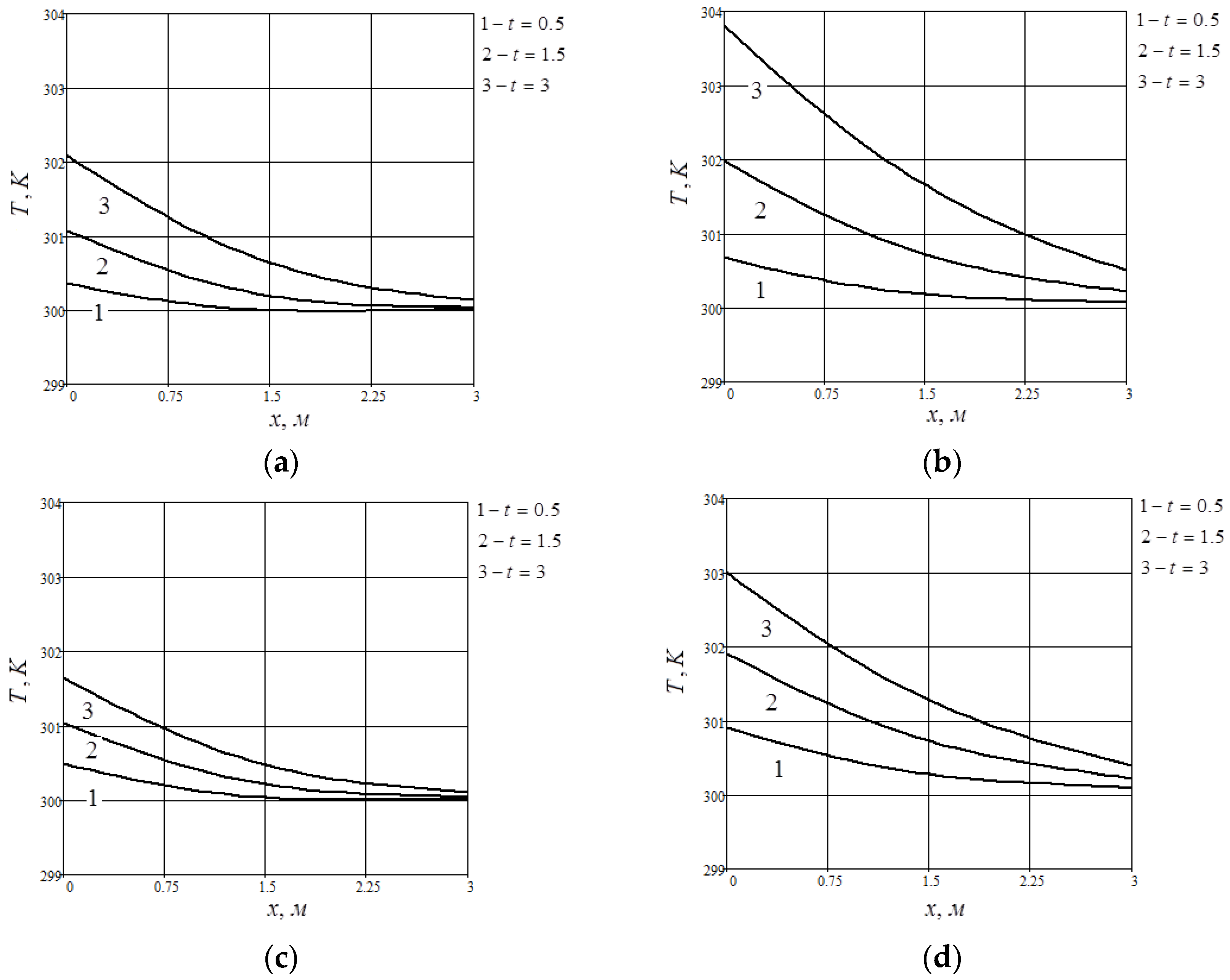
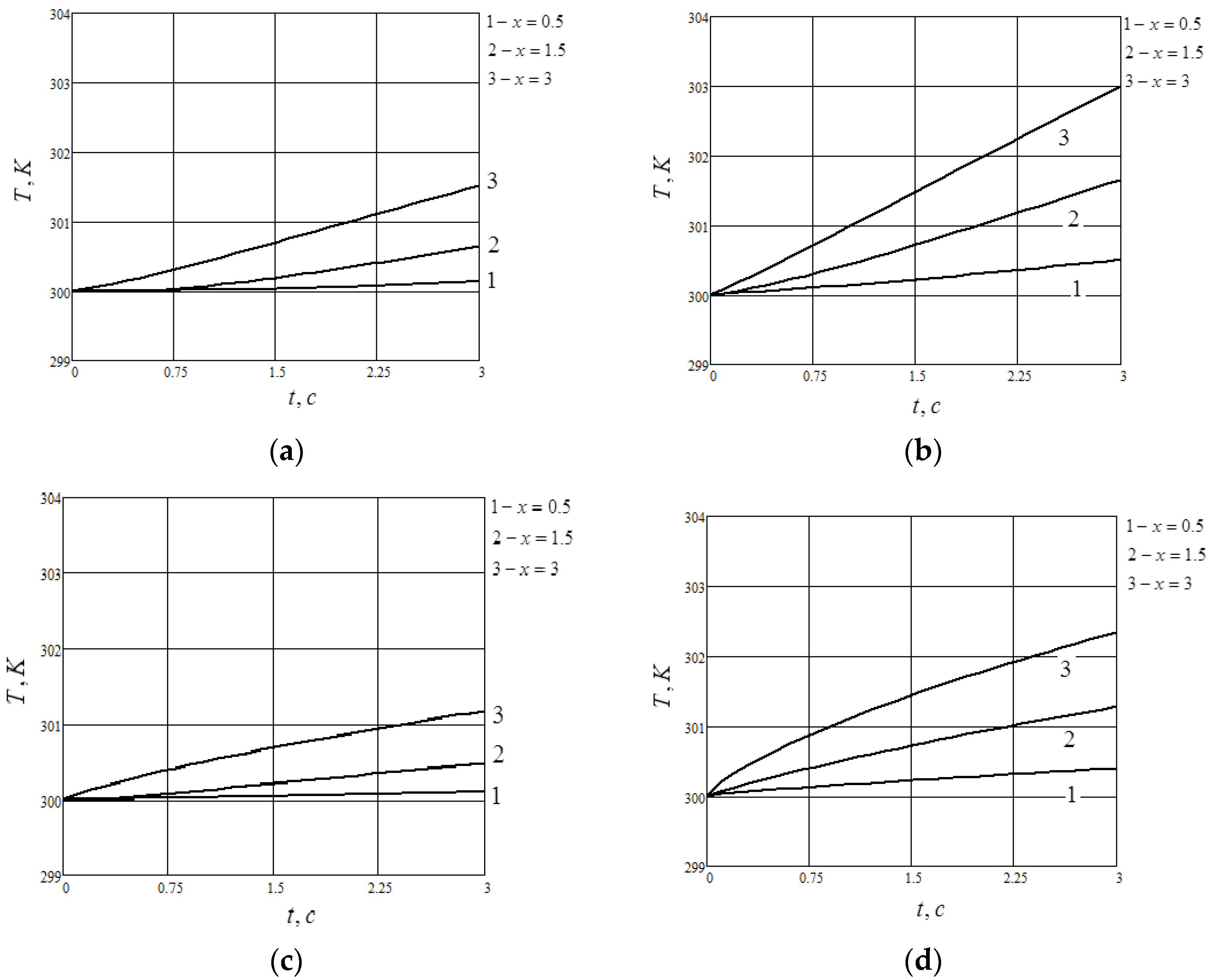
Figure 1 and
Figure 2 show graphs of solution (41) for various values of the fractional derivative parameters
α and
β.
As can be seen from
Figure 1 and
Figure 2, spatial correlations and memory effects have different influences on the final decision. With a decrease in the index of the spatial derivative (
β), an acceleration of the thermal conductivity processes is observed without a significant effect on the nature of the spatial and temporal dependences, while a decrease in the time derivative index (
α) leads to a significant slowdown of the processes while changing the nature of the nonlinearity of the time dependences.
6. Conclusions
We present a mathematical model of the thermal conductivity of a semi-infinite body that takes into account memory effects and spatial correlations. Graphs of the dependence of temperature on the spatial coordinate and time are constructed. When switching to a fractional time derivative, the heat transfer process slows down with a change in the nature of the time dependence. Thus, the transition to fractional derivatives makes it possible to study ultraslow heat transfer processes, which are typical for media with a fractal structure.
Author Contributions
Conceptualization, V.D.B. and A.A.A. (Abutrab A. Aliverdiev); Formal analysis, V.D.B., S.A.N., and A.A.A. (Anise A. Amirova); Investigation, V.D.B. and A.Z.Y.; Methodology, V.D.B. and A.Z.Y.; Project administration, V.D.B.; Resources, V.D.B. and A.A.A. (Abutrab A. Aliverdiev); Software, V.D.B.; Supervision, A.A.A. (Abutrab A. Aliverdiev); Validation, A.A.A. (Abutrab A. Aliverdiev), S.A.N., and A.A.A. (Anise A. Amirova); Visualization, V.D.B. and A.A.A. (Anise A. Amirova); Writing—original draft, V.D.B.; Writing—review & editing, A.A.A. (Abutrab A. Aliverdiev). All authors have read and agreed to the published version of the manuscript.
Funding
This research was carried out within the framework of the state assignments of the Ministry of Science and Higher Education of the Russian Federation with the partial support of the RFBR grant 20-08-00319a.
Institutional Review Board Statement
Not applicable.
Informed Consent Statement
Not applicable.
Data Availability Statement
Not applicable.
Conflicts of Interest
The authors declare no conflict of interest. The funders had no role in the design of the study; in the collection, analyses, or interpretation of data; in the writing of the manuscript; or in the decision to publish the results.
References
- Podlubny, I. Fractional Differential Equations: An Introduction to Fractional Derivatives, Fractional Differential Equations, to Methods of Their Solution and Some of Their Applications; Academic Press: San Diego, CA, USA, 1999; 340p. [Google Scholar]
- Uchaikin, V.V. Fractional Differentiation. In Fractional Derivatives for Physicists and Engineers. Nonlinear Physical Science; Uchaikin, V.V., Ed.; Springer: Berlin/Heidelberg, Germany, 2013; pp. 199–255. [Google Scholar] [CrossRef]
- Yu, L. Some uniqueness and existence results for the initial-boundary-value problems for the generalized time-fractional diffusion equation. Comput. Math. Appl. 2010, 59, 1766–1772. [Google Scholar] [CrossRef] [Green Version]
- Kemppainen, J.T. Existence and uniqueness of the solution for a time-fractional diffusion equation with Robin boundary condition. Abstr. Appl. Anal. 2011, 2011, 321903. [Google Scholar] [CrossRef] [Green Version]
- Zecová, M.; Terpák, J. Heat conduction modeling by using fractional-order derivatives. Appl. Math. Comput. 2015, 257, 365–373. [Google Scholar] [CrossRef] [Green Version]
- Beybalaev, V.D.; Abduragimov, E.I.; Yakubov, A.Z.; Meilanov, R.R.; Aliverdiev, A.A. Numerical research of non-isothermal filtration process in fractal medium with non-locality in time. Therm. Sci. 2021, 25, 465–475. [Google Scholar] [CrossRef] [Green Version]
- Zhou, Y. Basic Theory of Fractional Differential Equations; World Scientific: Hackensack, NJ, USA, 2014; 293p. [Google Scholar]
- Korchagina, A.N. Application of fractional order derivatives for solving problems of continuum mechanics. Izv. Altaj. Gos. Univ. [Izv. Altai State Univ. J.] 2014, 1, 65–67. [Google Scholar] [CrossRef]
- Uchaikin, V.V.; Sibatov, R.T. Fractional differential kinetics of dispersive transport as the consequence of its self-similarity. JETP Lett. 2007, 86, 512–516. [Google Scholar] [CrossRef]
- Kochubej, A.N. Diffusion of fractional order. Differ. Equ. 1990, 26, 485–492. [Google Scholar]
- Sierociuk, D.; Dzielinski, A.; Sarwas, G.; Petras, I.; Podlubny, I.; Skovranek, T. Modelling heat transfer in heterogeneous media using fractional calculus. Philos. Trans. R. Soc. A Math. Phys. Eng. Sci. 2013, 371, 20120146. [Google Scholar] [CrossRef] [PubMed] [Green Version]
- Povstenko, Y. Linear Fractional Diffusion-Wave Equation for Scientists and Engineers; Springer International Publishing: Berlin/Heidelberg, Germany, 2015. [Google Scholar] [CrossRef]
- Meilanov, R.P.; Shabanova, M.R. Peculiarities of solutions to the heat conduction equation in fractional derivatives. Tech. Phys. 2011, 56, 903–908. [Google Scholar] [CrossRef]
- Deng, S.; Ge, X. Local fractional Helmholtz simulation for heat conduction in fractal media. Thermal. Sci. 2019, 23, 1671–1675. [Google Scholar] [CrossRef] [Green Version]
- Zhmakin, A.I. Thermal conductivity beyond the Fourier law. Tech. Phys. 2021, 66, 1–22. [Google Scholar] [CrossRef]
- He, J.; Liu, F. Local Fractional Variational Iteration Method for Fractal Heat Transfer in Silk Cocoon Hierarchy. Nonlinear Sci. Lett. 2013, 4, 15. [Google Scholar]
| Disclaimer/Publisher’s Note: The statements, opinions and data contained in all publications are solely those of the individual author(s) and contributor(s) and not of MDPI and/or the editor(s). MDPI and/or the editor(s) disclaim responsibility for any injury to people or property resulting from any ideas, methods, instructions or products referred to in the content. |
© 2023 by the authors. Licensee MDPI, Basel, Switzerland. This article is an open access article distributed under the terms and conditions of the Creative Commons Attribution (CC BY) license (https://creativecommons.org/licenses/by/4.0/).


