Article

Refinable Trapezoidal Method on Riemann–Stieltjes Integral and Caputo Fractional Derivatives for Non-Smooth Functions

by
Gopalakrishnan Karnan
1 and
Chien-Chang Yen
2,*
1
The Graduate Institute of Applied Science and Engineering, Fu-Jen Catholic University, New Taipei City 242062, Taiwan
2
Department of Mathematics, Fu-Jen Catholic University, New Taipei City 242062, Taiwan
*
Author to whom correspondence should be addressed.
Fractal Fract. 2023, 7(3), 263; https://doi.org/10.3390/fractalfract7030263
Submission received: 6 February 2023 / Revised: 10 March 2023 / Accepted: 12 March 2023 / Published: 15 March 2023
(This article belongs to the Topic Fractional Calculus: Theory and Applications)

Abstract

:
The Caputo fractional α -derivative, 0 < α < 1 , for non-smooth functions with 1 + α regularity is calculated by numerical computation. Let I be an interval and D α ( I ) be the set of all functions f ( x ) which satisfy f ( x ) = f ( c ) + f ( c ) ( x a ) + g c ( x ) ( x c ) | ( x c ) | α , where x , c I and g c ( x ) is a continuous function for each c. We first extend the trapezoidal method on the set D α ( I ) and rewrite the integrand of the Caputo fractional integral as a product of two differentiable functions. In this approach, the non-smooth function and the singular kernel could have the same impact. The trapezoidal method using the Riemann–Stieltjes integral (TRSI) depends on the regularity of the two functions in the integrand. Numerical simulations demonstrated that the order of accuracy cannot be increased as the number of zones increases using the uniform discretization. However, for a fixed coarsest grid discretization, a refinable mesh approach was employed; the corresponding results show that the order of accuracy is k α , where k is a refinable scale. Meanwhile, the application of the product of two differentiable functions can also be applied to some Riemann–Liouville fractional differential equations. Finally, the stable numerical scheme is shown.

1. Introduction

Fractional calculus [1,2,3] has attracted increased interest over the last decade and has been applied in several fields including finance, control theory, electronic circuit theory, mechanics, physics, and signal processing [4,5,6,7,8,9,10,11]. There are two popular definitions of the fractional differentiation: the Riemann–Liouville derivative and the Caputo derivative. Let 0 < α < 1 , n be a positive integer with n 1 α < n , and a R .
  • Riemann–Liouville derivative: The Riemann–Liouville derivative of a function f ( x ) starting at the point a is
    a D t α f ( t ) = 1 Γ ( n α ) d n d t n a t f ( τ ) ( t τ ) α n + 1 d τ .
  • Caputo derivative: The Caputo derivative of a function f ( x ) starting at the point a is
    a C D t α f ( t ) = 1 Γ ( n α ) a t f ( n ) ( τ ) ( t τ ) α n + 1 d τ .
The comparison of these two definitions can be found in [12] and the definitions of fractional derivatives are also revised in some studies [11,12,13,14].
The trapezoidal rule was used for integration or differential equations in the following papers [15,16,17]. However, the functions of the integrand are assumed to be regular. This paper is devoted to the computation of the Caputo fractional derivative on financial derivatives [18,19,20,21]. In some of them, the functions of the stock or option prices are only of Lipschitz continuity. Our goal is to calculate the Caputo fractional integral for non-smooth functions. This calculation will also encounter the difficulty induced by the singular kernel. In [18], an implicit numerical discretization is used for the Riemann–Liouville integral to calculate the chaotic behavior for financial models. In [22], the treatment for a singular kernel involves the linear expansion of the smooth functions and direct integration of the product of the linear polynomial and the singular kernel. In our approach, we consider the function non-smooth. The function could be also singular, and the impact of the function for the integral is similar to the kernel.
Let n be a positive integer and [ a , b ] be an interval. Define h = ( b a ) / n and x i = a + i h , where i = 0 , 1 , 2 , , n . To explore the niche of this research, let us explain the following examples. The set of C k ( [ a , b ] ) represents the collection of all functions whose domain on [ a , b ] and they are of a continuous k-th derivative. If f C 2 ( [ a , b ] ) , it is well known in the textbook of numerical analysis, and the approximation is
a b f ( x ) d x = h 2 f ( a ) + f ( b ) + 2 j = 1 n 1 f ( x j ) ( b a ) 12 h 2 f ( ξ ) ,
where ξ is in ( a , b ) . For the particular case, f ( x ) = x a , the order of accuracy of the trapezoidal rule method is reduced because the function f ( x ) belongs exclusively to C 0 ( [ a , b ] ) .
Definition 1.
Let I be an interval and the set
D α ( I ) f : f ( x ) = f ( c ) + f ( c ) ( x c ) + g c ( x ) ( x c ) | x c | α ,
where g c ( x ) is a continuous function for each c I .
For example, I = [ 0 , 1 ] , α = 1 / 2 , and f ( x ) = x 3 / 2 . Then,
x 3 / 2 = c 3 / 2 + 3 2 c 1 / 2 ( x c ) + g c ( x ) ( x c ) | x c | 1 / 2
with
g c ( x ) = x 3 / 2 c 3 / 2 3 2 c 1 / 2 ( x c ) ( x c ) | x c | 1 / 2 , x c , 0 , x = c 0 .
If c = 0 , then g 0 ( 0 ) = 1 and g c ( x ) is continuous on [ 0 , 1 ] for each c [ 0 , 1 ] . Hence, x 3 / 2 D 1 / 2 ( [ 0 , 1 ] ) . Moreover, for a fixed x, the function h ( c ) = g c ( x ) may not be continuous on c since g 0 ( 0 ) = 1 and g c ( 0 ) = 1 / 2 for all c > 0 .
This paper is organized as follows. The order of accuracy for the trapezoidal method on the set D α ( I ) is derived in Section 2. The proposed method for calculation of Caputo fractional derivative is described in Section 3, using three examples. Smooth, regular and non-regular functions are used in numerical simulations in Section 4. Section 5 shows the analysis of the method to explain the obtained results and Section 6 demonstrates two applications of the proposed method. The conclusion is given in the last section.

2. Order of Accuracy for Trapezoidal Method on D α

In this section, we extend the analysis of the order of accuracy for the trapezoidal method on the set D α ( I ) . Let us begin to consider the interpolation on the set D α ( I ) .
Lemma 1.
Let f D α ( I ) . The linear interpolation of f on [ a , b ] I has the property
f ( x ) = f ( a ) b x b a + f ( b ) x a b a + h ( x ) b a ( x a ) ( b x ) ,
where h ( x ) is a continuous function and x [ a , b ] .
Proof. 
Since
f ( x ) = f ( a ) + f ( a ) ( x a ) + g a ( x ) ( x a ) | x a | α , f ( x ) = f ( b ) + f ( b ) ( x b ) + g b ( x ) ( x b ) | x b | α ,
we obtain
f ( x ) = f ( a ) b x b a + f ( b ) x a b a + 1 ( b a ) ( f ( a ) f ( b ) ) ( x a ) ( b x ) + 1 b a ( g a ( x ) | x a | α g b ( x ) | b x | α ) ( x a ) ( b x ) f ( a ) b x b a + f ( b ) x a b a + h ( x ) b a ( x a ) ( b x ) .
Here, h ( x ) = f ( a ) f ( b ) + g a ( x ) | x a | α g b ( x ) | b x | α . □
Lemma 2.
Let f D α ( I ) and [ a , b ] I . Then,
a b f ( x ) d x = 1 2 ( f ( a ) + f ( b ) ) ( b a ) + h ( ξ ) 6 ( b a ) 2 ,
where h ( ξ ) is a continuous function.
Proof. 
This lemma holds. It is followed by Lemma 1 and
a b f ( x ) d x = a b f ( a ) b x b a + f ( b ) x a b a + h ( x ) b a ( x a ) ( b x ) d x = 1 2 ( f ( a ) + f ( b ) ) ( b a ) + h ( ξ ) b a a b ( x a ) ( b x ) d x = 1 2 ( f ( a ) + f ( b ) ) ( b a ) + h ( ξ ) 6 ( b a ) 2 ,
where ξ in ( a , b ) , and the second equality is followed by the weighted mean value theorem. □
Lemma 3.
Let f D α ( I ) and [ a , b ] I . Then,
f ( b ) f ( a ) = ( g b ( a ) g a ( b ) ) | b a | α .
Proof. 
From the following,
f ( b ) f ( a ) b a = f ( a ) + g a ( b ) | b a | α , f ( a ) f ( b ) a b = f ( b ) + g b ( a ) | b a | α ,
and taking the subtraction of the above two equations, it yields
f ( b ) f ( a ) = ( g b ( a ) g a ( b ) ) | b a | α .
Moreover, g a ( x ) | x a | α g b ( x ) | b x | α ( | g a ( x ) | + | g b ( x ) | ) | b a | α for x [ a , b ] and | h ( x ) | ( | g b ( a ) g a ( b ) | + | g a ( x ) | + | g b ( x ) | ) | b a | α . Since h is continuous and bounded by the extremum theorem of continuous functions on a closed interval, Lemma 2 can be re-estimated to be Theorem 1 below.
Theorem 1.
Let f D α ( I ) and [ a , b ] I . Then,
a b f ( x ) d x = 1 2 ( f ( a ) + f ( b ) ) ( b a ) + O ( ( b a ) 2 + α ) .
Remark. 
If f C 2 ( I ) then g c = 1 2 f ( ξ ) , where ξ between c and x, then α = 1 .
Theorem 2.
Let f D α ( I ) and [ a , b ] I . If
f ( x ) = f ( c ) + f ( c ) ( x c ) + g c ( x ) ( x c ) | x c | α
and | g c ( a ) | is uniformly bounded for all c [ a , b ] , then
a b f ( x ) d x = 1 2 ( f ( a ) + f ( b ) ) ( b a ) + O ( ( b a ) 1 + α ) .
Proof. 
Using (3) as
f ( x ) f ( a ) = ( g x ( a ) g a ( x ) ) | x a | α ,
taking the integration of the above equation on [ a , b ] , we have
a b [ f ( x ) f ( a ) ] d x = a b ( g x ( a ) g a ( x ) ) | x a | α d x .
Since | g x ( a ) | is uniformly bounded for all x [ a , b ] and g a ( x ) is continuous on x [ a , b ] , it implies that | g x ( a ) g a ( x ) | is uniformly bounded for x [ a , b ] and
a b ( g x ( a ) g a ( x ) ) | x a | α d x = O ( a b ( x a ) α d x ) = O ( ( b a ) 1 + α ) .
Then,
a b f ( x ) d x = f ( a ) ( b a ) + a b [ f ( x ) f ( a ) ] d x = 1 2 ( f ( a ) + f ( b ) ) ( b a ) 1 2 ( f ( b ) f ( a ) ) ( b a ) + a b ( g x ( a ) g a ( x ) ) | x a | α d x = 1 2 ( f ( a ) + f ( b ) ) ( b a ) + O ( ( b a ) 1 + α ) .
The last equality is followed by 1 2 ( f ( b ) f ( a ) ) ( b a ) = 1 2 ( g b ( a ) g a ( b ) ) ( b a ) 1 + α and (4). Therefore, this theorem holds. □

3. Method

For the sake of simplicity and without loss generality, the case of n = 1 is considered in the whole paper. Equation (1) is equal to
a C D t α f ( t ) = 1 Γ ( 1 α ) a t f ( τ ) ( t τ ) α d τ ,
or
a C D t α f ( t ) = 1 Γ ( 1 α ) a t f ( τ ) φ ( t τ ) d τ ,
here, φ ( t ) = 1 1 α t 1 α .
Let the interval I = [ 0 , 1 ] and N be a positive integer. The interval I is divided into N-subintervals [ t 1 , t ] with the sample points t , = 1 , 2 , , N .
0 C D t α f ( t k ) = 1 Γ ( 1 α ) = 1 k t 1 t f ( τ ) φ ( t k τ ) d τ .
Since φ is monotonic whenever 0 < α < 1 , the inverse of φ exists. Using the substitution rule, y = φ ( t τ ) for fixed t, the integral
t 1 t f ( τ ) φ ( t k τ ) d τ
can be rewritten into
y 1 y f ( t k φ 1 ( y ) ) d y ,
where y 1 = φ ( t k t 1 ) and y = φ ( t k t ) . The linear interpolation of f ( y ) on the interval I with the endpoints φ ( t k t ) and φ ( t k t 1 ) is
f ( y ) = f ( t 1 ) y y y y 1 + f ( t ) y y 1 y y 1 .
Substituting (8) into (7), it yields
y 1 y f ( t k φ 1 ( y ) ) d y 1 2 ( f ( t 1 ) + f ( t ) ) ( y y 1 ) = 1 2 ( f ( t 1 ) + f ( t ) ) ( φ ( t k t ) φ ( t k t 1 ) ) .
The approximation in the last equation listed above represents the trapezoidal method but uses the Riemann–Stieltjes integral. The roles of f and g may be interchanged. Equation (9) is modified to
y 1 y f ( t k φ 1 ( y ) ) d y H 1 2 ( f ( t 1 ) + f ( t ) ) ( φ ( t k t ) φ ( t k t 1 ) ) + ( 1 H ) 1 2 ( f ( t ) f ( t 1 ) ) ( φ ( t k t ) + φ ( t k t 1 ) ) ,
where H = H ( | φ ( t k t ) φ ( t k t 1 ) | | f ( t ) f ( t ) | ) is the Heaviside step function. We refer to the approach in (10) as the TRSI method. If the function f is smooth and φ is non-smooth, then TRSI in (10) may only use H = 1 . On the other hand, the function φ is smooth and f is non-smooth, then TRSI in (10) may only use H = 0 . For Caputo fractional derivatives, φ is described as the form 1 1 α t 1 α and its derivative is singular at its origin. Therefore, if the function f is smooth, then H = 0 only occurs at the singularity of φ .
The stability of the TRSI method to use Equation (6) is to estimate the following:
| a C D t α f ( t k ) | 1 Γ ( 1 α ) = 1 k t 1 t f ( τ ) φ ( t k τ ) d τ 1 Γ ( 1 α ) = 1 k min { | φ ( t k t ) φ ( t k t 1 ) ) | , | f ( t ) f ( t 1 ) | } × 1 2 ( | f ( t 1 ) + f ( t ) | + | φ ( t k t ) + φ ( t k t 1 ) | ) .
If 1 Δ t min { | φ ( t k t ) φ ( t k t 1 ) ) | , | f ( t ) f ( t 1 ) | } is uniformly bounded for Δ t , 0 t | f ( s ) | d s and 0 t | φ ( s ) | d s are bounded, M , then
| a C D t α f ( t k ) | M Γ ( 1 α ) 0 t k | f ( s ) | d s + 0 t k | φ ( s ) | d s
and it follows that TRSI is stable. The condition 1 Δ t min { | φ ( t k t ) φ ( t k t 1 ) ) | , | f ( t ) f ( t 1 ) | } is uniformly bounded. It also indicates the existence of the Riemann–Stieltjes integral. It is identical to the existence of the Riemann–Stieltjes integral
a b f ( s ) d φ ( s ) ,
requires the condition that the discontinuity of f and φ cannot occur coincidentally, and vice versa. Therefore, the stability theorem of the TRSI method is stated in the following theorem.
Theorem 3.
The TRSI method is stable if the condition that the discontinuity of f and φ cannot occur coincidentally is held.

4. Simulations

Let us consider the interval I = [ 0 , 1 ] and there are N uniform cells; that is, each subinterval [ t 1 , t ] has the length Δ t = 1 N with the sample points t = N . We will vary N = 2 K from K = 5 to K = 12 . To probe the behavior of the TRSI method, let us define the 1-norm,2-norm and ∞-norm in vectors of numerical solutions by
f ( · ) 1 = = 1 N | f ( t ) | Δ t , f ( · ) 2 = ( = 1 N | f ( t ) | 2 ) 1 / 2 Δ t , f ( · ) = max 1 N | f ( t ) | .
Furthermore, the order of accuracy is defined as
O q , K = log 2 ( e K q e K + 1 q ) ,
where q = 1 , 2 , and e K is the error between the numerical and exact solutions at the size of zones 2 K . In the following subsection, we adopt three examples as model examples which represent the smooth, regular and non-smooth functions from Example 1 to Example 3 below, respectively.

4.1. Model Examples

Example 1.
Let us consider f ( t ) = 1 4 t 4 and g ( t ) = 2 t 1 2 . The polynomial is smooth because f ( n ) exists for any n, which is a non-negative integer. The Caputo fractional derivative of f ( t ) for α = 1 2 is
0 C D t α f ( t ) = 1 Γ ( 1 α ) 0 t f ( τ ) ( t τ ) α d τ = 1 Γ ( 1 2 ) 0 t τ 3 ( t τ ) 1 2 d τ .
The analytic solution is 0 C D t α f ( t ) = 32 35 π t 7 2 . The errors between the exact and numerical solutions are shown in Table 1, which demonstrates that the order of accuracy is near 1.5 for 1-norm, 2-norm and -norm.
Example 2.
Let us consider f ( t ) = 3 2 t 3 / 2 and g ( t ) = 2 t 1 2 . The power function f only can take the first derivate because f is singular at the origin. The Caputo fractional derivative of f ( t ) for α = 1 2 is
0 C D t α f ( t ) = 1 Γ ( 1 α ) 0 t f ( τ ) ( t τ ) α d τ = 1 Γ ( 1 2 ) , 0 t τ 1 2 ( t τ ) 1 2 d τ .
The analytic solution is 0 C D t α f ( t ) = π 2 t . The errors are shown in Table 2. The results demonstrate that the order of accuracy is near 1.5, 1.45 and 1 for 1-norm, 2-norm and -norm, respectively.
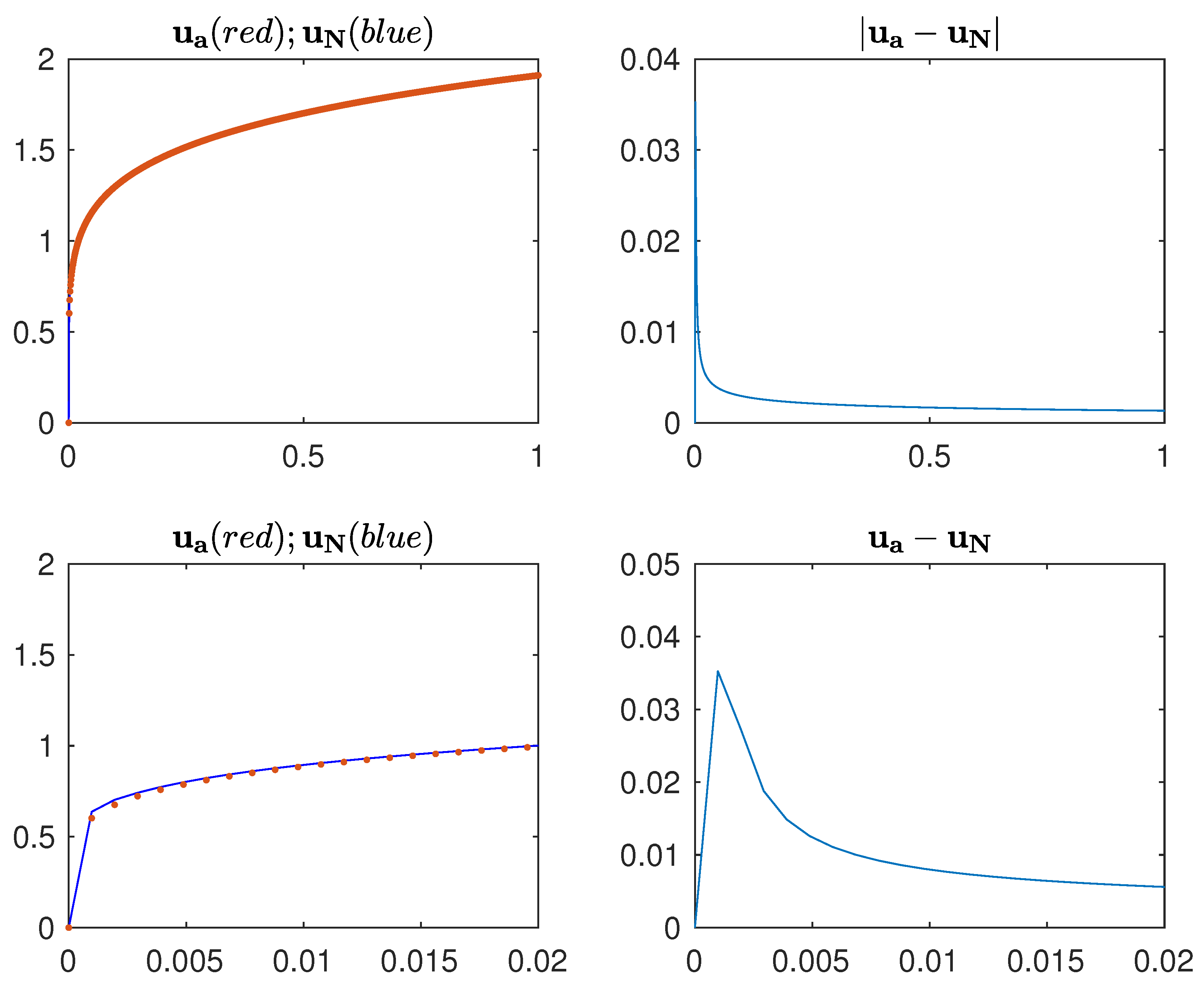
Example 3.
Let us consider f ( t ) = 2 t 1 / 2 and g ( t ) = 3 2 t 2 3 . The power function f does not have the first derivative because f ( 0 ) does not exist. The Caputo fractional derivative of f ( t ) for α = 1 3 is
0 C D t α f ( t ) = 1 Γ ( 1 α ) 0 t f ( τ ) ( t τ ) α d τ = 1 Γ ( 2 3 ) 0 t τ 1 2 ( t τ ) 1 3 d τ .
The analytic solution is 0 C D t α f ( t ) = Γ ( 1 2 ) Γ ( 7 6 ) t 1 6 . The errors are shown in Table 3. The order of accuracy is near 0.52, 0.54 and 0.16 for 1-norm, 2-norm and -norm, respectively. In Figure 1, the top-left panel shows the exact solution (red dot line) and the numerical solution (blue solid line). The errors between the numerical and exact solutions are shown in the top-right panel. The zoom-in profiles on [ 0 , 0.2 ] are shown in the corresponding panels below.
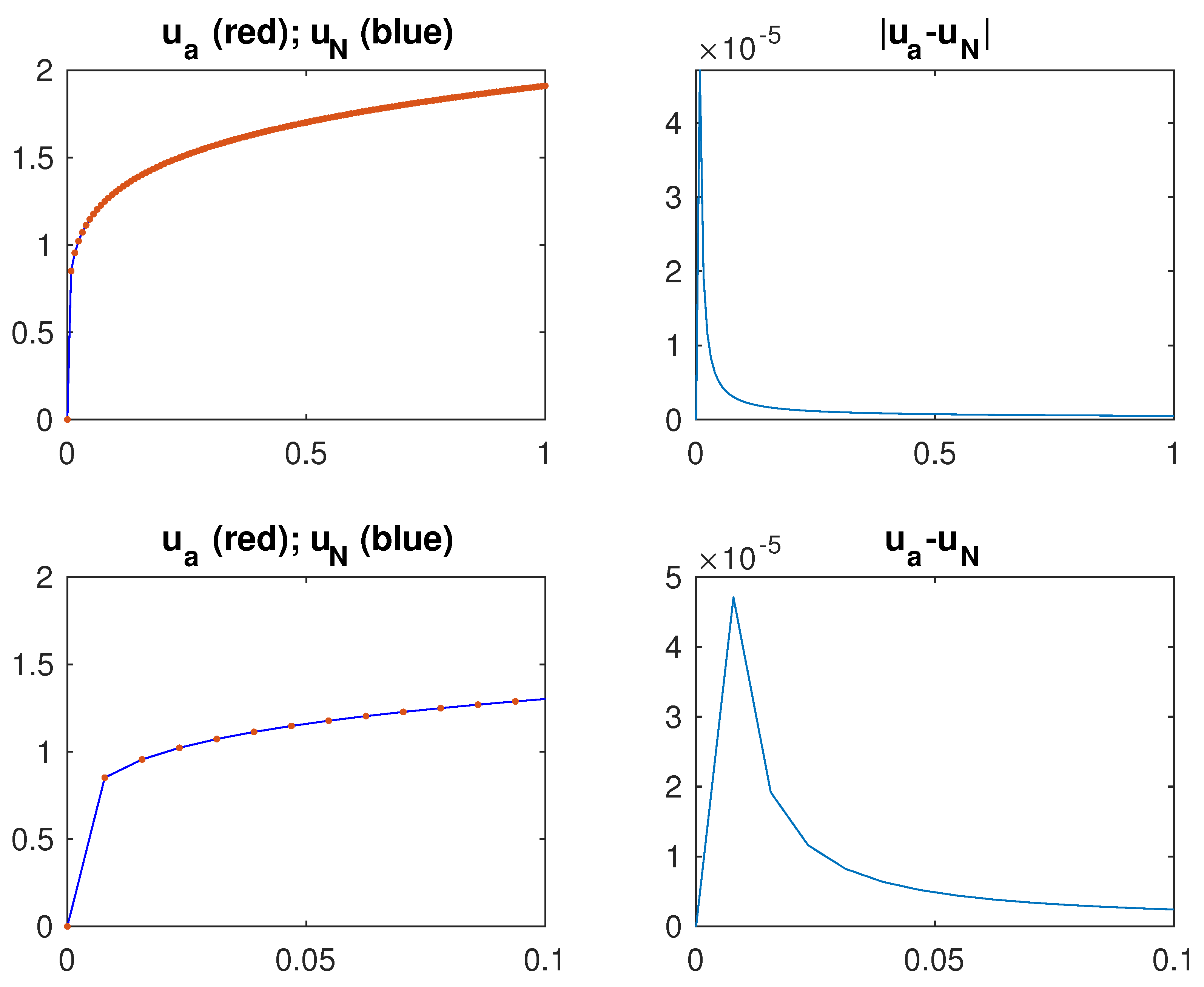
The approximation of the non-smooth or continuous function may improve the accuracy by refining the meshes. However, it is not equivalent to a finer mesh refinement in this case, as the kernel function φ ( t k s ) is not only non-smooth, but it is singular for fixed t k . Therefore, we divide the subinterval by K -zones again. More precisely,
t 1 t f ( s ) ( t k s ) α d s = m = 1 K t , m 1 t , m f ( s ) φ ( t k s ) d s ,
where t , m = t 1 + m Δ K , m = 0 , 1 , 2 , , K , with Δ K = t t 1 K . The results of fixed N = 128 for K = 2 p , p = 2 , 3 , , 6 are shown in Table 4 and the corresponding profiles are shown in Figure 2. The errors were reduced from 2.8 × 10 2 to 4.7 × 10 5 ; see Table 3 and Table 4, respectively.

4.2. A Comparison Study

The modified trapezoidal rule (MTR) [22] uses the linear interpolation on f ( s ) rather than f ( s ) ( t k s ) α in the traditional sense for the following integral, and we rewrite it as shown below. The integral can be approximated by
t 1 t f ( s ) ( t k s ) α d s f ( t 1 ) t t 1 W L , k + f ( t ) t t 1 W R , k ,
where
W L , k = ( t k t ) 2 α 1 α ( t k t ) ( t k t 1 ) 1 α 1 α ( t k t ) 2 α 2 α + ( t k t 1 ) 2 α 2 α , W R , k = ( t k t ) 2 α 2 α ( t k t 1 ) 2 α 2 α ( t k t 1 ) ( t k t ) 1 α 1 α + ( t k t 1 ) ( t k t 1 ) 1 α 1 α .
The errors are shown in Table 5 and Table 6 for model example 1 and 2, respectively. However, Example 3 cannot be simulated by the MTR method because the derivative of the exact function does not exist at the origin.

5. Error Analysis

Let us start to observe the approximation of the function y = t by the linear interpolation L ( t ) on [ t 1 , t ] ,
L ( t ) = t t 1 t t 1 ( t t 1 ) + t 1 .
The error e ( t ) = y ( t ) L ( t ) on [ t 1 t ] has the maximum error
| e ( t * ) | = | ( t t 1 ) 2 4 ( t + t 1 ) 2 | ,
where t * = 1 4 ( t + t 1 ) 2 . Let t = Δ t , = 0 , 1 , , N ; the error for = 1 is 1 4 Δ t . This explains that the reason for Example 2 using the trapezoidal method is only of first-order accuracy.
Theorem 4.
Let the function L ( t ) be the linear interpolation of the function f ( t ) on each subinterval [ t 1 , t ] , = 1 , 2 , , N and 0 t | φ ( t τ ) | d τ is uniformly bounded for 0 t 1 . The modified trapezoidal rule for calculation
0 C D t α f ( t ) = 1 Γ ( 1 α ) 0 t f ( τ ) ( t τ ) α d τ
has the error bounded by C max { | L ( t ) f ( t ) | } and
C = 1 Γ ( 1 α ) 0 t | t τ | d τ .
Proof. 
The error is given by
| 1 Γ ( 1 α ) 0 t f ( τ ) ( t τ ) α d τ 1 Γ ( 1 α ) 0 t L ( τ ) ( t τ ) α d τ | .
It follows that the error is less than
1 Γ ( 1 α ) 0 t | f ( τ ) L ( τ ) | ( t τ ) α d τ 1 Γ ( 1 α ) 0 t max | f ( τ ) L ( τ ) ( t τ ) | α d τ = max | f ( τ ) L ( τ ) | 1 Γ ( 1 α ) 0 t | t τ | α d τ
Theorem 4 can be applied to explain the results (Table 5 and Table 6) for Example 1 and Example 2 obtained using MTR. Next, we will analyze the TRSI method. Let us first recall the error analysis for smooth functions as Theorem 5 below for the trapezoidal method in comparison with the estimation of the errors for the functions in D α ( I ) shown in Theorem 6 below.
Let
H ( t ) = t 1 t f ( s ) g ( t k s ) d s
and Δ t = ( t t 1 ) . Then,
H ( t ) = H ( t 1 ) + H ( t 1 ) ( Δ t ) + 1 2 H ( t 1 ) ( Δ t ) 2 + O ( ( Δ t ) 3 )
if H has the third continuous derivative. Furthermore, if f and g are continuous whenever < N , then
f ( t ) = f ( t 1 ) + 1 2 f ( t 1 ) ( Δ t ) + O ( ( Δ t ) 2 ) , g ( t k t ) = g ( t k t 1 ) 1 2 g ( t k t 1 ) ( Δ t ) + O ( ( Δ t ) 2 ) .
It follows that
t 1 t f ( s ) g ( t k s ) d s = 1 2 ( f ( t 1 ) + f ( t ) ) ( g ( t k t ) g ( t k t 1 ) ) + O ( ( Δ t ) 3 ) .
The above approximation leads to the theorem below.
Theorem 5.
If f exists and is continuous and g ( t ) = t 1 α 1 α , 0 < α < 1 then
t 1 t f ( s ) g ( t k s ) d s = 1 2 ( f ( t 1 ) + f ( t ) ) ( g ( t k t ) g ( t k t 1 ) ) + O ( ( Δ t ) 3 )
for < k . Furthermore,
= 1 k 1 t 1 t f ( s ) g ( t k s ) d s = = 1 k 1 1 2 ( f ( t 1 ) + f ( t ) ) ( g ( t k t ) g ( t k t 1 ) ) + O ( ( Δ t ) 2 )
and for = k , the following approximation is reduced to
t k 1 t k f ( s ) g ( t k s ) d s = 1 2 ( f ( t k ) + f ( t k 1 ) ) ( g ( t k t k ) g ( t k t k 1 ) ) + O ( Δ t ) .
From (7) and Theorem 2, if f D α ( I ) , then we have
y 1 y f ( t k φ 1 ( y ) ) d y = 1 2 f ( t 1 ) + f ( t ) ( y y 1 ) + O ( ( y y 1 ) 1 + α )
for < k and for = k , it is reduced to
y 1 y f ( t k φ 1 ( y ) ) d y = 1 2 f ( t 1 ) + f ( t ) ( y y 1 ) + O ( ( y y 1 ) α ) .
Furthermore, the term O ( ( y y 1 ) 1 + α ) = O ( ( t t 1 ) 1 + α ) . On the other hand,
y 1 y f ( t k φ 1 ( y ) ) d y = 1 2 ( f ( t ) f ( t 1 ) ) ( φ ( t k t ) + φ ( t k t 1 ) ) + O ( ( f ( t ) f ( t 1 ) ) 3 ) = 1 2 ( f ( t ) f ( t 1 ) ) ( φ ( t k t ) + φ ( t k t 1 ) ) + O ( ( t t 1 ) 3 )
Theorem 6.
If f D α ( I ) and g ( t ) = t 1 α 1 α , 0 < α < 1 then
t 1 t f ( s ) g ( t k s ) d s = 1 2 ( f ( t 1 ) + f ( t ) ) ( g ( t k t ) g ( t k t 1 ) ) + O ( ( Δ t ) 1 + α )
for < k . Furthermore,
= 1 k 1 t 1 t f ( s ) g ( t k s ) d s = = 1 k 1 1 2 ( f ( t 1 ) + f ( t ) ) ( g ( t k t ) g ( t k t 1 ) ) + O ( ( Δ t ) α )
and for = k , the following approximation is reduced to
t k 1 t k f ( s ) g ( t k s ) d s = 1 2 ( f ( t k ) + f ( t k 1 ) ) ( g ( t k t k ) g ( t k t k 1 ) ) + O ( ( Δ t ) α ) .
Let k be a positive integer and 0 < α < 1 . If an integration scheme has the order of accuracy α ,
a b f ( s ) g ( b s ) d s = N ( h j ) + O ( h j α ) ,
where h j = ( b a ) / 2 j and N for some numerical method, then the refinable approach using the mesh h j + k is read as
a b f ( s ) g ( b s ) d s = N ( h j + k ) + O ( h k + j α ) .
This implies that the order of accuracy is log 2 ( h j α / h k + j α ) = log 2 ( 2 k α ) = k α .

6. Applications

We are going to demonstrate the applications of the integrand in (10) rewritten as a product of two derivatives of functions on fractional differential equations with Caputo and Riemann–Liouville derivatives.

6.1. Fractional Differential Equation with Caputo Derivatives

We first solve the fractional differential equation to evaluate the TRSI method
IVP : 0 C D t α y + y = 3 4 t π + t 3 / 2 y ( 0 ) = y ( 0 ) = 0
The exact solution for (14) is y ( t ) = t 3 / 2 .
The discretization approach at the zone [ t 1 , t ] is
1 Γ ( 1 α ) m = 1 t m 1 t m y ( s ) ( t s ) α d s + y ( t ) = 3 4 t π + ( t ) 3 / 2 .
If y ( t m ) and y ( t m ) for m = 0 , 1 , , 1 are given, then we have to solve y ( t ) and y ( t ) . There are two unknowns, y ( t ) and y ( t ) , in Equation (14) but only one equation. We further impose the condition
y ( t ) y ( t 1 ) Δ t = y ( t ) + y ( t 1 ) 2 ,
which means that the central difference at the midpoint of t and t approximation. It gives us
Δ t 2 y ( t ) y ( t ) = Δ t 2 y ( t 1 ) y ( t 1 ) .
Coupling (14) and (15), the linear system for y ( t ) and y ( t ) is obtained
a 11 a 12 a 21 a 22 y ( t ) y ( t ) = b 1 b 2 ,
where a 12 = 1 , a 22 = 1 , a 21 = Δ t 2 ,
a 11 = 1 Γ ( 1 α ) ( φ ( Δ t ) ) , b 1 = 3 4 t π + ( t ) 3 / 2 + φ ( Δ t ) 2 Γ ( 1 α ) 1 Γ ( 1 α ) m = 1 1 1 2 ( y ( t m ) + y ( t m 1 ) ) ( φ ( t t m ) φ ( t t m 1 ) ) .
The errors between the analytic and numerical solutions for the IVP problem are shown in Table 7. It shows the order of accuracy is 1.49 for the 1-norm and 2-norm and 1.46 for the -norm.

6.2. Fractional Differential Equation with Riemann–Liouville Derivatives

In this subsection, we consider the fractional ordinary equation [23]:
IVP 2 : d d t 1 Γ ( 1 α ) 0 t y ( s ) ( t s ) α + y ( t ) = 3 4 π + t 3 / 2 y ( 0 ) = y ( 0 ) = 0
The exact solution is the same as the previous case, y ( t ) = t 3 / 2 . Taking the integration from t 0 = 0 to t , we obtain
1 Γ ( 1 α ) 0 t y ( s ) ( t s ) α d s + 0 t y ( t ) d t = 3 4 t π + 2 5 ( t ) 5 / 2
or
1 Γ ( 1 α ) m = 1 t m 1 t m y ( s ) ( t s ) α d s + 0 t y ( t ) d t = 3 4 t π + 2 5 ( t ) 5 / 2 .
We use the traditional trapezoidal method for the second integral on the left-hand side as the same approach in [23]. Meanwhile, people can define the coefficients a ˜ 11 = a 11 , a ˜ 21 = a 21 , b ˜ 2 = b 2 and
a ˜ 12 = 1 2 Δ t , b ˜ 1 = b 1 1 2 m = 1 1 ( y ( t m ) + y ( t m 1 ) ) Δ t ,
where a 11 , a 12 , a 21 , a 22 , b 1 , and b 2 are defined in the (Section 6.1). The numerical solution is obtained by solving the following linear system:
a ˜ 11 a ˜ 12 a ˜ 21 a ˜ 22 y ( t ) y ( t ) = b ˜ 1 b ˜ 2 .
The errors between the exact and numerical solutions are shown in Table 8, which demonstrates that the order of accuracy is near 1.49 for 1-norm and 2-norm and 1.48 for -norm.

7. Conclusions

The analysis of the trapezoidal method was extended from C 2 to D α ( I ) and, for each f D α ( I ) , has the order of accuracy 1 + α . The trapezoidal method using the Riemann–Stieltjes integral on Caputo fractional derivatives for non-smooth functions was proposed, and the approximation ability was also investigated using three models of examples of smoothness, regularity and non-smoothness. The product of the integrand reveals that, if f D α ( I ) and the integration is approximated by using the differential d f , then the trapezoidal method has the second order of accuracy compared to the traditional one. On the other hand, if the integration is approximated by using the differential d φ , φ ( x ) = 1 1 α x 1 α , then the order of accuracy for the trapezoidal method is of the α fractional order of accuracy. The novelty of this method can be addressed to automatically choose the non-smooth functions or the singular kernel for linear interpolation.
The errors in Table 3 show that increasing the number of zones cannot significantly improve the accuracy, and the order of accuracy is 0.16 for -norm. Therefore, a refining mesh shown in Table 4 demonstrated that the order of accuracy is 1.59 for the -norm. To confirm this point, we further apply the refinable approach to MTR. The result for the MTR method using a refinable approach is shown in Table 9; the order of accuracy improves from 1.0 to 1.50 for the -norm, see Table 6 and Table 9.

Author Contributions

Conceptualization, G.K. and C.-C.Y.; methodology, C.-C.Y.; formal analysis, C.-C.Y.; investigation, G.K.; writing—original draft preparation, G.K.; writing—review and editing, C.-C.Y. All authors have read and agreed to the published version of the manuscript.

Funding

C.C. Yen acknowledges the grant support from the Ministry of Science and Technology (MoST) under 109-2115-M-030-004-MY2 and National Science and Technology Council (NSC) under 111-2115-M-030-002.

Informed Consent Statement

Not applicable.

Data Availability Statement

Not applicable.

Acknowledgments

We sincerely appreciate the reviewers for all valuable comments and suggestions that helped us to improve the quality and the better presentation of the results in the manuscript.

Conflicts of Interest

The authors declare no conflict of interest.

References

  1. Kilbas, A.A.; Srivastava, H.M.; Trujillo, J.J. Theory and Applications of Fractional Differential Equations; Series North-Holland Mathematics Studies; North-Holland: New York, NY, USA, 2006. [Google Scholar]
  2. Oldham, K.; Spanier, J. The Fractional Calculus, Theory and Applications of Differentiation and Integration of Arbitrary Order; Academic Press: Cambridge, MA, USA, 1974. [Google Scholar]
  3. Podlubny, I. Fractional Differential Equations; Academic Press: Cambridge, MA, USA, 1999. [Google Scholar]
  4. Burrage, K.; Hale, N.; Kay, D. An efficient implicit FEM scheme for fractional-in-space reaction-diffusion equations. SIAM J. Sci. Comput. 2012, 34, A2145–A2172. [Google Scholar] [CrossRef] [Green Version]
  5. Cafagna, D.; Grassi, G. Observe-based projective synchronization of fractional systems via a scalar signal: Application to hyperchaotic Rössler systems. Nonlinear Dyn. 2012, 68, 117–128. [Google Scholar] [CrossRef]
  6. Caponetto, R.; Maione, G.; Pisano, A.; Rapaić, M.M.R.; Usai, E. Analysis and shaping of the self-sustained oscillations in relay controlled fractional-order systems. Fract. Calc. Appl. Anal. 2013, 16, 93–108. [Google Scholar] [CrossRef]
  7. Diethelm, K. An investigation of some nonclassical methods for the numerical approximation of Caputo-type fractional Derivatives. Numer. Algorithms 2008, 47, 361–390. [Google Scholar] [CrossRef]
  8. Garrappa, R.; Poplizio, M. On accurate product integration rules for linear fractional differential equations. J. Comput. Appl. Math. 2011, 235, 1085–1097. [Google Scholar] [CrossRef]
  9. Miller, K.S. An Introduction to Fractional Calculus and Fractional Differential Equations; John Wiley and Sons: New York, NY, USA, 1993. [Google Scholar]
  10. Moret, I.; Novati, P. On the convergence of Krylov subspace methods for matrix Mittag-Leffler functions. SIAM. J. Numer. Anal. 2011, 49, 2144–2164. [Google Scholar] [CrossRef]
  11. Rahimy, M. Applications of fractional differential equations. Appl. Math. Sci. 2010, 4, 2453–2461. [Google Scholar]
  12. Khalil, R.; Horani, M.A.I.; Yousef, A.; Sabaheh, M. A new definition of fractional derivative. J. Comput. Appl. Math. 2014, 264, 65–70. [Google Scholar] [CrossRef]
  13. Garrappa, R. Trapezoidal methods for fractional differential equations: Theoretical and computational aspects. Math. Comput. Simul. 2015, 10, 96–112. [Google Scholar] [CrossRef] [Green Version]
  14. Pandiangan, N.; Johar, D.; Purwani, S. Fractional integral approximation and Caputo derivatives with modification of trapezoidal rule. World Sci. News 2021, 153, 169–180. [Google Scholar]
  15. Arashad, S.; Huang, J.; Khaliq, A.Q.M.; Tang, Y. Trapezoid scheme for time-space fractional diffusion equation with Riesz derivative. J. Comput. Phys. 2017, 350, 1–15. [Google Scholar] [CrossRef]
  16. Odibat, Z. Approximations of fractional integrals and Caputo fractional derivatives. Appl. Math. Comput. 2006, 178, 527–533. [Google Scholar] [CrossRef]
  17. Rapaić, M.R.; Pisano, A.; Jeličić, Z.D.J. Trapezoidal rule for numerical evaluation of fractional order integrals with applications to simulation and identification of fractional order system. In Proceedings of the 2012 IEEE International Conference on Control Applications (CCA), Part of 2012 IEEE Multi-Conference on Systems and Control, Dubrovnik, Croatia, 3–5 October 2012. [Google Scholar]
  18. Diouf, M.; Sene, N. Analysis of the financial chaotic model with the fractional derivative operator. Complexity 2020, 2020, 9845031. [Google Scholar] [CrossRef]
  19. Fall, A.N.; Ndiaye, S.N.; Sene, N. Black-Scholes option pricing equations described by the Caputo generalized fractional derivative. Chaos Solitons Fractals 2019, 125, 108–118. [Google Scholar] [CrossRef]
  20. Jumaric, G. New stochastic fractional models of the Malthusian growth the poissonian birth process and optimal management of population. Math. Comput. Model 2006, 44, 231–254. [Google Scholar] [CrossRef]
  21. Ma, S.; Xu, Y.; Yue, W. Numerical solutions of a variable-order fractional financial system. J. Appl. Math. 2012, 2012, 417942. [Google Scholar] [CrossRef] [Green Version]
  22. Jahanshahi, S.; Babolian, E.; Torres, D.F.M.; Vahidi, A. A fractional Gauss-Jacobi quadrature rule for approximating fractional integrals and derivatives. Chaos Solitons Fractals 2017, 102, 295–304. [Google Scholar] [CrossRef] [Green Version]
  23. Li, B.; Wang, T.; Xie, X. Analysis of the L1 scheme for fractional wave equations with nonsmooth data. Comput. Math. Appl. 2021, 90, 1–12. [Google Scholar] [CrossRef]
Figure 1. The profiles of the simulations of Example 3. The analytic ( u a ) and the numerical u N solutions are shown in the top-left panel. The absolute value of the error | u a u N | is shown in the top-right panel. The zoom-in profiles on [ 0 , 0.2 ] are shown in the corresponding panels below.
Fractalfract 07 00263 g001
Figure 2. The profiles of the simulations of Example 3 with a refinable approach. The analytic ( u a ) and the numerical u N solutions are in the top-left panel. The absolute value of the error | u a u N | is in the top-right panel. The zoom-in profiles on [ 0 , 0.2 ] are shown in the corresponding panels below.
Fractalfract 07 00263 g002
Table 1. The errors between numerical and analytic solutions for f ( t ) = 1 4 t 4 and the order of accuracy. The order of accuracy is near 1.5 for 1-norm, 2-norm and -norm.
N E 1 E 2 E N / N + 1 O 1 O 2 O
32 1.038 × 10 3 1.415 × 10 3 3.124 × 10 3 32 / 64 1.411.411.40
64 3.915 × 10 4 5.312 × 10 4 1.186 × 10 3 64 / 128 1.431.441.43
128 1.449 × 10 4 1.960 × 10 4 4.391 × 10 4 128 / 256 1.451.461.46
256 5.291 × 10 5 7.140 × 10 5 1.602 × 10 4 256 / 512 1.471.471.47
512 1.914 × 10 5 2.579 × 10 5 5.784 × 10 5 512 / 1024 1.481.481.48
1024 6.880 × 10 6 9.256 × 10 6 2.075 × 10 5 1024 / 2048 1.481.481.49
2048 2.461 × 10 6 3.308 × 10 6 7.413 × 10 6 2048 / 4096 1.491.491.49
4096 8.771 × 10 7 1.179 × 10 6 2.639 × 10 6 ----
Table 2. The errors between numerical and analytic solutions for f ( t ) = 2 3 t 3 / 2 and the order of accuracy. The order of accuracy is near 0.52, 0.54 and 0.16 for 1-norm, 2-norm and -norm, respectively.
N E 1 E 2 E N / N + 1 O 1 O 2 O
32 2.390 × 10 3 2.920 × 10 3 1.006 × 10 2 32 / 64 1.471.411.00
64 8.649 × 10 4 1.100 × 10 3 5.032 × 10 3 64 / 128 1.481.421.00
128 3.109 × 10 4 4.115 × 10 4 2.516 × 10 3 128 / 256 1.481.421.00
256 1.112 × 10 4 1.531 × 10 4 1.258 × 10 3 256 / 512 1.491.431.00
512 3.967 × 10 5 5.668 × 10 5 6.290 × 10 4 512 / 1024 1.491.441.00
1024 1.411 × 10 5 2.091 × 10 5 3.145 × 10 4 1024 / 2048 1.491.441.00
2048 5.001 × 10 6 7.686 × 10 6 1.572 × 10 4 2048 / 4096 1.501.451.00
4096 1.777 × 10 6 2.818 × 10 6 7.862 × 10 4 ----
Table 3. The errors between numerical and analytic solutions for f ( t ) = 2 t 1 / 2 and the order of accuracy. It shows that the order of accuracy is near 0.52, 0.54 and 0.16 for 1-norm, 2-norm and -norm, respectively.
N E 1 E 2 E N / N + 1 O 1 O 2 O
32 1.565 × 10 2 1.967 × 10 2 6.281 × 10 2 32 / 64 0.630.580.16
64 1.009 × 10 2 1.315 × 10 2 5.596 × 10 2 64 / 128 0.610.580.16
128 6.635 × 10 3 8.825 × 10 3 4.985 × 10 2 128 / 256 0.580.570.16
256 4.445 × 10 3 5.948 × 10 3 4.441 × 10 2 256 / 512 0.550.560.16
512 3.029 × 10 3 4.031 × 10 3 3.957 × 10 2 512 / 1024 0.540.550.16
1024 2.087 × 10 3 2.746 × 10 3 3.525 × 10 2 1024 / 2048 0.520.550.16
2048 1.451 × 10 3 1.881 × 10 3 3.140 × 10 2 2048 / 4096 0.520.540.16
4096 1.014 × 10 3 1.294 × 10 3 2.780 × 10 2 ----
Table 4. The errors between numerical and analytic solutions for f ( t ) = 2 t 1 / 2 and the order of accuracy using TRSI with refining mesh. The order of accuracy is near 1.76, 1.61 and 1.59 for 1-norm, 2-norm and -norm, respectively.
K ( N = 128 ) E 1 E 2 E K p 1 / K p O 1 O 2 O
4 9.393 × 10 4 1.651 × 10 3 1.399 × 10 2 4 / 8 1.881.761.72
8 2.548 × 10 4 4.860 × 10 4 4.260 × 10 3 8 / 16 1.861.721.67
16 7.013 × 10 5 1.480 × 10 4 1.343 × 10 3 16 / 32 1.831.671.63
32 1.973 × 10 5 4.636 × 10 5 4.328 × 10 4 32 / 64 1.801.641.60
64 5.690 × 10 6 1.487 × 10 5 1.418 × 10 4 64 / 128 1.761.611.59
128 1.685 × 10 6 4.861 × 10 6 4.708 × 10 5 ----
Table 5. The errors between numerical and analytic solutions for f ( t ) = 1 4 t 4 and the order of accuracy using the MTR method. It shows that the order of accuracy is 2.0 for 1-norm, 2-norm and -norm.
N E 1 E 2 E N / N + 1 O 1 O 2 O
32 1.423 × 10 4 1.776 × 10 4 3.473 × 10 4 32 / 64 2.001.991.98
64 3.565 × 10 5 4.459 × 10 5 8.830 × 10 5 64 / 128 1.991.991.98
128 8.958 × 10 6 1.121 × 10 5 2.233 × 10 5 128 / 256 1.991.991.98
256 2.252 × 10 6 2.818 × 10 6 5.629 × 10 6 256 / 512 1.991.991.99
512 5.656 × 10 7 7.077 × 10 7 1.415 × 10 6 512 / 1024 1.991.991.99
1024 1.419 × 10 7 1.776 × 10 7 3.553 × 10 7 1024 / 2048 2.002.002.00
2048 3.559 × 10 8 4.451 × 10 8 8.907 × 10 8 2048 / 4096 2.002.002.00
4096 8.917 × 10 9 1.115 × 10 8 2.231 × 10 8 ----
Table 6. The errors between numerical and analytic solutions for f ( t ) = 2 3 t 3 / 2 and the order of accuracy. It shows that the order of accuracy is near 1.49, 1.44 and 1.0 for 1-norm, 2-norm and -norm, respectively.
N E 1 E 2 E N / N + 1 O 1 O 2 O
32 1.161 × 10 3 1.362 × 10 3 4.187 × 10 3 32 / 64 1.451.401.00
64 4.237 × 10 4 5.176 × 10 4 2.093 × 10 3 64 / 128 1.471.411.00
128 1.533 × 10 4 1.950 × 10 4 1.047 × 10 3 128 / 256 1.481.421.00
256 5.507 × 10 5 7.293 × 10 5 5.233 × 10 4 256 / 512 1.481.431.00
512 1.969 × 10 5 2.713 × 10 5 2.617 × 10 4 512 / 1024 1.491.431.00
1024 7.019 × 10 6 1.004 × 10 5 1.308 × 10 4 1024 / 2048 1.491.441.00
2048 2.496 × 10 6 3.703 × 10 6 6.542 × 10 5 2048 / 4096 1.491.441.00
4096 8.861 × 10 6 1.361 × 10 6 3.271 × 10 5 ----
Table 7. The errors between the analytic and numerical solutions for the IVP problem are shown in this table. The order of accuracy is 1.49 for 1-norm and 2-norm and 1.46 for -norm.
N E 1 E 2 E N / N + 1 O 1 O 2 O
32 8.440 × 10 4 8.490 × 10 4 1.000 × 10 3 32 / 64 1.451.441.38
64 3.094 × 10 4 3.121 × 10 4 3.847 × 10 4 64 / 128 1.461.461.40
128 1.123 × 10 4 1.135 × 10 4 1.461 × 10 4 128 / 256 1.471.471.41
256 4.045 × 10 5 4.097 × 10 5 5.486 × 10 5 256 / 512 1.481.481.43
512 1.449 × 10 5 1.470 × 10 5 2.041 × 10 5 512 / 1024 1.491.481.44
1024 5.172 × 10 6 5.254 × 10 6 7.536 × 10 6 1024 / 2048 1.491.491.45
2048 1.841 × 10 6 1.872 × 10 6 2.764 × 10 6 2048 / 4096 1.491.491.46
4096 6.538 × 10 7 6.656 × 10 7 1.008 × 10 6 ----
Table 8. The errors between the analytic and numerical solutions for the IVP2 problem are shown in this table. It shows the order of accuracy is 1.49 for 1-norm and 2-norm and 1.48 for -norm.
N E 1 E 2 E N / N + 1 O 1 O 2 O
32 1.082 × 10 3 1.105 × 10 3 1.349 × 10 3 32 / 64 1.431.431.41
64 4.015 × 10 4 4.107 × 10 4 5.069 × 10 4 64 / 128 1.451.451.44
128 1.468 × 10 4 1.504 × 10 4 1.873 × 10 4 128 / 256 1.471.461.45
256 5.311 × 10 5 5.449 × 10 5 6.846 × 10 5 256 / 512 1.481.471.46
512 1.909 × 10 5 1.961 × 10 5 2.482 × 10 5 512 / 1024 1.481.481.47
1024 6.826 × 10 6 7.018 × 10 6 8.942 × 10 6 1024 / 2048 1.491.491.48
2048 2.433 × 10 6 2.503 × 10 6 3.207 × 10 6 2048 / 4096 1.491.491.48
4096 8.652 × 10 7 8.907 × 10 7 1.147 × 10 6 ----
Table 9. The errors between numerical and analytic solutions for f ( t ) = 2 t 1 / 2 and the order of accuracy using MTR with refining mesh. The order of accuracy is near 1.5 for 1-norm, 2-norm and -norm.
K ( N = 128 ) E 1 E 2 E K p 1 / K p O 1 O 2 O
4 1.900 × 10 5 2.366 × 10 5 1.156 × 10 4 4 / 8 1.501.501.51
8 6.713 × 10 6 8.352 × 10 6 4.064 × 10 5 8 / 16 1.501.511.50
16 2.373 × 10 6 2.951 × 10 6 1.434 × 10 5 16 / 32 1.501.501.50
32 8.389 × 10 7 1.043 × 10 6 5.066 × 10 6 32 / 64 1.501.501.50
64 2.966 × 10 7 3.688 × 10 7 1.790 × 10 6 64 / 128 1.501.501.50
128 1.049 × 10 7 1.304 × 10 7 6.328 × 10 7 ----
Disclaimer/Publisher’s Note: The statements, opinions and data contained in all publications are solely those of the individual author(s) and contributor(s) and not of MDPI and/or the editor(s). MDPI and/or the editor(s) disclaim responsibility for any injury to people or property resulting from any ideas, methods, instructions or products referred to in the content.

