Article

Numerical Simulation of Nonlinear Dynamics of Breast Cancer Models Using Continuous Block Implicit Hybrid Methods

by
Dauda Gulibur Yakubu
1,*,
Abdulhameed Mohammed
2,
Adamu Garba Tahiru
3,
Kadas Saidu Abubakar
4 and
Magaji Yunbunga Adamu
1,5
1
Department of Mathematical Sciences, Abubakar Tafawa Balewa University, Bauchi PMB0248, Nigeria
2
School of Science and Technology, The Federal Polytechnic Bauchi, Bauchi 741102, Nigeria
3
Department of Mathematical Sciences, Bauchi State University Gadau, Bauchi P.O. Box 65, Nigeria
4
Department of Obstetrics Gynaecology, Abubakar Tafawa Balewa University Teaching Hospital, Bauchi 74027, Nigeria
5
Adamu Tafawa Balewa College of Education, Kangere, Bauchi 740101, Nigeria
*
Author to whom correspondence should be addressed.
Fractal Fract. 2023, 7(3), 237; https://doi.org/10.3390/fractalfract7030237
Submission received: 24 September 2022 / Revised: 16 October 2022 / Accepted: 18 October 2022 / Published: 7 March 2023
(This article belongs to the Special Issue Feature Papers for Numerical and Computational Methods Section)

Abstract

:
In the search for causes and cures of cancer diseases, many mathematical models developed have resulted in systems of nonlinear stiff ordinary differential equations. With these models, many numerical estimates of biological knowledge of the parameters have been obtained, a number of phenomena interpreted, and predictions were made in order to gain further knowledge of cancer development and possible treatment. In this study, numerical simulations of the models were performed using continuous block implicit hybrid methods and the results obtained support the theoretical and clinical findings. We analyzed the interactions among the various tumor cell populations and present the results graphically. From the graphical representation of results, one can clearly see the effects of all the tumor cell populations involved in the competition, as well as the effects of some treatments by the applications of some therapeutic agents which have been heavily used in the clinical treatments of breast cancer. The treatments in the past were mostly conventional chemotherapies, which were used either singly (alone) or in combination with each other or other therapies, and all played vital roles, except for the side effects that these therapies incur in normal tissues and organs. Thus, from recent research works, it is now clear that in many cases they do not represent a complete cure. Therefore, the need to address not only the preventative measures of breast cancer, but also more successful treatment, is clear, and can be successfully achieved to increase the survival rate of breast cancer patients.

1. Introduction

Flow of blood in the body network systems has a profound influence on the efficient transport of nutrients and oxygen to the cells and the transport of metabolic waste products away from the same cells. We are sometimes faced with pathological conditions in which some specific tissues are prevented (deprived) from getting adequate blood and oxygen supply (hypoxia) [1]. In such a situation where disagreement between oxygen supply and its demand at the cellular level exist, which can be due to many reasons—for example, strangulation, high intake of carbon monoxide, cardiac failure or vasculature arrest, as seen in tumor cells [2,3]—it requires special attention. It is obvious that a tumor environment is always characterized by an increase of specialized cells called neoplastic cells which escape from the primary tumor very early in their development and grow rapidly, creating poor blood supply and a deficiency in oxygen supply. Hence, cells of such regions are considered to be drug-resistant due to lack of adequate blood flow, oxygen supply and delivery of drugs via the circulatory systems. Cancer, which is one of the most dangerous killer diseases worldwide, is a class of diseases resulting from unregulated cell growth which has great ability to spread or invade other parts of the body (see [4]). The spread of cancer is just like that of anomalous diffusion, which is observed in porous media where the process of flow does not follow the Fickian and Darcy law (see Atangana and Jain [5]). They can be classified into carcinoma, sarcoma, lymphoma, leukemia, germ cell tumor, blastema, etc., based on the origin of the tumor cells, and can rapidly metastasize [4]. There are many causative factors of cancer diseases, some of which are known: for example, cigarette smoking, abuse of alcohol and poor diet all cause lung cancer, radiation causes sarcoma and leukemia, while carcinoma is a cancer of the epithelial cells that includes breast cancer, prostate cancer, lung cancer, pancreas and colon cancers, to mention only a few. Beside the few factors mentioned, increased estrogen also helps in the growth of cell populations, especially in women of all ages and men of mostly sixty-seven years of age and above [6]. Estrogen can also destroy DNA, which causes healthy epithelial cells to convert into a malignant tumor, just like the action of a carcinogen.
Breast cancer, which is the main concern of this study, is a malignant tumor which begins in the breast cells; that is, a cancer-cell group which can grow into surrounding tissue [6]. When the DNA is damaged, breast cells become out of control, and then the cancer cell keeps using the same damaged DNA to produce new abnormal cells which are of no use to the body systems. This results into a single modified cell gradually growing into a tumor. Several studies have determined that there are multiple types of breast cancer, some of which are undetectable. For example, ductal carcinoma in situ (DCIS) is non-invasive. This is the most common type of breast cancer, especially in women. DCIS means that the cells are still inside the ducts of the breast, yet to spread to other parts of the breast. This can grow into the fatty tissue of the breast and spread to other parts of the body through the lymphatic system and bloodstream, and then become invasive, which is referred to as invasive ductal carcinoma (IDC). The second type is lobular carcinoma in situ (LCIS), which begins in the milk-producing glands of the breast. This can become dangerous when spread to other parts of the body, which can then be referred to as invasive lobular carcinoma (ILC) and is very difficult to detect even when using mammography (see [6]).
Recently, some researchers have devoted their academic attention to understand the spread and seek accurate and proper medical help to fight cancer hazards against mankind. Therefore, for proper understanding of the development of cancer diseases by biologists and mathematicians, mathematical modeling has been considered as a tool to design some experimental data and clinical results which provide proper interaction among the cancer population dynamics (see Valle et al. [7]). The majority of the mathematical models considered resulted in stiff nonlinear ordinary differential equations (see, for instance, DeLisi and Rescigno [8], Kuznetsov et al. [9], Adams [10], Kirschner and Panetta [11], Abernathy et al. [12], Solis-Perez et al. [13], Alqudah [14], and Simmons et al. [15]), which can only be handled by methods with a region of absolute stability (RAS). Many mathematical models developed describe the interactions among cancer agents (populations), such as tumor cells, immune cells, excess estrogen, healthy cells, and the growing cancer stem cells. Many of them have proved beyond reasonable doubt that a combination of drugs, such as cytokine interleukin-2 (IL-2), and a ketogenic diet can help to fight cancer tumor cells (see Kirschner and Panetta [11] and Oke et al. [16]).
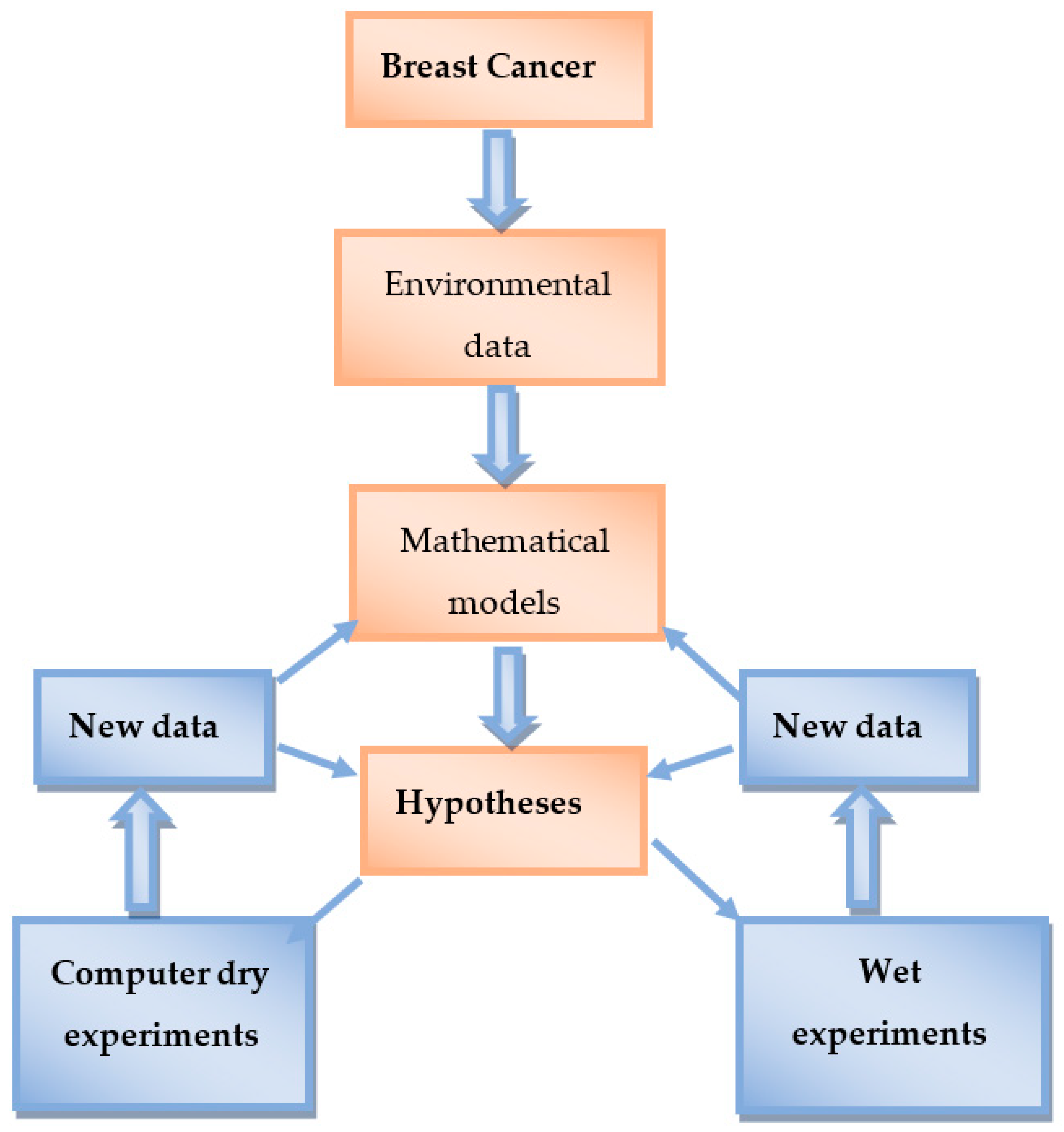
In this study, in a cooperative effort with our academic colleagues, in particular, clinicians and research oncologists, we devoted our attention to mathematical models of tumor growth with the objective of finding a better method of cancer treatment using mathematical concepts and ideas. This is illustrated in the Figure 1 flow diagram, where the various aspects of breast cancer are provided, which give useful information on its development, inversion and metastasis.

2. Mathematically Modeled Problems

From the various studies in the literature, it has been found both in vivo and in vitro that the growth of a tumor cell population is exponential for small quantities of tumor cells, but growth is slowed at large population sizes. The inhibition of growth may be caused by the competition of cells for metabolites or growth factors. In many instances of non-exponential tumor growth, the kinetics are well described by the logistic equation or Gompertz equation. For example, consider a nonlinear rigid system of ordinary differential equations [9] written as follows:
d y 1 ( t ) d t = σ + ρ y 1 ( t ) y 2 ( t ) η + y 2 ( t ) μ y 1 ( t ) y 2 ( t ) δ y 1 ( t ) , y 1 ( 0 ) = D , d y 2 ( t ) d t = α y 2 ( t ) ( 1 β y 2 ( t ) ) y 1 ( t ) y 2 ( t ) , y 2 ( 0 ) = D ,
where y 1 ( t ) are the effector cells, y 2 ( t ) are the tumor cells and [σ, ρ, η, μ, δ, α, β] are the parameters of the system, with values given as [0.1181, 1.131, 20.19, 0.00311, 0.3743, 1.636, 2.0 × 10⁻³], respectively. The practical solution of interest of the system in (1), that is, of the populations denoted by y 1 ( t ) , y 2 ( t ) can readily be obtained, which are assumed to be positive. We also assume that the parameters in the system are positive and the Ds are the initial conditions.
The second system of equations to be considered is another nonlinear stiff system [11], which are of the form:
d y 1 ( t ) d t = c y 2 ( t ) μ 2 y 1 ( t ) + p 1 y 1 ( t ) y 3 ( t ) g 1 + y 3 ( t ) + s 1 , y 1 ( 0 ) = D , d y 2 ( t ) d t = r 2 y 2 ( t ) ( 1 b y 2 ( t ) ) a y 1 ( t ) y 2 ( t ) g 2 + y 2 ( t ) , y 2 ( 0 ) = D , d y 3 ( t ) d t = p 2 y 1 ( t ) y 2 ( t ) g 3 + y 2 ( t ) μ 3 y 3 ( t ) + s 2 , y 3 ( 0 ) = D .
where all the parameter values are given in Table 1 and the Ds are also the initial conditions. The y 1 ( t ) is the effector-cells population, and s 1 is a treatment parameter, such as lymphokine-activated killed cell (LAK) therapy or tumor-infiltrating lymphocytes (TIL) therapy. The second equation is the tumor cells denoted by y 2 ( t ) and the third equation is the concentration of the interleukin-cells (IL-2) y 3 ( t ) . The s 2 is a treatment term which represents an external input of IL-2 into the system.
The third system of stiff equations recently considered by [7,14] to improve cancer treatment using chemotherapy and cancer stem cells is presented in (3). This has four systems of ODEs. The dynamic of the system is located in the nonnegative orthant:
R + , 0 4 = { y 1 0 ,   y 2 0 ,   y 3 0 ,   y 4 0 } . d y 1 ( t ) d t = γ 1 y 1 ( t ) k s y 1 ( t ) y 4 ( t ) , y 1 ( 0 ) = D , d y 2 ( t ) d t = α μ y 2 ( t ) + p 1 y 1 ( t ) y 2 ( t ) ( y 2 ( t ) + 1 ) p 2 ( y 3 ( t ) + y 4 ( t ) ) y 2 ( t ) , y 2 ( 0 ) = D , d y 3 ( t ) d t = r ( 1 b y 3 ( t ) ) y 3 ( t ) ( p 3 y 2 ( t ) + k T y 4 ( t ) ) y 3 ( t ) , y 3 ( 0 ) = D , d y 4 ( t ) d t = γ 2 y 4 ( t ) + v ( t ) , y 4 ( 0 ) = D
In the model, a competition amongst the cancer populations is formulated, which includes concentration of stem cells, effector cells, tumor cells and chemotherapy drug, respectively. We denote y 1 ( t ) as the stem cell concentration, y 2 ( t ) to represent the effector cells, y 3 ( t ) tumor cell concentration and lastly y 4 ( t ) as the chemotherapy drug concentration. All the constant parameters in the system are described in Table 2.
The last model was studied by [12,13], where y 1 ( t ) , y 2 ( t ) , y 3 ( t ) , y 4 ( t ) and y 5 ( t ) are, respectively, the cancer stem cells, tumor cells, healthy cells, immune cells and excess estrogen:
d y 1 ( t ) d t = k 1 y 1 ( t ) ( 1 y 1 ( t ) M 1 ) γ 1 y 1 ( t ) y 4 ( t ) + p 1 y 1 ( t ) y 5 ( t ) a 1 + y 1 ( t ) , y 1 ( 0 ) = D d y 2 ( t ) d t = k 2 y 1 ( t ) ( y 1 ( t ) M 1 ) ( 1 y 2 ( t ) M 2 ) n 1 y 2 ( t ) γ 2 y 2 ( t ) y 4 ( t ) + p 2 y 2 ( t ) y 5 ( t ) ( α 2 + y 2 ( t ) ) , y 2 ( 0 ) = D d y 3 ( t ) d t = q y 3 ( t ) ( 1 y 3 ( t ) M 3 ) δ y 2 ( t ) y 3 ( t ) p 3 y 3 ( t ) y 5 ( t ) a 3 + y 3 ( t ) . y 3 ( 0 ) = D d y 4 ( t ) d t = s + ρ y 2 ( t ) y 4 ( t ) ω + y 2 ( t ) γ 3 y 2 ( t ) y 4 ( t ) n 2 y 4 ( t ) u y 4 ( t ) y 5 ( t ) v + y 5 ( t ) , y 4 ( 0 ) = D d y 5 ( t ) d t = r ( μ + d 1 y 1 ( t ) a 1 + y 1 ( t ) + d 2 y 2 ( t ) a 2 + y 2 ( t ) + d 3 y 3 ( t ) a 3 + y 3 ( t ) ) y 5 ( t ) , y 5 ( 0 ) = D
where some of the parameters in the system are described in Table 3, while others are described as follows: { ρ } represents the immune cell response and { a 1 , a 2 , a 3 } represent the number of y 1 ( t ) , y 2 ( t ) , y 3 ( t ) cells. The values { p 1 , p 2 , p 3 } help estrogen to proliferate cancer stem cells, tumor cells and the rate at which healthy cells are lost to DNA mutation due to the presence of estrogen. The absorption of estrogen by cancer stem cells, tumor cells and healthy cells are denoted by the values { d 1 , d 2 , d 3 } , respectively.
Our major worry about all the mathematical models developed and studied is the determination of the solutions. Almost all the methods used for the solution of the models, except in the first model (1) which is experimental or practical in nature, are of lower orders and tend to have undesirable time-step restrictions and poor stability properties within the domain of solution. It is of interest to have method(s) with high accuracy and the ability to incorporate some function evaluations at some off-grid points which are widely used in continuous applications to solve real-life problems.

3. Numerical Computational Algorithms

Ordinary differential equations play an important role in the physical sciences, engineering, biological sciences, technology, etc. Some of these equations have difficulty (stiff) in obtaining their solutions, even numerically. These type of differential equations have arisen in several areas of interest, such as medicine, anthropology, engineering and many other fields. However, only very few of these differential equations can be solved analytically. In this paper, we develop continuous block implicit hybrid methods (CBHMs) based on Chebyshev polynomial nodes that have better regions of absolute stability (RAS) over a wide parameter range. The numerical computation of the study is called continuous block implicit hybrid methods (CBHMs) obtained from the Chebyshev points, with the general form as follows:
y ( x ) = j = 0 r ν j ( x ) y n + j + j = 0 s υ j ( x ) f ( x ¯ n + j , y ( x ¯ n + j ) ) , j = 0 , 1 , 2 , , s .
where
y n + j = y ( x n + j h ) ,
y n + j = f n + j = f ( x ¯ n + j h , y ( x ¯ n + j h ) )
We denote the number of interpolation points x n + j ,   j = 0 , 1 , 2 , , r 1 , by r taken from ( x n , x n + 1 ) , and denote the distinct collocation points x ¯ n + j ,   j = 0 , 1 , 2 , , s 1 by s, also chosen from the interval [ x n , x n + 1 ] . The continuous coefficients ν j ( x ) and υ j ( x ) in (5) are to be determined. They are of degree p 1 ( p = r + s ) given by:
ν j ( x ) = i = 0 p 1 ν j , i + 1 x i   and   h υ j ( x ) = h i = 0 p 1 υ j , i + 1 x i .
The coefficients ν j , i + 1 and υ j , i + 1 in (7) are to be determined explicitly.
Theorem 3.1.
Collocation at the Gaussian points together with the two end points lead to order one less than the superconvergence scheme, while collocation at only one additional end point to the Gaussian points resulted in order two less than the upgraded scheme.
Proof .
(see [17,18,19]). □
Case I:
We shall derive one-step collocation methods as continuous block implicit hybrid formulae of orders 3 and 4. We shall consider the zeros of the Chebychev polynomial of degree 3, which can be normalized to give the general finite range in a x b as:
T n * ( x ) = cos ( n arccos ( t ) ) , t = 2 x ( b + a ) b a
Hence, with n = 3, we obtain the zeros of the Chebyshev polynomial as follows:
x ¯ 0 = x n + u , u = ( 2 3 ) / 4 x ¯ 1 = x n + w , w = 1 2 x ¯ 2 = x n + v , v = ( 2 + 3 ) / 4 }
In this family r = 1 , s = 3 , ξ = ( x x n ) , the continuous scheme is given as:
y ( x ) = ν 0 ( x ) y n + h [ υ 1 ( x ) f n + u + υ 2 ( x ) f n + w + υ 3 ( x ) f n + v ] .
where
ν 0 ( x ) = 1 υ 1 ( x ) = [ 2 ( x x n ) 3 3 ( v + w ) h ( x x n ) 2 + 6 v w h 2 ( x x n ) 6 ( v u ) ( w u ) h 2 ] , υ 2 ( x ) = [ 2 ( x x n ) 3 3 ( v + u ) h ( x x n ) 2 + 6 v u h 2 ( x x n ) 6 ( w u ) ( w v ) h 2 ] , υ 3 ( x ) = [ 2 ( x x n ) 3 + 3 ( u + w ) h ( x x n ) 2 + 6 u w h 2 ( x x n ) 6 ( v u ) ( w v ) h 2 ]
Evaluating (8), we obtain the continuous block implicit hybrid method of order 4 with only 3 stages written in the form:
y n + 1 = y n + h 9 [ 2 f n + u + 5 f n + w + 2 f n + v ] ,   order   p = 4 ,   C 5 = 1.3020 × 10 4
y n + u = y n + h 144 [ ( 16 3 3 ) f n + u + ( 40 24 3 ) f n + w + ( 16 9 3 ) f n + v ] , order   p = 3 ,   C 4 = 1.6276 × 10 4
y n + w = y n + h 36 [ ( 4 + 3 3 ) f n + u + 10 f n + w + ( 4 3 3 ) f n + v ] , order   p = 3 ,   C 4 = 1.3020 × 10 4
y n + v = y n + h 144 [ ( 16 + 9 3 ) f n + u + ( 40 + 24 3 ) f n + w + ( 16 + 3 3 ) f n + v ] , order   p = 3 ,   C 4 = 1.3020 × 10 4
Note that the matrix 
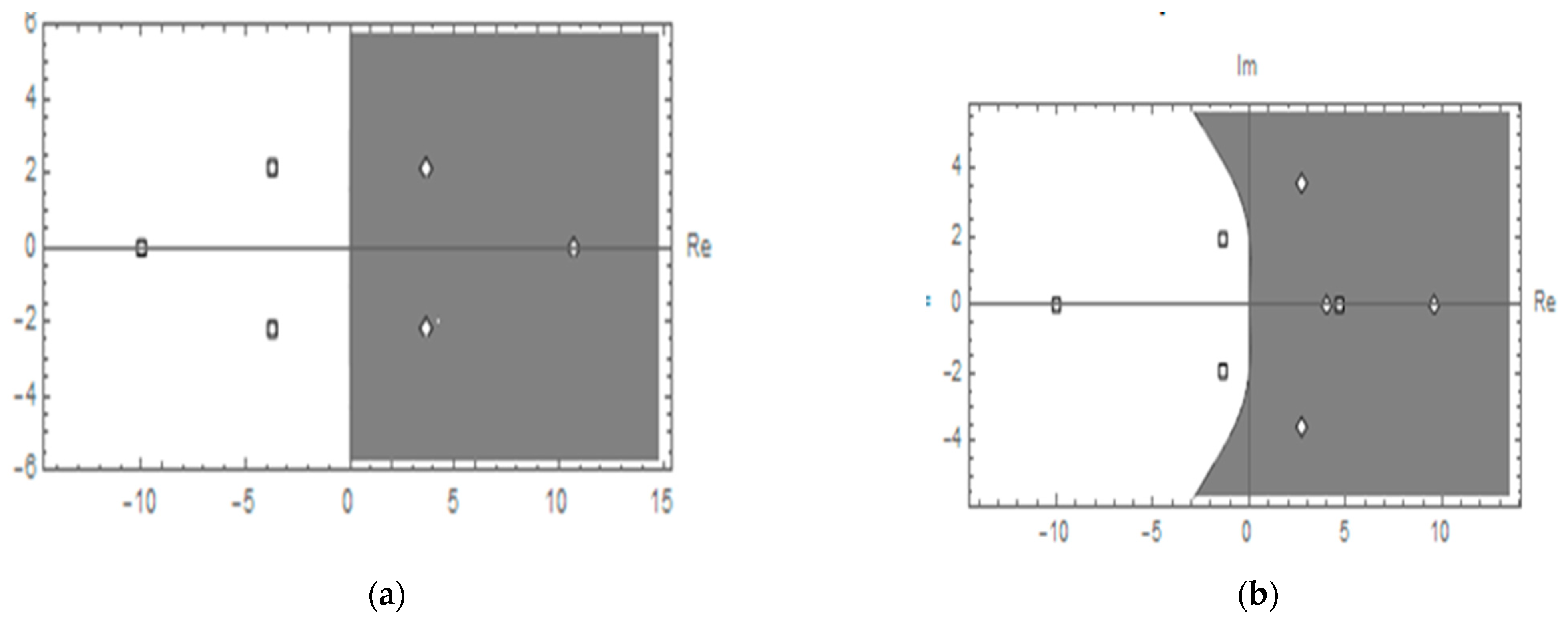
A obtained from the derived method is not a lower triangular matrix hence it is a fully dense matrix, that is, a fully implicit method. In addition, it has higher order than the explicit case, which has fewer stages too. Using the maple package, yields the stability polynomial of the block implicit hybrid method as
p ( η , z ) = η ( z 3 + η z 3 + 18 z 2 18 η z 2 + 96 η z 192 η + 96 z + 192 ) z 3 18 z 2 + 96 z 192
The RAS of the block implicit hybrid method is plotted using the MATLAB package as shown in Figure 2a.
Case II:
Collocating at the three interior points above and one additional end point we obtain the continuous scheme:
y ( x ) = ν 0 ( x ) y n + h [ υ 1 ( x ) f n + u + υ 2 ( x ) f n + w + υ 3 ( x ) f n + v + υ 4 ( x ) f n + 1 ]
where
ν 0 ( x ) = 1 ,
υ 1 ( x ) = [ ( x x n ) 4 + 4 ( v + u + w ) h ( x x n ) 3 6 ( v u + v w + u w ) h 2 ( x x n ) 2 + 12 v u w h 3 ( x x n ) 12 ( v 1 ) ( u 1 ) ( w 1 ) h 3 ] ,
υ 2 ( x ) = [ 3 ( x x n ) 4 4 ( v + w + 1 ) h ( x x n ) 3 + 6 ( v w + v + w ) h 2 ( x x n ) 2 12 v w h 3 ( x x n ) 12 ( v u ) ( w u ) ( u 1 ) h 3 ] ,
υ 3 ( x ) = [ 3 ( x x n ) 4 + 4 ( v + u + 1 ) h ( x x n ) 3 6 ( v u + v + u ) h 2 ( x x n ) 2 + 12 v u h 3 ( x x n ) 12 ( v w ) ( w u ) ( w 1 ) h 3 ] ,
υ 4 ( x ) = [ 3 ( x x n ) 4 4 ( u + w + 1 ) h ( x x n ) 3 + 6 ( u w + u + w ) h 2 ( x x n ) 2 12 u w h 3 ( x x n ) 12 ( v u ) ( v w ) ( v 1 ) h 3 ] .
Evaluating (10) at the off-step points x n + u , x n + w , x n + v and at the end point x n + 1 , the following continuous block implicit hybrid method is obtained as follows:
y n + 1 = y n + h 9 [ 2 f n + u + 5 f n + w + 2 f n + v ] , order   p = 4 ,   C 5 = 1.3020 × 10 4
y n + u = y n + h 288 [ ( 38 9 3 ) f n + u + ( 77 48 3 ) f n + w + ( 38 15 3 ) f n + v 9 f n + 1 ]   order   p = 4 ,   C 5 = 3.9813 × 10 5
y n + w = y n + h 36 [ ( 2 6 3 ) f n + u + 13 f n + w ( 2 + 6 3 ) f n + v + 9 f n + 1 ]   order   p = 4 ,   C 5 = 2.2786 × 10 4
y n + v = y n + h 288 [ ( 38 + 15 3 ) f n + u + ( 77 + 48 3 ) f n + w + ( 38 + 9 3 ) f n + v 9 f n + 1 ]   order   p = 4 ,   C 5 = 3.9813 × 10 5
The continuous block implicit hybrid method of uniform order p = 4 everywhere in the interval of the solution is obtained for the solution of dynamics breast cancer models. Using the MAPLE package yields the stability polynomial of the method as:
p ( η , z ) = η ( 768 η + 132 η z 2 19 η z 3 + η z 4 480 η z 768 36 z 2 z 4 288 z ) z 4 19 z 3 + 132 z 2 480 z + 768
The RAS of the continuous block implicit hybrid method was plotted using MATLAB package as shown in Figure 2b.
Regions of absolute stability of the continuous block implicit hybrid methods which are A-stable and symmetric about the x-axis, since the enclosed Figures of the regions contain the complex plane outside the domain.
From the two block implicit hybrid methods obtained, it is clear that the Chebyshev polynomial roots are a good approximant of ordinary differential equations. Evidently, Ibiejugba and Onumanyi [20] pointed out that the selection of the elements using the zeros of some appropriate Chebyshev polynomials yield some interesting properties, such as the satisfaction of the usual local support. According to the authors, the idea of selecting the elements based on the zeros of Chebyshev polynomials as described in their paper is in line with the principle of the “orthogonal collocation method” or “method of selected points”.

4. Results and Discussion

Many mathematical models of interactions between the immune system, chemotherapies (anticancer agents) and the growing tumor have been developed in the recent literature. Immunotherapies which are responsible for stimulating antigen-sensitized cells are becoming a very significant component for treating cancer. This can easily be done by increasing the number of effector cells, either by stem cell transformation or by using the combination of cytokine interleukin-2 together with adoptive cellular immunotherapy, which will have the energy to fight the tumor cells by reducing their number and strength. This has been demonstrated in the laboratory and also in clinical experiments (see, for example, Farrar et al. [21], O’Byrne et al. [22], and de Pillis et al. [23]). Apparently, immune system cells usually attacked and killed cancer cells and therefore kept cancer incidence very low (see [24,25]).
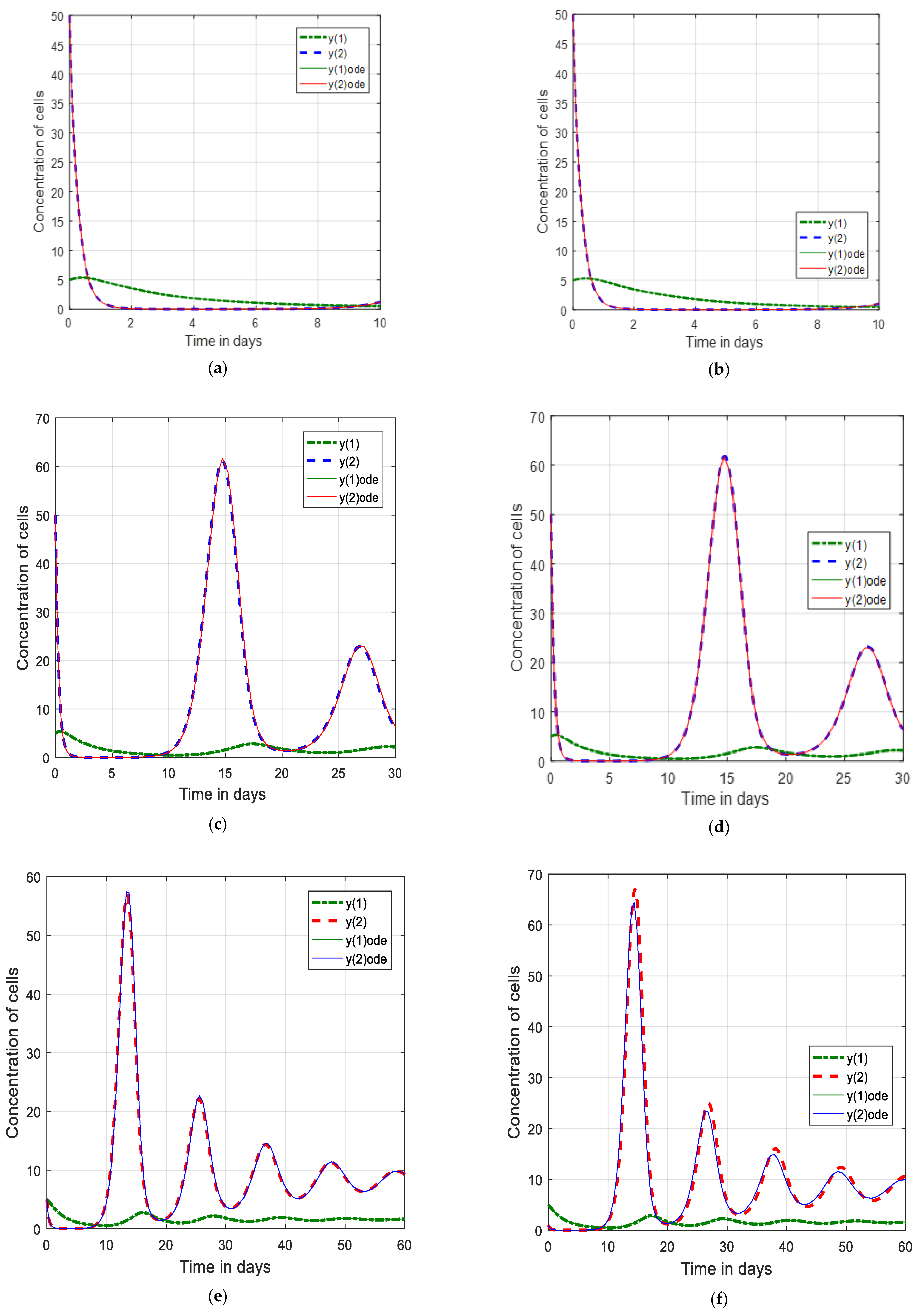
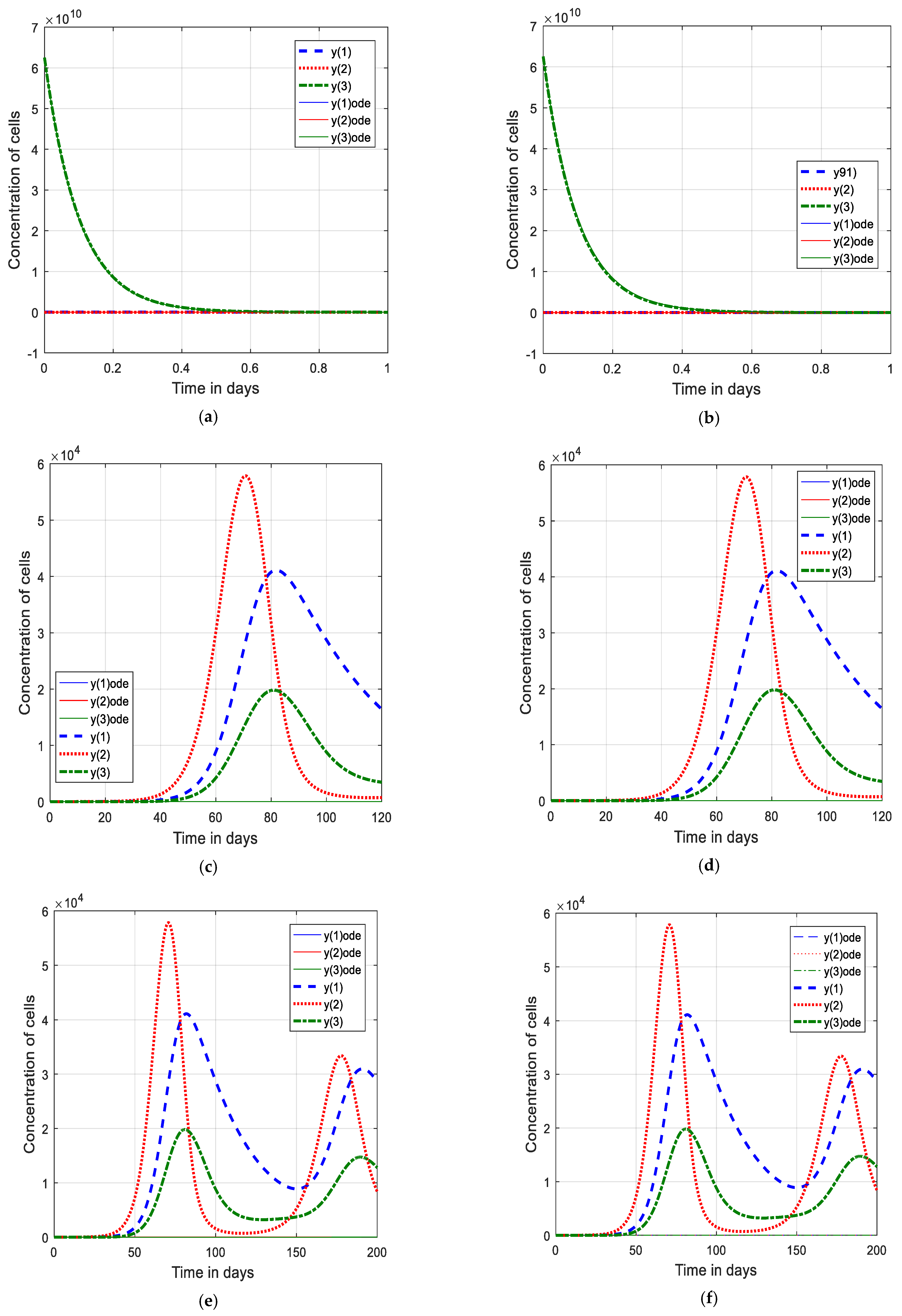
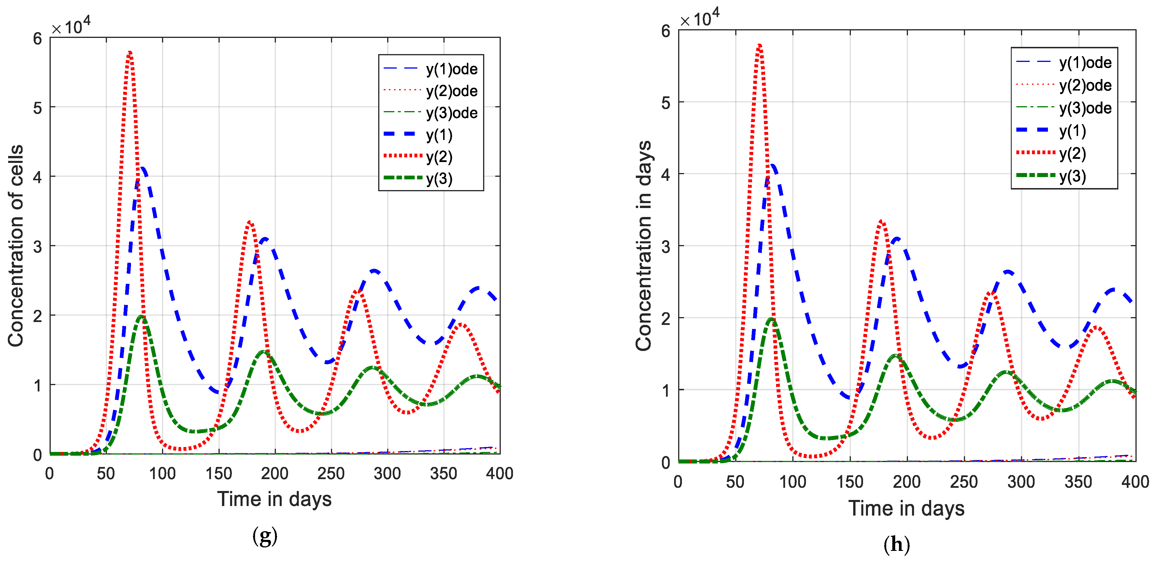
From the Figures showing the graphical representation of the results in this section, transients near the steady state show decaying oscillations in the plots. The graphical representations of the results, for example, Figure 3 and Figure 4, are of interest due to the fact that they portrait stable limit cycles, showing that the tumor and the immune system are subject to oscillations. In some cases, cyclic fluctuations in the number of leukocytes were observed. We noticed from the given graphical representation of the results that the system can be stable only if the given immune resistance is greater than the tumor growth. The graphs of Figure 3 for y 1 ( 0 ) = 5 and y 2 ( 0 ) = 50 in the neighborhood are clearly depicted (presented). The plots of Figure 3c–f for one and two months are in good agreement with certain human leukemia found in the literature (see, for example, [9,11,23]). In the graphs of Figure 3g–j, decaying oscillations to a dormant tumor state are also clearly depicted. However, in the case of higher doses for a longer period of time, the system evolves to an oscillatory state, as shown or depicted in Figure 3g–j. However, in the graphs of Figure 3a,b, as we can see, the effect is small because of the number of days considered. From Figure 3a,b, no oscillation is experienced in the graphs.
The parameter estimates in Table 1 are biologically reasonable because they characterize tumor growth in the absence of an immune response and the data determine the slope and asymptotes of the tumor growth curves. From the efficiency curves generated using Equation (2) or Model II, we can make a number of biological predictions about the interactions of the immune system with the growth tumor, as we did in Equation (1) or Model I. Compared with some published results in scientific articles, cyclic fluctuations in the number of leukocytes were found in several cases (see, for example [8,10]).
Practically, Equation (2) described the interaction amongst the effector cells y 1 ( t ) , tumor cells y 2 ( t ) and the cytokine interleukin-2(IL-2) y 3 ( t ) . As shown in the graphical plots of Figure 4, the initial points, even before introducing the treatment, were almost the same: these are y 1 ( 0 ) = 1 × 10 7 , y 2 ( 0 ) = 3 × 10 5 , y 3 ( 0 ) = 0.25 × 10 10 or y 1 ( 0 ) = y 2 ( 0 ) = y 3 ( 0 ) = 1 or y 1 ( 0 ) = y 2 ( 0 ) = y 3 ( 0 ) = 0. The idea, then, is to improve the natural immune system by using (IL-2), which is usually used together with adoptive cellular immunotherapy (ACI). Cytokines, which are stimulating protein hormones, enhance both natural and specific immunity (effector cells). Here, we indicate the treatment s 1 in the equation as the use of adoptive cellular immunity (ACI). Administering a large amount of the interleukin-2(IL-2), which is denoted by s 2 in the equation, yields an interesting result. It completely cleared the tumor cells but also has the side effect of capillary leakage syndrome (or vascular leakage syndrome) according to some eminent authors (see, for example, [26,27]). As observed in 
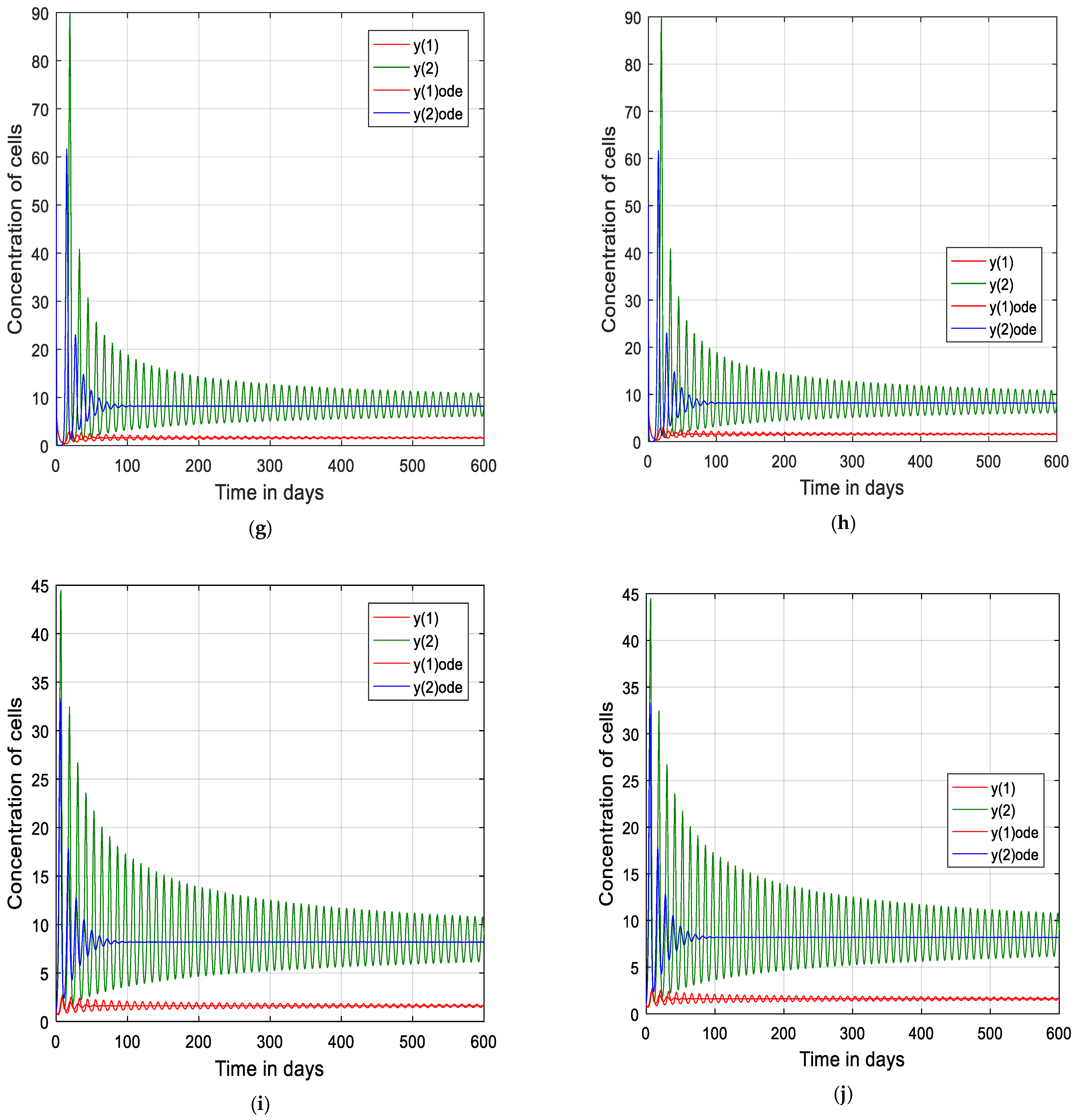
Figure 3i,j, which are very similar, the difference in oscillations is connected or linked with the values of the initial dose.
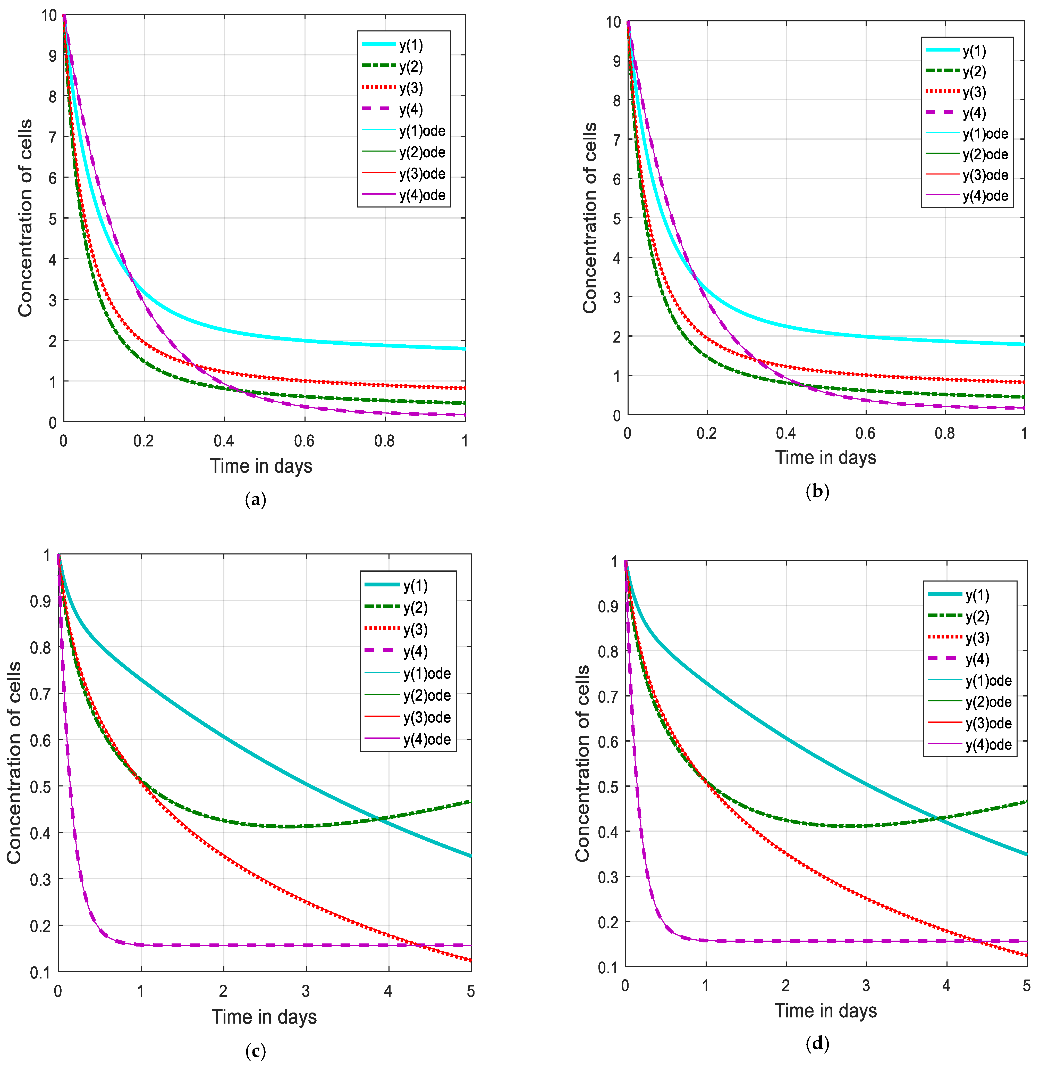
As shown in the graphs of Figure 5, the tumor cell population reduced by using only a small constant initial dose of chemotherapy for a short period of time. The idea of using the continuous block implicit hybrid methods is to accurately determine solutions of the modeled differential equations so that even a minimum initial dose of treatment, that is, the last term of Equation (3), V M , will be able to reduce (Figure 5a,b,g,h) or eliminate (Figure 5c,d,e,f) the tumor population described by Equation (3), that is, the term V ( t ) in the equation. In the recent literature, some authors, for example, de Pillis et al. [28], suggested the use of a high dose for a few days to eliminate the tumor. Though, if one uses high dose for few days, we observed that the case of increase in immune cells will cause a serious side effect of the treatment, as discussed in the case of the graphs of Figure 4 above. As can be seen in Figure 5, our solution graphs differ from that of Figure 4 in terms of the initial dose and the period of applications, which guaranteed complete tumor clearance without much side effect.
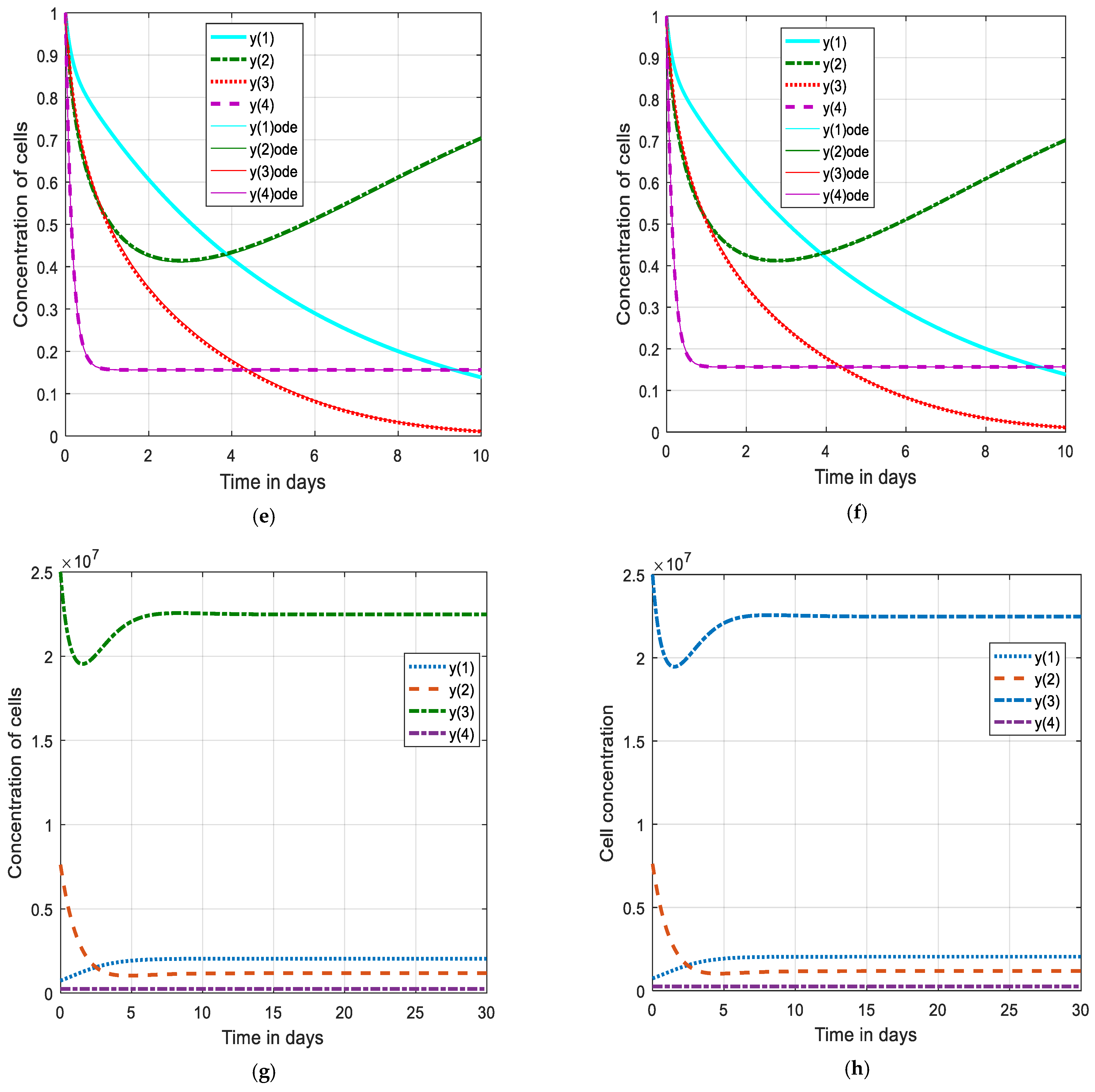
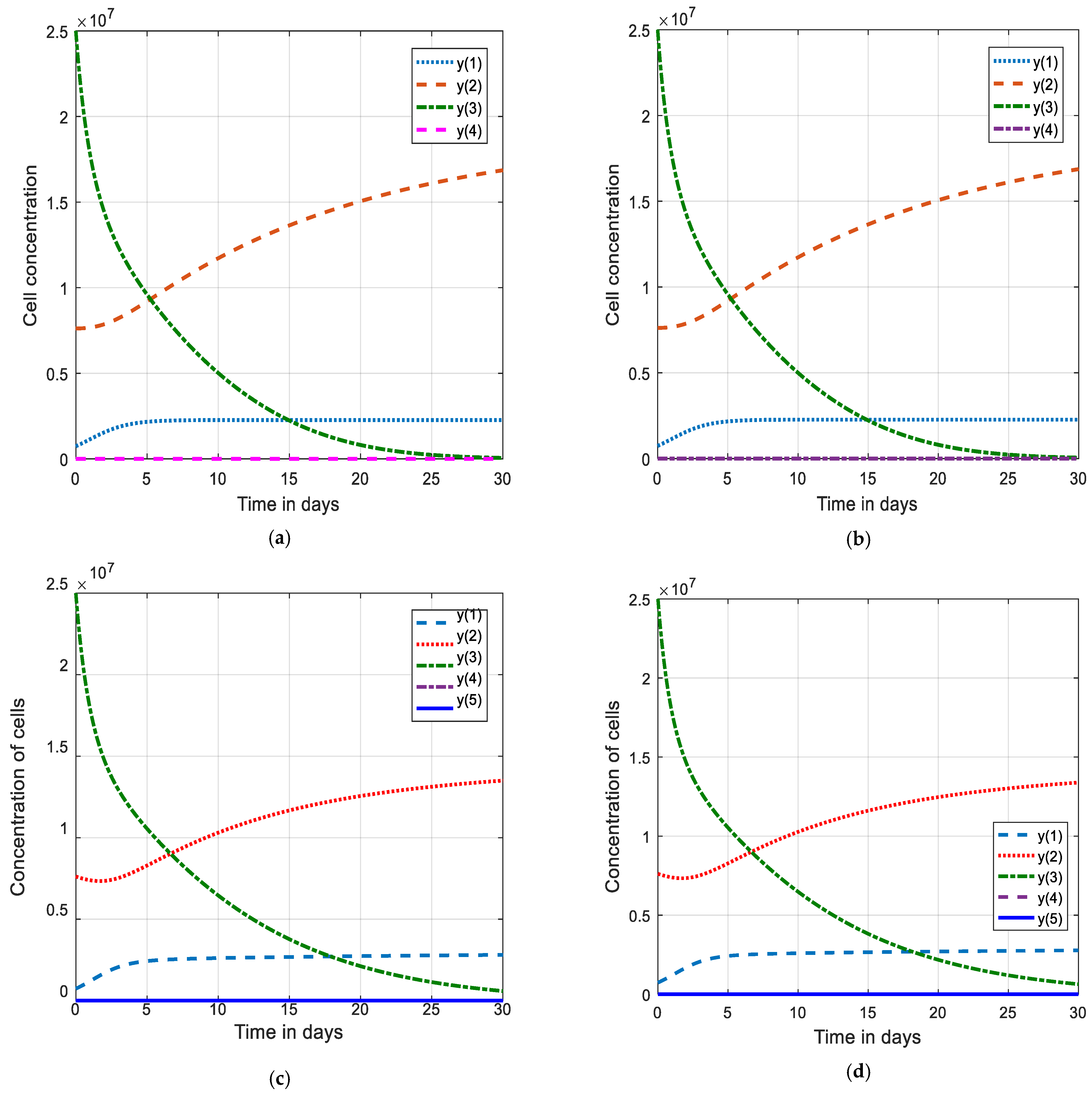
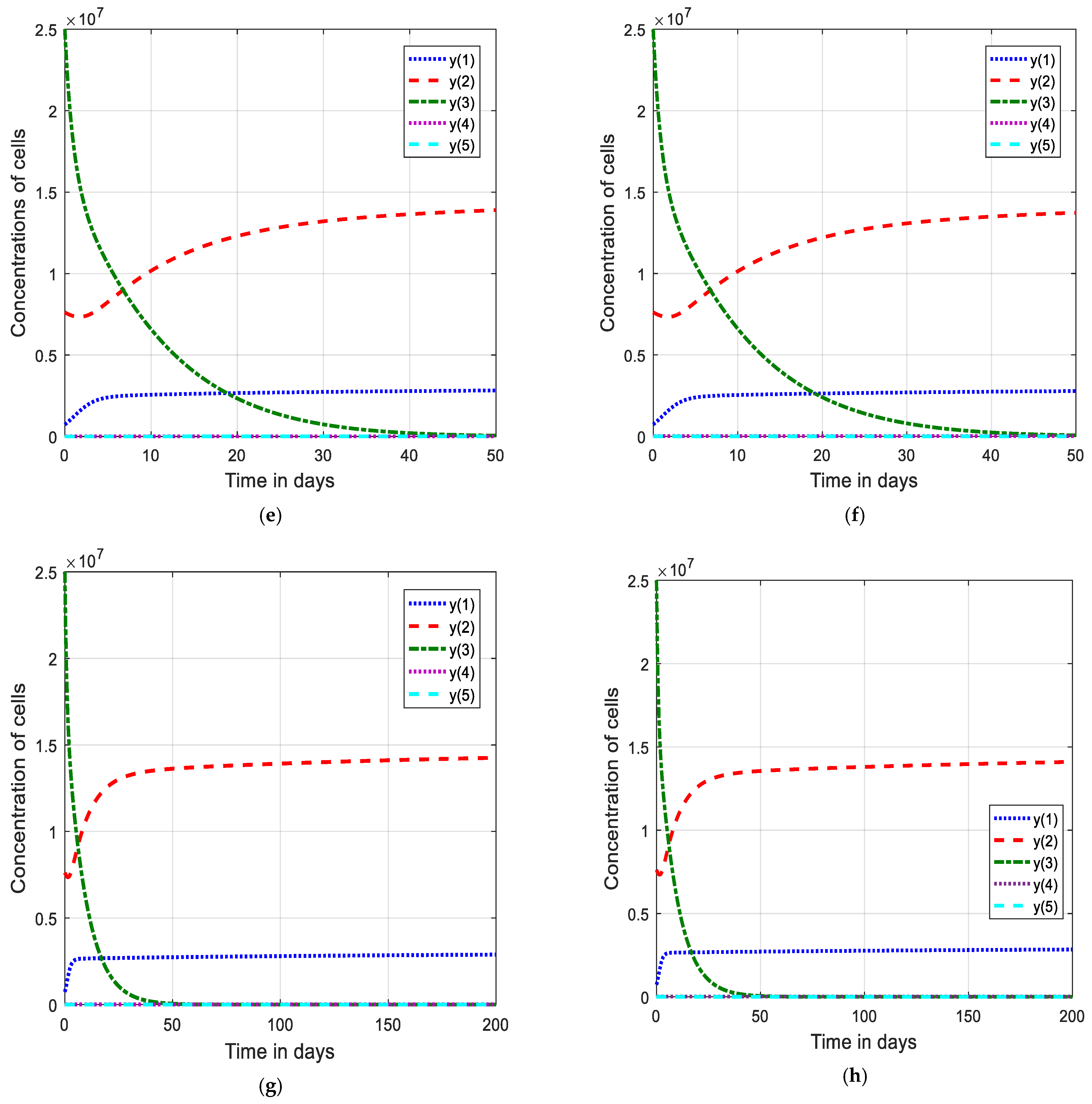
In Figure 6, we solved and analyzed a model of cancer disease which considered five populations involving y 1 ( t ) , y 2 ( t ) , y 3 ( t ) , y 4 ( t ) and y 5 ( t ) , which are cancer stem cells, tumor cells, healthy cells, immune cells and excess estrogen, respectively [6,13]. As seen in Figure 6a,b, which depicts the behavior of the graphs of the sub-model without estrogen over time, with cancer stem cells, tumor cells, healthy cells and immune cells all beginning at their carrying capacities, cancer still persists at a very high level. If observed carefully, the natural immune cell is not sufficient to even reduce the cancer, much less completely eradicate the tumor, as observed in [6,13,29].
Further, from the graphs of the Figure, it is clearly shown that the presence of excess estrogen, tumor cells increase, but immune cells and healthy cells decrease. In such a situation the normal cells are very much being affected, which makes the system unstable. As can be seen in Figure 6c–h, with the increase in estrogen levels, the immune levels are completely reduced, thereby weakening the body’s immune system [13]. This suggests that, in the presence of excess estrogen, all breast tissue eventually becomes infected with tumor cells. Here, we advise that taking extra levels of estrogen, either as hormonal birth control or to enhance beauty, ends up practically increasing the risk of developing breast cancer and should therefore be avoided.

5. Conclusions

Biological systems are very close to clinical medicine. This is because experiments are performed to test samples. This is where mathematical models are significant, especially in biomedical science where some complex biological models are tested. In this study, we have illustrated how mathematical techniques could be used in biology and medicine, which are difficult to achieve through experimental work alone. These results could prove important and useful in our efforts to effectively deliver a variety of novel and exciting immunotherapies, particularly the cytokine interleukin-2, adoptive cellular immunotherapy, etc. Overall, the study shows that early treatment is the best way to eliminate the tumor. Hence, our results presented should be useful, especially for choosing the optimal treatment strategy which does not cause great negative impact on the cancer patient as demonstrated above graphically. It is interesting to note that in this article we provide a graphical representation of the results obtained from the solutions of modeled equations where the singular control is optimal with respect to the solutions. Therefore, the simulated results presented here show that the CBHMs are good candidates for generating results that represent various asymptomatic behaviors that track the real data more closely than most of the methods used in the literature. We hope that the methods used here can be applied to other biologically complex models.

Author Contributions

Writing—original draft preparation, D.G.Y. and K.S.A.; funding acquisition, M.Y.A.; methodology and supervision, A.M. and A.G.T. All authors contributed equally to this work. All authors have read and agreed to the published version of the manuscript.

Funding

This research was funded by Tertiary Education Trust Fund (TETFund).

Data Availability Statement

Not applicable (no data were used during the study).

Acknowledgments

The authors gratefully acknowledge the financial support of the TETFUND. The authors are also grateful to the anonymous reviewers and the handling editor for their constructive comments, observations and suggestions which enhanced the paper.

Conflicts of Interest

The authors declare no conflict of interest for the study.

References

  1. Brahimi-Horn, M.C.; Chiche, J.; Pouyssegur, J. Hypoxia and cancer. J. Mol. Med. 2007, 85, 1301–1307. [Google Scholar] [CrossRef] [PubMed] [Green Version]
  2. Furlani, E.P.; Ng, K.C. Analytical model of magnetic nanoparticles transport and capture in the microvasculature. Phys. Rev. E 2006, 73, 061919. [Google Scholar] [CrossRef] [PubMed] [Green Version]
  3. Furlani, E.J.; Furlani, E.P. A model for predicting magnetic targeting of multifunctional particles in the microvasculature. J. Magt. Magt. Mater. 2007, 312, 187–193. [Google Scholar] [CrossRef] [Green Version]
  4. Liyanage, P.Y.; Hettiarachchi, S.D.; Zhou, Y.; Ouhtit, A.; Seven, E.S.; Oztan, C.Y.; Celik, E.; Leblanc, R.M. Nanoparticles-mediated targeted drug delivery for breast cancer treatment. BBA Rev. Cancer 2019, 1871, 419–433. [Google Scholar] [CrossRef] [PubMed]
  5. Atangana, A.; Jain, S. The role of power decay, exponential decay and Mittag-Leffler function’s waiting time distribution: Application of cancer spread. Physica A 2018, 512, 330–351. [Google Scholar] [CrossRef]
  6. Mufudza, C.; Sorofa, W.; Chiyaka, E.T. Assessing effects of estrogen on the dynamics of breast cancer. Comput. Math. Meth. Med. 2012, 2012, 473572. [Google Scholar] [CrossRef] [Green Version]
  7. Valle, P.A.; Starkova, K.E.; Coria, L.N. Global stability and tumor clearance conditions for a cancer chemotherapy system. Commun. Nonl. Scie. Numer. Simul. 2016, 40, 206–215. [Google Scholar] [CrossRef]
  8. de Lisi, C.; Rescigno, A. Immune surveillance and neoplasia-1: A minimal mathematical model. Bull. Math. Biol. 1977, 39, 201–221. [Google Scholar]
  9. Kuznetsov, V.A.; Makalkin, I.A.; Taylor, M.A.; Perelson, A.S. Nonlinear dynamics of immunogenic tumors: Parameter estimation and global bifurcation analysis. Bull. Math. Biol. 1994, 56, 295–321. [Google Scholar] [CrossRef]
  10. Adams, J.A. Effects of vascularization on lymphocyte/tumor cell dynamics: Qualitative features. Math. Comput. Model. 1996, 23, 1–10. [Google Scholar] [CrossRef] [Green Version]
  11. Kirschner, D.; Panetta, J.C. Modeling immunotherapy of the tumor-immune interaction. J. Math. Bio. 1998, 37, 235–252. [Google Scholar] [CrossRef] [Green Version]
  12. Abernathy, K.; Abernathy, Z.; Baxter, A.; Stevens, M. Global dynamics of a breast cancer competition model. Diff. Equ. Dyn. Syst. 2020, 28, 791–805. [Google Scholar] [CrossRef]
  13. Solis-Perez, J.E.; Gomez-Aguilar, J.F.; Atangana, A. A fractional mathematical model of breast cancer competition model. Chaos Solitons Fractals 2019, 127, 38–54. [Google Scholar] [CrossRef]
  14. Alqudah, M.A. Cancer treatment by stem cells and chemotherapy as a mathematical model with numerical simulations. Alex Eng. J. 2020, 59, 1953–1957. [Google Scholar] [CrossRef]
  15. Simmons, A.; Burrage, P.M.; Nicolau, D.V., Jr.; Lakhani, S.R.; Burrage, K. Environmental factors in breast cancer invasion: A mathematical modelling review. J. Pathol. 2017, 49, 172–180. [Google Scholar] [CrossRef] [Green Version]
  16. Oke, S.I.; Matadi, M.B.; Xulu, S.S. Optimal control analysis of mathematical model for breast cancer. J. Math. Comput. Appl. 2018, 23, 21. [Google Scholar]
  17. Yakubu, D.G.; Markus, S.; Amina, H.; Kwami, A.M. Symmetric uniformly accurate Gauss Runge-Kutta method. Leonardo J. Sci. 2007, 11, 113–122. [Google Scholar]
  18. Kwami, A.M.; Kumleng, G.M.; Kolo, A.M.; Yakubu, D.G. Block hybrid multistep methods for the numerical integration of stiff systems of ordinary differential equations arising from chemical reactions. Abacus. J. Math. Ass. Nig. 2016, 42, 134–164. [Google Scholar]
  19. Yakubu, D.G.; Manjak, N.H.; Buba, S.S.; Maksha, A.I. A family of uniformly accurate order Runge-Kutta collocation methods. J. Comput. Appl. Math. 2011, 30, 315–330. [Google Scholar] [CrossRef] [Green Version]
  20. Ibiejugba, M.A.; Onumanyi, P. On some new Chebyshev polynomial basis functions in C0 space. In Proceedings of the First International Conference on Numerical Analysis and Its Applications, Benin City, Nigeria, 2–4 November 1983; pp. 120–126. [Google Scholar]
  21. Farrar, J.D.; Katz, K.H.; Windsor, J.; Thrush, G.; Scheuermann, R.H.; Uhr, J.W.; Street, N.E. Cancer dormancy. VII. A regulatory role for CD8+ T cells and IFN-gamma in establishing and maintaining the tumor-dormant state. J. Immune 1999, 162, 2842–2849. [Google Scholar]
  22. O’Byrne, K.J.; Dalgleish, A.G.; Browning, M.J.; Steward, W.P.; Harris, A.L. The relationship between angiogenesis and the immune response in carcinogenesis and the progression of malignant disease. Eur. J. Cancer 2000, 36, 151–169. [Google Scholar] [CrossRef]
  23. de Pillis, L.G.; Gu, W.; Radunskaya, A.E. Mixed immunotherapy and chemotherapy of tumors: Modeling applications and biological interpretations. J. Theor. Biol. 2006, 238, 841–862. [Google Scholar] [CrossRef] [PubMed]
  24. Baleanu, D.; Jajarmi, A.; Sajjadi, S.S.; Mozyrska, D. A new fractional model and optimal control of a tumor-immune surveillance with nonsingular derivative operator. J. Chaos Interdiscip. J. Nonlinear Sci. 2019, 29, 083127. [Google Scholar] [CrossRef]
  25. Mahasa, K.J.; Ouifki, R.; Eladdadi, A.; de Pillis, L. Mathematical model of tumor-immune surveillance. J. Theor. Biol. 2016, 404, 10312–10330. [Google Scholar] [CrossRef] [PubMed] [Green Version]
  26. Lee, R.E.; Lotze, M.T.; Skibber, J.M.; Tucker, E.; Bonow, R.O.; Ognibene, F.P.; Carrasquillo, J.A.; Shelhamer, J.H.; Parillo, J.E.; Rosenberg, S.A. Cardiorespiratory effects of immunotherapy with interleukin-2. J. Clin. Onco. 1989, 7, 7–20. [Google Scholar] [CrossRef]
  27. Lissoni, P.; Barni, S.; Cattaneo, G.; Archili, C.; Crispino, S.; Tancine, G.; D’Angelo, L.; Magni, S.; Fiorelli, G. Activation of the complement system during immunoltherapy of cancer with interleukin-2: A possible explanation of the capillary leak syndrome. Inter. J. Biol. Markers 1990, 5, 195–197. [Google Scholar] [CrossRef]
  28. de Pillis, L.G.; Gu, W.; Fister, K.R.; Head, T.; Maples, K.; Murugan, A.; Neal, T.; Yoshida, K. Chemotherapy for tumors: An analysis of the dynamics and a study of quadratic and linear optimal controls. J. Math. Biosci. 2007, 209, 292–315. [Google Scholar] [CrossRef] [PubMed]
  29. Abubakar, M.; Abdulhameed, M.; Kwami, A.M.; Abdullahi, A.; Markus, S.; Yakubu, D.G. Numerical simulation of mathematical model for cancer treatments by stem cells and chemotherapy using Caputo-Fabrizio fractional derivative. Int. J. Inno. Sci. Res. Rev. 2022, 3, 2494–2504. [Google Scholar]
Figure 1. Mathematical models to generate and refine hypotheses of breast cancer.
Fractalfract 07 00237 g001
Figure 2. Stability regions of method (9) (a) and method (11) (b) with poles inclusive.
Fractalfract 07 00237 g002
Figure 3. Illustration of decay oscillation to the dormant tumor state of the rate of concentration of the effector cells and IL-2 along the time t in days, y 1 ( t ) [ ] effector cells, and y 2 ( t ) [ ] tumor cells.
Fractalfract 07 00237 g003aFractalfract 07 00237 g003b
Figure 4. Rate of concentration of cells along the time t in days, y 1 ( t ) [ ] effector cells, y 2 ( t ) [ ] tumor cells and y 3 ( t ) [ ] immune response.
Fractalfract 07 00237 g004aFractalfract 07 00237 g004b
Figure 5. Rate of concentration of cells and drug along the time t in days, y 1 ( t ) [ ] stem cells, y 2 ( t ) [ ] effector cells, y 3 ( t ) [ ] tumor cells, y 4 ( t ) [   ] drug concentration.
Fractalfract 07 00237 g005aFractalfract 07 00237 g005b
Figure 6. Rate of concentration of cells along the time t in days, stem cells y 1 ( t ) [ ] , tumor cells y 2 ( t ) [   ] , healthy cells y 3 ( t ) [ ] , immune cells y 4 ( t ) [ ] , estrogen y 5 ( t ) [   ] .
Fractalfract 07 00237 g006aFractalfract 07 00237 g006b
Table 1. Parameter values.
0 c 0.05 μ 2 = 0.03 p 1 = 0.1245 g 1 = 2 × 10 7
g 2 = 1 × 10 5 r 2 = 0.18 b = 1 × 10 9 a = 1
g 2 = 1 × 10 5 p 2 = 5 g 3 = 1 × 10 3
Table 2. Parameter values in different models of drug concentration.
ParameterInterpretationValue
y 1 ( 0 ) Initial concentration of stem cells1
y 2 ( 0 ) Initial concentration of effector cells1
y 3 ( 0 ) Density of free tumor1
γ 1 Decay rate of stem cells concentration−0.02825
α Rate of product of the effector cells0.17
μ Natural death rate of the effector cells0.03
b Carrying capacity of the tumor cells10−9
k s Fractional stem cells killed by chemotherapy1
p 1 Maximum proliferation rate of effector cells0.1245
r Tumor growth rate0.18
p 2 Decay rate of the effector cells killed by
tumor cells and chemotherapy
1
k T Fractional tumor cells killed by chemotherapy0.9
p 3 Decay rate of tumor cells killed by the effector cells0.9
γ 2 Decay rate of chemotherapy drug 6.4
y 4 ( 0 ) The time dependent external influx of
chemotherapy drug
1
Table 3. Parameter values in different models of drug concentration.
ParameterInterpretationValue
k 1 Rate of y 1 cells division0.75 day−1
k 2 Rate of y 2 cells division0.514 day−1
q Rate of y 3 cells division 0.70 day−1
M 1 Carrying capacity of y 1 cells 2.27 × 10 6 cells y 1
M 2 Carrying capacity of y 2 cells 2.27 × 10 7 cells y 2
M 3 Carrying capacity of y 3 cells 2.5 × 10 7 cells y 3
γ 1 Death rate of stem cell due to immune cell response 3 × 10 7   c e l l y 4 1 day−1
γ 2 Death rate of tumor cell due to immune cell response 3 × 10 6   c e l l y 4 1 day−1
γ 3 Death rate of tumor cell due to immune cell response 1 × 10 7   c e l l y 2 1 day−1
r Infusion of estrogen200 (pg/mL)−1 day−1
u Immune suppression by estrogen 0.20 day−1
ν Estrogen threshold400 (pg/mL)−1
ω Immune cell threshold 3 × 10 5 cellT
s Source rate of immune cells 3 × 10 5 cellI day−1
μ Washout rate of estrogen by the body0.97 day−1
n 1 Rate of death of the tumor cells 0.01 day−1
n 2 Rate of death of the immune cells0.29 day−1
δ Death rate of healthy cells due to competition with tumor cells 6 × 10 8 day−1 cell T 1
Disclaimer/Publisher’s Note: The statements, opinions and data contained in all publications are solely those of the individual author(s) and contributor(s) and not of MDPI and/or the editor(s). MDPI and/or the editor(s) disclaim responsibility for any injury to people or property resulting from any ideas, methods, instructions or products referred to in the content.

