
A Multi-Spectral Fractal Image Model and Its Associated Fractal Dimension Estimator

MIV Imaging and Vision Laboratory, Electronics and Computers Department, Transilvania University of Braşov, 500036 Braşov, Romania
Fractal Fract. 2023, 7(3), 238; https://doi.org/10.3390/fractalfract7030238
Submission received: 2 February 2023
/
Revised: 2 March 2023
/
Accepted: 3 March 2023
/
Published: 7 March 2023
(This article belongs to the Special Issue Fractal Analysis for Remote Sensing Data)
Abstract
:We propose both a probabilistic fractal model and fractal dimension estimator for multi-spectral images. The model is based on the widely known fractional Brownian motion fractal model, which is extended to the case of images with multiple spectral bands. The model is validated mathematically under the assumption of statistical independence of the spectral components. Using this model, we generate several synthetic multi-spectral fractal images of varying complexity, with seven statistically independent spectral bands at specific wavelengths in the visible domain. The fractal dimension estimator is based on the widely used probabilistic box-counting classical approach extended to the multivariate domain of multi-spectral images. We validate the estimator on the previously generated synthetic multi-spectral images having fractal properties. Furthermore, we deploy the proposed multi-spectral fractal image estimator for the complexity assessment of real remotely sensed data sets and show the usefulness of the proposed approach.
1. Introduction
Fractal geometry, proposed by B. Mandelbrot in [1], triggered the computer-based analysis of self-similar and scale-independent objects called fractals and enabled their application in many domains. The fundamental fractal measure is the fractal dimension, defined to assess the roughness or complexity of such objects. To be more specific, the fractal dimension objectively quantifies the variations of a fractal object or a signal exhibiting fractal properties along the analysis scales [2]. The resulting fractal dimension is a scalar comprising the interval , where E is the topological dimension of a scalar-value object. For a grayscale image, the fractal dimension is between 2 and 3, taking into account that the topological dimension of the image support is . For an RGB color image, the color fractal dimension should belong to the interval , which is between 2 and 5 according to [3]. By generalization, for multidimensional signals and in particular for multi-spectral images, the fractal dimension should be within , where M is the number of image spectral bands [4]. The fractal dimension has been used in a plethora of applications for the classification of signals or patterns exhibiting fractal properties, such as texture images [5,6], or for image segmentation [7,8]. In the fields of remote sensing and Earth observation, fractal analysis was used for noise characterization in SAR sea-ice images [9], while the fractal dimension was used to correct the scale [10].
The theoretical fractal dimension is the Hausdorff dimension [11], which cannot be used in practice due to its definition for continuous objects. Consequently, various estimators were proposed in order to allow the fractal analysis for digital images with fractal properties: the similarity dimension [1], the probability measure [12,13], the Minkowski–Bouligand dimension, also known as the Minkowski dimension or box-counting dimension [14], the -parallel body method, also known as the covering blanket approach, morphological covers or Minkowski sausage [15], the gliding box-counting algorithm based on the box-counting approach [16], the fuzzy logic-based approaches [17,18], and the pyramidal decomposition-based approach [19]. There also exist various surveys on fractal estimators, such as [20,21], as well as an attempt to unify several existing approaches into a single one [22]. However, all these approaches were designed for binary and grayscale images, and they are usually used without calibration or referencing to fractal images with known fractal dimensions.
Various attempts were made to extend the fractal dimension estimation approaches to the multivariate image domain, starting with color and extending to the multi-spectral images. The initial approaches for defining the fractal measures for color images were marginal, considering each color channel independently [23]. The probabilistic box-counting approach was extended for the complexity assessment of color fractal images with independent color components, and its validity was proven first mathematically and then experimentally in [3]. Some limitations of this latter approach were underlined in [24]. In [25], the authors proposed an approach based on the box-counting paradigm by dividing the image in non-overlapping blocks and considering the pixel count in the RGB color domain for both synthetic and natural images. In [26], extensions of the differential box-counting approach were proposed for RGB color images without a mathematical proof or calibration. The approach proposed in [27] allows for an extension to the multi-spectral image domain. Recently, the fractal generation and fractal dimension estimation were extended to the multi-spectral image case [4] without a mathematical proof of validity of the multi-spectral fractal image model.
The domain of multi-spectral and hyper-spectral imaging, which experienced great development recently, requires the adaptation of existing tools or even the definition of new tools for image analysis. Multi-spectral and hyper-spectral imaging allows for capturing higher-resolution spectral information for a scene, sometimes covering both the visible and infrared wavelength spectra. A better spectral resolution can provide a deeper understanding of the materials and surfaces in the scene, particularly for the land cover type in an Earth observation scenario [28]. Spectral imaging, in a more general sense, is used in a wide variety of applications, such as agriculture [29,30], forest management [31,32], and geology [33,34].
In this article, we embrace the approach in [4]. We describe it extensively, mathematically prove the conjecture in [4], and add more experimental results for both synthetic and real multi-spectral images. More specifically, in Section 2, we first propose the extension of the midpoint displacement generation technique to the case of multi-spectral images with seven spectral bands and then visualize the generated images using three different techniques. We then prove mathematically the validity of the fractal model for the generated synthetic multi-spectral fractal bands with statistically independent bands. In the end, we extend to the domain of multi-spectral images the probabilistic box-counting approach for the estimation of the fractal dimension. In Section 3, we tune the proposed estimation approach on the generated synthetic multi-spectral images with seven statistically-independent spectral bands in an attempt to reach the theoretical fractal dimensions of the respective images. In Section 4, we estimate the fractal dimensions of real satellite images, and in Section 5, we draw our conclusions.
2. Proposed Approach
2.1. Theoretical Considerations
According to [2], the fractal dimension of a grayscale fractal image is
where is the topological dimension of the image support and H is the Hurst coefficient, which controls the complexity of the fractal object. The Hurst coefficient takes on values between 0 and 1, with a small value indicating a highly complex object and a large value indicating a less complex object. The H parameter controls the complexity of the resulting fractal object from the point of view of the generation process. From the perspective of complexity evaluation of a given object, D is the estimated complexity (which is usually underestimated by the existing fractal dimension estimation approaches).
According to [3], it is obvious that for color fractal images with independent color components, the color fractal dimension is
where is the cardinal of the set of color channels and H is the Hurst coefficient of each color plane, assuming that the color fractal image comprises three color planes of the same complexity and thus yields the same value for the Hurst coefficient for all three channels.
Equation (2) offers a less intensive computing alternative for the estimation of the color fractal dimension, based on the estimation of the Hurst parameter on the grayscale image representing the first principal component after computing the PCA for the color image data.
For the case of multi-spectral images with statistically independent bands, the theoretical fractal dimension should be
where M is the number of spectral bands. For a multi-spectral fractal image with and spectral bands (a septa-spectral image), such as in the experimental results presented in this paper, the theoretical fractal dimension is
Consequently, in theory, the highest fractal dimension of the most complex multi-spectral image with seven spectral bands should be nine.
2.2. Fractal Model Extension to the Multi-Spectral Domain
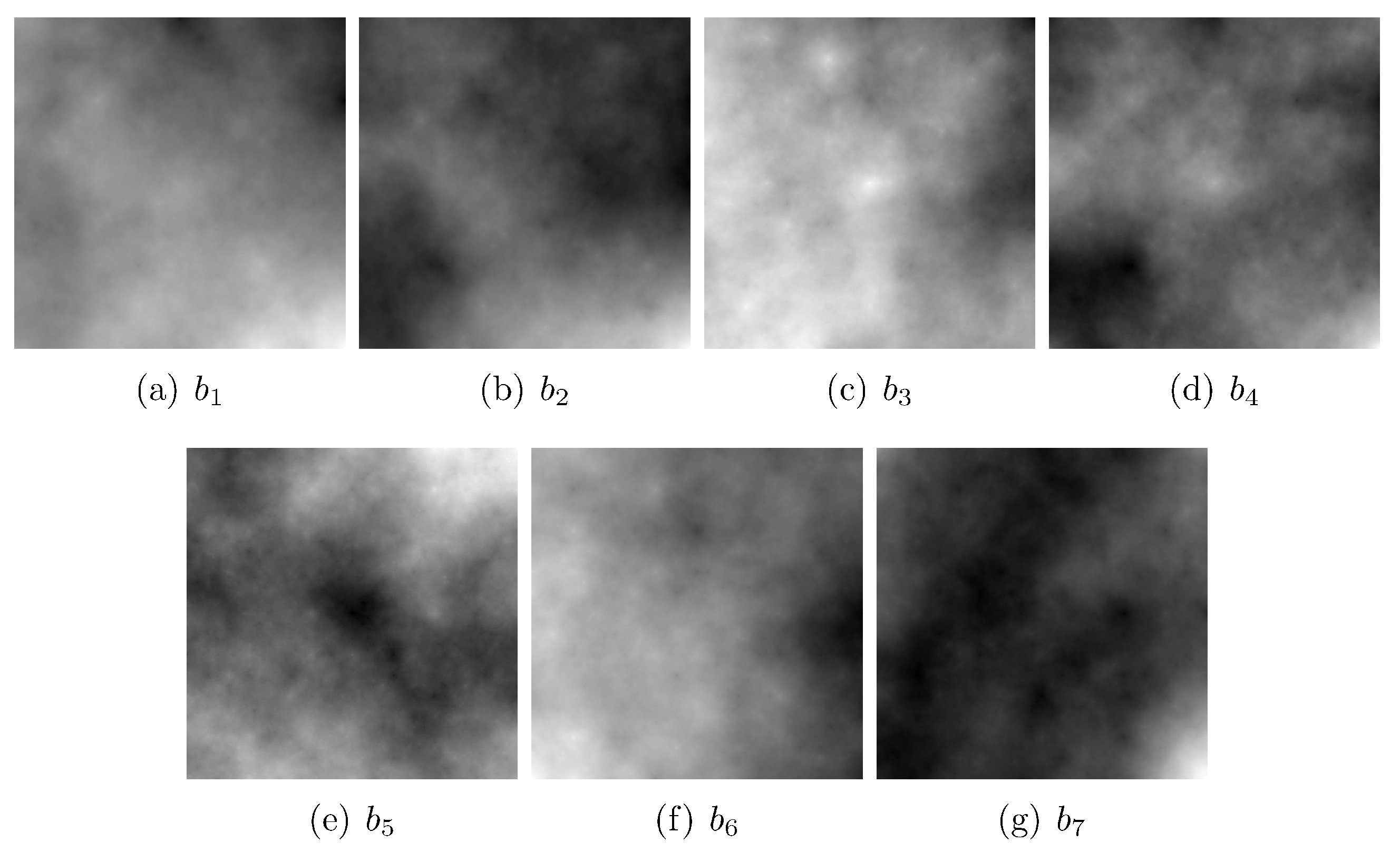
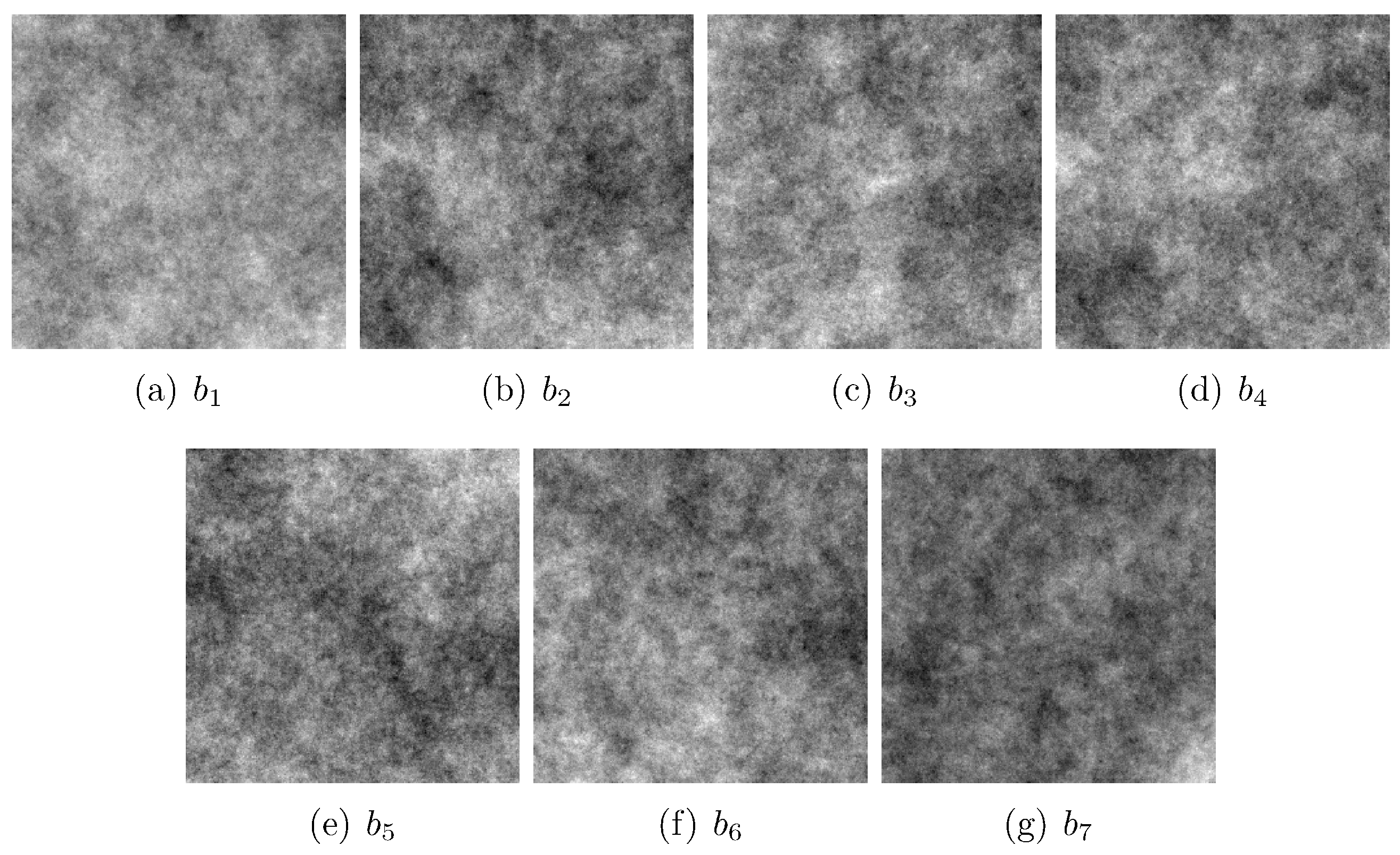
Considering the conclusion in [3], one can extend the proposed approach for the generation of color fractal images to the domain of multi-spectral and perhaps even hyper-spectral fractal images. Consequently, in this paper, we embrace the midpoint displacement algorithm for generating fractal images based on the fractional Brownian motion model. We generated three multi-spectral images of different generated complexities: low generated complexity (), medium generated complexity (), and high generated complexity (). For each of the three complexities, we generated seven statistically independent fractal images using the midpoint displacement approach [2], with each of them corresponding to a wavelength or band in the resulting synthetic multi-spectral image. For the three synthetic fractal multi-spectral images, we chose the following seven wavelengths for the corresponding spectral bands: 450, 500, 550, 600, 650, and 700 nm, all of which are in the visible spectrum. The choice of the wavelengths was completely arbitrary and was performed solely for visualization purposes. In Figure 1, Figure 2 and Figure 3, from (a) to (g), we depict the seven spectral bands () of each of the three generated multi-spectral images. The random seeds used in the generation process were the same for the three multi-spectral images in order to generate similar terrain for the corresponding bands.
The next step is to assign each band in the generated multi-spectral fractal images to a certain wavelength in the visible spectrum. We arbitrarily chose the following mapping between the seven bands of each multi-spectral fractal image (Table 1) in order to produce the actual data cubes corresponding to the synthetic multi-spectral fractal images and, furthermore, to be able to visualize the multi-spectral images (MSIs) as color RGB composite images.
In Figure 4, we show the resulting data cubes for the three generated multi-spectral fractal images (MSFIs) with seven spectral bands. Note that the pseudo coloring of each spectral band channel is used to illustrate the approximate position of the corresponding wavelength on the lambda axis and does not necessarily represent the actual color corresponding to the exact wavelength.
2.3. Visualization of the Multi-Spectral Images
There is a plethora of approaches for the visualization of multi-spectral and hyper-spectral images, and choosing the most appropriate one is not trivial, as the appropriate visualization can be of high importance for the consequent analysis tasks [35]. The existing visualization approaches can be categorized from the simplest band selection to model-based approaches or approaches based on digital image processing techniques and up to more recent methods using machine learning and deep learning paradigms [36].
Band selection consists of a mechanism for choosing three spectral bands from the spectral image and mapping them to the red (R), green (G), and blue (B) channels in the resulting color image. The selection can be performed manually by the user, as in software products such as ENVI [37], or automatically by unsupervised approaches based on the one-bit transform (1BT) [38], normalized information (NI) [39], linear prediction (LP), or minimum end member abundance co-variance methods [40]. Another set of approaches deploys principal component analysis (PCA) for dimensionality reduction of the spectral image data. The straightforward way is to map the first three principal components to the R, G, and B channels of the color image [41]. Other methods use PCA as part of a more complex approach. In [42], an interactive visualization technique based on PCA followed by convex optimization is proposed. In [43], the color RGB image is obtained by fusing the spectral bands with saliency maps obtained before and after applying PCA. In [28], the spectral image is decomposed into two different layers (base and detail) through edge-preserving filtering and dimensionality reduction performed by applying PCA on the base layer and a weighted averaging-based fusion on the detail layer, with the final result being a combination of the two layers. Another set of approaches is based on digital image processing techniques. The authors of [44] used multidimensional scaling followed by detail enhancement using a Laplacian pyramid. The authors of [45] used averaging in order to reduce the number of bands to nine, and then a decolorization algorithm was applied on groups of three adjacent channels, thus producing the final RGB color image. The authors of [46] based their method on t-distributed stochastic neighbor embedding (t-SNE) and bilateral filtering. The work in [47] is also based on bilateral filtering, combined with high-dynamic range processing. The authors of [48] described a pairwise-distance analysis-driven visualization technique.
One approach we embraced for visualization of the generated synthetic multi-spectral images is based on a linear model of color formation proposed in [36]. In this approach, the resulting RGB triplet is obtained by integrating the product of the spectral reflectance curve of each pixel and the spectral sensitivity curve of a camera over the corresponding interval of wavelengths in the visible spectrum. Other linear methods for visualization exist. In [49,50], the RGB values are computed as projections of the hyperspectral pixel values on a particular vector basis, similar to a stretched version of the CIE 1964 color-matching functions, a constant-luma disc basis, or an unwrapped cosine basis.
Another approach we embraced for visualization is the one based on artificial neural networks trained to learn the correspondence between spectral signatures and RGB triplets [36]. Spectral image visualization methods based on machine learning or deep learning usually rely on a pair of matched images: one spectral and one color. The latter one is either obtained through band selection from the spectral image or is independently captured by a different color image sensor. In remote sensing, the two images are registered in order to represent the same geographical area. Such approaches include constrained manifold learning [51], self-organizing maps [52], a moving least squares framework [35], a multi-channel pulse-coupled neural network [53], or convolutional neural networks (CNNs) [54,55].
For each multi-spectral image previously generated, we show in Figure 5, Figure 6 and Figure 7a the color RGB image obtained by using the band selection technique. The wavelengths of 650, 550, and 450 nm were chosen for the R, G, and B channels, respectively, in order to produce the color RGB rendering of the corresponding multi-spectral images. However, displaying a multi-spectral image poses the problem of reducing the potentially large number of bands to just three color RGB channels in order to render the resulting RGB color image on a computer monitor while ensuring that the displayed information was meaningful from the user’s point of view. In Figure 5, Figure 6 and Figure 7b,c, we depict the RGB color images obtained using the linear model and the artificial neural network approaches proposed in [36], respectively. One can observe noticeable differences between the three types of visualization results (including the band selection approach). One reason for this is that the different visualization techniques tend to produce different results, as one can observe in [36]. Another reason is that the resulting multi-spectral pixel values in the generated synthetic fractal images had high variability due to the randomness in the generation mechanism and the statistical independence between bands, which was more than the variability of a natural spectral signature, resulting in the acquisition process of a real scene. Last but not least, in all three cases, the original information, which was richer, was reduced to less information (the dimensionality reduction was from seven spectral bands to only three), and thus more than half of the information was lost in the process of rendering the color RGB composite image.
2.4. Mathematical Proof
Now, for the generated synthetic fractal multi-spectral images, the question is whether they are fractal objects. More concretely, does the variance in the increments result in the generation process obeying the fractal condition? In this section, the generation of multi-spectral fractal images with independent spectral bands is validated mathematically before showing its possible usage in experiments. In [3], it is shown that the resulting color fractal images with three statistically independent color components obey the law of direct proportionality of the variance in the increments. We shall take the same approach for the multi-spectral fractal images with M independent bands.
For an object or signal X having two spatial arguments and M-dimensional vector values (i.e., for the M spectral bands), the variance in the vectorial increments (considering a Euclidean distance between two samples of the signal X) is the following:
By raising the square root to the power of two in Equation (5) and taking into account that the quantities under the square root are positive, one obtains the following expression:
Now, the statistical operator can be distributed to all the M terms regardless of whether they are correlated or not:
By identification, each term represents the marginal variance of the signal X for each spectral band. They should be statistically independent, and each of them, obeying the fractal law in the generation process, assumes a Hurst coefficient that is identical for all spectral bands:
Consequently, the variance of the vectorial increments of the X signal is directly proportional to
which proves that for a multi-spectral image with M statistically-independent spectral bands, the variance of the M-dimensional increments obeys the self-similarity statistical law in Equation (8), thus validating the generation of synthetic multi-spectral images with fractal properties. In conclusion, we analytically showed in Equation (9) that the multi-spectral fractal images with independent spectral bands also obey the fractal law for the generation process. Consequently, they are fractal objects, enabling the estimation of their multi-spectral fractal dimensions.
2.5. Fractal Dimension Estimation for Multi-Spectral Images
We embraced the approach in [27], which allows extending the classical probabilistic box-counting from three color channels to theoretically any number of spectral bands. In order to compute the measure required for the fractal dimension estimation, one has to adopt the analysis boxes for the multi-spectral case. In Figure 8, we show the multi-spectral boxes of sizes , , and for the case of multi-spectral images with two spatial coordinates and spectral bands.
In Figure 9, we depict in blue the vector value of one randomly chosen reddish pixel in the multi-spectral image from Figure 4b, illustrating with light gray the box of size around the pixel’s spectral value. The box size is very often varied from 3 to 41 in steps of 2 (i.e., only the odd-sized boxes for a simpler implementation). For a specific value of , in the estimation of the measure, and for a spectral pixel vector value , the upper and lower parallel covers indicating the limits of the analysis boxes (hyper-cubes) are given by and , respectively.
One question emerging from this experimental set-up regards the pertinence of the embraced fractal model with respect to the generation of multi-spectral images with spectral pixel values corresponding to real spectra. Is the spectral pixel value in Figure 9 a valid spectral signature which could represent a real remotely sensed spectrum from a real scene on the surface of the Earth? To a certain extent, the answer is yes. Given that a reddish pixel was chosen from the lower-right corner of the multi-spectral image in Figure 4b, the shape of the spectral pixel value is pertinent, showing higher values corresponding to the interval corresponding to the red wavelengths. In addition, given the relatively large gaps between spectral bands (i.e., 50 nm), one can assume that the neighbor values in the spectral signature of the pixels are statistically-independent, which is the case in the embraced model. Evidently, for the synthesis of higher-spectral resolution images (such as hyper-spectral images) with fractal properties, this assumption does not stand anymore.
3. Fine-Tuning the Estimator
In order to experimentally test and validate the proposed approach, we considered the three generated multi-spectral fractal data cubes or images with seven spectral bands in Figure 4, having a spatial resolution of pixels, of varying fractal complexity (i.e., low, medium, and high, which translate into Hurst coefficients of , , and , respectively). As we mentioned in the theoretical considerations, the fractal dimension of such a multi-spectral fractal image should comprise between 2 (the complexity of a plane for a uni-image or an image having the same color in every pixel) and 9 (the highest value achievable for a nine-dimensional image (i.e., , with two spatial coordinates plus seven spectral coordinates)). For the three synthetic multi-spectral images, we ran the proposed probabilistic box-counting fractal dimension estimation adapted to the multi-spectral case. The maximum analysis window size was varied for all three images from 41 to 101 in steps of 10. However, the maximum analysis window was set to smaller values for the low- and mid-complexity images, as a maximum window of 31 proved to be very large, especially for the low-complexity image. The threshold for the standard deviation was varied from to in steps of . This standard deviation refers to the extent to which the regression line slope estimation approaches should agree on the measure (represented in a log-log space), which has a direct impact on the fractal dimension estimation. For the three multi-spectral images we obtained the numerical results presented in Table 2, Table 3 and Table 4 for the low, middle and high generated complexity, respectively.
For the lowest-complexity image, the highest achievable fractal dimension was for and for the standard deviation comprised between and . For the mid-complexity image, the highest achievable fractal dimension was for and for the standard deviation comprised between and . It is important to mention the fact that when setting a threshold to such small values, the estimated fractal dimension was estimated based only on three points in the measure. A more reliable estimation would be for and for the standard deviation comprised between and . For the high-complexity image, the highest achievable fractal dimension was for and for the standard deviation comprised between and . Making the same observation as before, a more confident estimation would be for and for the standard deviation comprised between and . As a general observation, the estimated fractal dimensions indicated the correct ranking of the generated image complexity. In addition, as expected, the parameter has to be adapted to the complexity of the image, which in practical application of the fractal estimation approach leads to a paradoxical situation: the fractal dimension which is desired to be estimated and thus unknown should be known in order to set the correct parameter values for the estimator. Another important observation is that, when comparing the current obtained results to the one obtained for color fractal images in [27], the extra information due to the additional four spectral bands, compared with the color RGB case, led to higher complexity values.
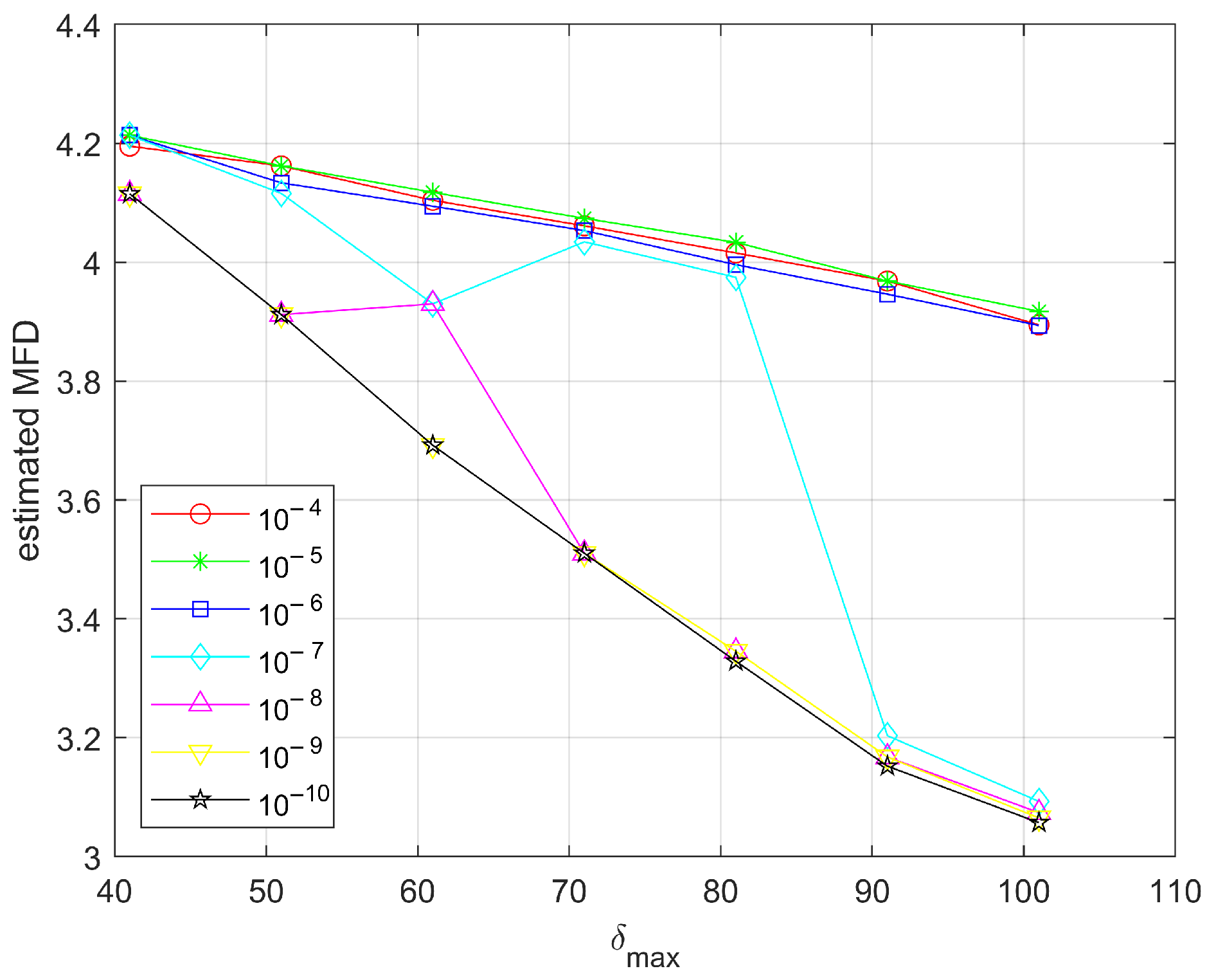
In order to graphically observe the evolution of the estimated multi-spectral fractal dimension, we present the corresponding plots in Figure 10, Figure 11 and Figure 12 (the evolution as a function of ) and Figure 13, Figure 14 and Figure 15 (the evolution as a function of ) for the low, medium and high complexities, respectively, for the common interval of parameter values ( from 41 to 101 and from to ). As a general observation, for the low- and mid-complexity images, the tendency of the estimated multi-spectral fractal dimension was to decrease with the increase in the maximum analysis window and the increase in precision for the agreement of regression line estimators (decrease in the standard deviation). However, this behavior was observed outside the most pertinent interval of values for . A possible explanation for the low performance of the estimator for large values of the maximum analysis box size is the less statistically significant data deployed in the regression line estimation as a consequence of the smaller effective image area for which the fractal analysis was performed (for , approximately 37% of the pixels of the generated images were disregarded). If the image’s spatial resolution (i.e., the image size) allows it, increasing the size of the maximum analysis box makes sense, given that the current estimator disregards the small boxes and allocates more weight to the larger boxes, especially for the high generated complexity fractal images, where the variations of the signals can be very important and thus need to adapt the maximum analysis window. For the high generated complexity image in our experiments, the variation of the analysis box size showed that the middle range of values was the most pertinent one for the estimation. For the appropriate values of , increasing the precision of the slope agreement in the regression line estimators (thus diminishing the standard deviation) clearly improved the estimation, as the estimated multi-spectral fractal dimension increased.
4. Experimental Results
The multi-spectral images used in our experiments were two crops (left upper corner and right lower corner) of a Pavia University hyper-spectral image downsampled in the spectral domain to only seven spectral bands. The Pavia University data set is a 610 × 340 image with a spectral resolution of 4 nm and a spatial resolution of 1.3 m. The image has 103 bands in the 430–860 nm range. The scene in the image contains a total of nine materials according to the provided ground truth, both natural and man-made. We selected 7 spectral bands from the hyper-spectral data: 1, 14, 26, 39, 51, 64, and 76, corresponding to the 430, 482, 530, 582, 630, 682, and 730 nm wavelengths, respectively. We cropped the left upper corner and the right lower corner of the image so that the spatial resolution was pixels, similar to the one of the synthetic fractal images used for validation (see Figure 16 and Figure 17). The estimated multi-spectral fractal dimensions of the seven spectral bands in the Pavia University multi-spectral image crops are presented in Table 5 and Table 6 for varying between 31 and 71 in steps of 10 and varying from to in steps of (i.e., the settings for the most confident estimation results, considering a parameter setting of the estimation tool for low-to-mid-complexity images, as for the considered Pavia University multi-spectral images).
For the left upper corner crop of the Pavia University image, the maximum estimated multi-spectral fractal dimension was , while for the right lower corner crop, it was . The relative difference in complexity was obvious due to the image content; the more complex image contained more colors and variations with more objects present in the scene, while the less complex image contained less colors, less objects, and a larger area of small signal variations. Consequently, the estimator clearly indicates the relative ranking of images as a function of their complexity. However, both images, through their assessed complexities, were in the mid-to-low complexity range.
5. Conclusions
We proposed both a fractal generator and a fractal dimension estimator for multi-spectral images. The proposed estimator allows for fully vector-based fractal analysis of multi-spectral images with fractal properties, compared with all the other existing methods which work only as marginal approaches for each spectral band, considered independently or on color images, thus limiting the application domain and disregarding the rich information in a multi-spectral image. The proposed generator allows for the generation of multi-spectral fractal images with known generated complexity, thus enabling the calibration of the fractal dimension estimator before using it on real-life images in practical use cases.
The generator is based on the midpoint displacement algorithm used for generating fractional Brownian motion, and the estimator is based on the classical probabilistic box-counting approach. The model for the generated multi-spectral fractal images was proven mathematically and illustrated for the case of seven statistically independent spectral bands. The model can be extended theoretically to an arbitrary number of spectral bands, as long as the hypothesis of statistical independence between bands holds (which may not be the case for high spectral resolution images, such as hyper-spectral images). For a qualitative evaluation, the resulting synthetic multi-spectral data sets were visualized as color RGB composites using three different approaches: the widely used band selection, using a linear model for the color formation, and deploying an artificial neural network which was previously trained to learn the correspondences between the multi-spectral pixel signatures and colors specified in the RGB color space. The fractal dimension estimator was adapted to work on nine-dimensional fractal objects, and we estimated the multi-spectral fractal dimension of the generated synthetic multi-spectral fractal images. The estimation requires setting the values for the parameters and , as they should be adapted to the envisaged complexity range of the analyzed images. We presented and interpreted the numerical results obtained in the process of fine-tuning the estimator. However, for the highest generated complexity image, the desirable multi-spectral dimension of has not yet been achieved.
Furthermore, we used the proposed multi-spectral fractal dimension estimator for the fractal complexity assessment of real images. We chose for the experiments the widely known Pavia University hyper-spectral data set, which was first downsampled in the spectral domain from 103 spectral bands to only 7 spectral bands in order to fit to the spectral capabilities of the designed estimator. Secondly, the image was cropped so that the spatial resolution of the resulting images would be identical to one of the generated synthetic multi-spectral fractal images (). The dynamic range was also scaled to the – interval in order to have the same variation of values on all seven bands and in the same range as the spatial domain. The obtained results are in accordance with the perceived complexity of the two scenes. The usefulness of the proposed multi-spectral fractal dimension estimator can be proven in two types of applications: image classification and image segmentation, where the multi-spectral fractal dimension can be used as a global or local feature, respectively, for multi-spectral texture characterization. The proposed model and estimator can be applied on remotely sensed data, such as the multi-spectral images from the Sentinel 2 satellites of the Copernicus Earth Observation program.
6. Future Work
For future work, we identified several questions and possible directions in both fundamental and applied research. One is how to extend the fractal generation model and the fractal dimension estimator to the case of hyper-spectral images, taking into account that the increased spectral resolution imposes considering and modeling the correlation between the spectral bands. Consequently, the assumption made in this article (of statistical independence between spectral bands) does not hold anymore for higher-dimensional cases (with M in the order of hundreds). The second direction is to investigate the possibility of using the fractal dimension estimator for image segmentation and anomaly detection in remotely sensed multi-spectral images. Last but not least, we plan to use the fractal dimension as a local feature for image classification in order to produce an atlas of land cover classes in an Earth observation scenario for agriculture.
Funding
This work was funded by the AI4AGRI project entitled “Romanian Excellence Center on Artificial Intelligence on Earth Observation Data for Agriculture”. The AI4AGRI project received funding from the European Union’s Horizon Europe research and innovation program under grant agreement no. 101079136.
Institutional Review Board Statement
Not applicable.
Informed Consent Statement
Not applicable.
Data Availability Statement
The data is available as open data on the AI4AGRI project website: https://ai4agri.unitbv.ro/ at section Data.
Acknowledgments
The author wishes to thank Noël Richard from University of Poitiers, France, for the fruitful discussions.
Conflicts of Interest
The author declares no conflict of interest.
References
- Mandelbrot, B. The Fractal Geometry of Nature; W.H. Freeman and Co.: New-York, NY, USA, 1982. [Google Scholar]
- Peitgen, H.; Saupe, D. The Sciences of Fractal Images; Springer: Berlin/Heidelberg, Germany, 1988. [Google Scholar]
- Ivanovici, M.; Richard, N. Fractal Dimension of Color Fractal Images. IEEE Trans. Image Process. 2011, 20, 227–235. [Google Scholar] [CrossRef] [PubMed]
- Ivanovici, M. A Fractal Dimension Estimator For Multispectral Images. In Proceedings of the 2022 12th Workshop on Hyperspectral Imaging and Signal Processing: Evolution in Remote Sensing (WHISPERS), Rome, Italy, 13–16 September 2022; pp. 1–4. [Google Scholar]
- Chen, W.; Yuan, S.; Hsiao, H.; Hsieh, C. Algorithms to estimating fractal dimension of textured images. IEEE Int. Conf. Acoust. Speech Signal Process. (ICASSP) 2001, 3, 1541–1544. [Google Scholar]
- Lee, W.; Chen, Y.; Hsieh, K. Ultrasonic liver tissues classification by fractal feature vector based on M-band wavelet transform. IEEE Trans. Med. Imaging 2003, 22, 382–392. [Google Scholar] [CrossRef] [PubMed]
- Ivanovici, M.; Richard, N.; Paulus, D. Color Image Segmentation. In Advanced Color Image Processing and Analysis; Fernandez-Maloigne, C., Ed.; Springer: New York, NY, USA, 2013; Chapter 8; pp. 219–277. [Google Scholar]
- Wang, W.; Wang, W.; Hu, Z. Retinal vessel segmentation approach based on corrected morphological transformation and fractal dimension. IET Image Process. 2019, 13, 2538–2547. [Google Scholar] [CrossRef]
- Shahrezaei, I.; Kim, H. Fractal Analysis and Texture Classification of High-Frequency Multiplicative Noise in SAR Sea-Ice Images Based on a Transform- Domain Image Decomposition Method. IEEE Access 2020, 8, 40198–40223. [Google Scholar] [CrossRef]
- Wu, L.; Liu, X.; Qin, Q.; Zhao, B.; Ma, Y.; Liu, M.; Jiang, T. Scaling Correction of Remotely Sensed Leaf Area Index for Farmland Landscape Pattern With Multitype Spatial Heterogeneities Using Fractal Dimension and Contextural Parameters. IEEE J. Sel. Top. Appl. Earth Obs. Remote Sens. 2018, 11, 1472–1481. [Google Scholar] [CrossRef]
- Hausdorff, F. Dimension und äußeres Maß. Math. Ann. 1918, 79, 157–179. [Google Scholar] [CrossRef]
- Voss, R. Random Fractals: Characterization and measurement. Scaling Phenom. Disord. Syst. 1986, 10, 51–61. [Google Scholar] [CrossRef]
- Keller, J.; Chen, S. Texture Description and segmentation through Fractal Geometry. Comput. Vis. Graph. Image Process. 1989, 45, 150–166. [Google Scholar] [CrossRef]
- Falconer, K. Fractal Geometry, Mathematical Foundations and Applications; John Wiley and Sons: Hoboken, NJ, USA, 1990. [Google Scholar]
- Maragos, P.; Sun, F. Measuring the fractal dimension of signals: Morphological covers and iterative optimization. IEEE Trans. Signal Process. 1993, 41, 108–121. [Google Scholar] [CrossRef]
- Allain, C.; Cloitre, M. Characterizing the lacunarity of random and deterministic fractal sets. Phys. Rev. A 1991, 44, 3552–3558. [Google Scholar] [CrossRef]
- Castillo, O.; Melin, P. A New Method for Fuzzy Estimation of the Fractal Dimension and its Applications to Time Series Analysis and Pattern Recognition. In Proceedings of the Fuzzy Information Processing Society, 2000, NAFIPS, 19th International Conference of the North American, Atlanta, GA, USA, 13–15 July 2000; pp. 451–455. [Google Scholar]
- Pedrycz, W.; Bargiela, A. Fuzzy fractal dimensions and fuzzy modeling. Inf. Sci. 2003, 153, 199–216. [Google Scholar] [CrossRef]
- Aiazzi, B.; Alparone, L.; Baronti, S.; Bulletti, A.; Garzelli, A. Robust Estimation of Image Fractal Dimension based on Pyramidal Decomposition. In Proceedings of the 6th IEEE International Conference on Electronic, Circuits ans Systems, Paphos, Cyprus, 5–8 September 1999; Volume 1, pp. 553–556. [Google Scholar]
- Jansson, S. Evaluation of Methods for Estimating Fractal Properties of Intensity Images. Ph.D. Thesis, Umea University, Umea, Sweden, 2006. [Google Scholar]
- Sun, W.; Xu, G.; Gong, P.; Liang, S. Fractal analysis of remotely sensed images: A review of methods and applications. Int. J. Remote Sens. 2006, 27, 4963–4990. [Google Scholar] [CrossRef]
- Kinsner, W. A unified approach to fractal dimensions. In Proceedings of the 4th IEEE International Conference on Cognitive Informatics, Irvine, CA, USA, 8–10 August 2005; pp. 58–72. [Google Scholar]
- Manousaki, A.; Manios, A.; Tsompanaki, E.; Tosca, A. Use of color texture in determining the nature of melanocytic skin lesions—A qualitative and quantitative approach. Comput. Biol. Med. 2006, 36, 416–427. [Google Scholar] [CrossRef] [PubMed]
- Ivanovici, M.; Richard, N. Entropy versus fractal complexity for computer-generated color fractal images. In Proceedings of the 4th CIE Expert Symposium on Colour and Visual Appearance, Prague, Czech Republic, 6–7 September 2016. [Google Scholar]
- Zhao, X.; Wang, X. An Approach to Compute Fractal Dimension of Color Images. Fractals 2017, 25, 1750007. [Google Scholar] [CrossRef]
- Nayak, S.; Mishra, J.; Palai, G. An extended DBC approach by using maximum Euclidian distance for fractal dimension of color images. Optik 2018, 166, 110–115. [Google Scholar] [CrossRef]
- Ivanovici, M. Fractal Dimension of Color Fractal Images With Correlated Color Components. IEEE Trans. Image Process. 2020, 29, 8069–8082. [Google Scholar] [CrossRef]
- Kang, X.; Duan, P.; Li, S. Hyperspectral image visualization with edge-preserving filtering and principal component analysis. Inf. Fusion 2020, 57, 130–143. [Google Scholar] [CrossRef]
- Teke, M.; Deveci, H.S.; Haliloğlu, O.; Gürbüz, S.Z.; Sakarya, U. A short survey of hyperspectral remote sensing applications in agriculture. In Proceedings of the 2013 6th International Conference on Recent Advances in Space Technologies (RAST), Istanbul, Turkey, 12–14 June 2013; pp. 171–176. [Google Scholar]
- Reshma, S.; Veni, S. Comparative analysis of classification techniques for crop classification using airborne hyperspectral data. In Proceedings of the 2017 International Conference on Wireless Communications, Signal Processing and Networking (WiSPNET), Chennai, India, 22–24 March 2017; pp. 2272–2276. [Google Scholar]
- Piiroinen, R.; Heiskanen, J.; Maeda, E.; Viinikka, A.; Pellikka, P. Classification of tree species in a diverse African agroforestry landscape using imaging spectroscopy and laser scanning. Remote Sens. 2017, 9, 875. [Google Scholar] [CrossRef] [Green Version]
- Fricker, G.A.; Ventura, J.D.; Wolf, J.A.; North, M.P.; Davis, F.W.; Franklin, J. A convolutional neural network classifier identifies tree species in mixed-conifer forest from hyperspectral imagery. Remote Sens. 2019, 11, 2326. [Google Scholar] [CrossRef] [Green Version]
- Dumke, I.; Nornes, S.M.; Purser, A.; Marcon, Y.; Ludvigsen, M.; Ellefmo, S.L.; Johnsen, G.; Søreide, F. First hyperspectral imaging survey of the deep seafloor: High-resolution mapping of manganese nodules. Remote Sens. Environ. 2018, 209, 19–30. [Google Scholar] [CrossRef]
- Acosta, I.C.C.; Khodadadzadeh, M.; Tusa, L.; Ghamisi, P.; Gloaguen, R. A machine learning framework for drill-core mineral mapping using hyperspectral and high-resolution mineralogical data fusion. IEEE J. Sel. Top. Appl. Earth Obs. Remote Sens. 2019, 12, 4829–4842. [Google Scholar] [CrossRef]
- Liao, D.; Chen, S.; Qian, Y. Visualization of Hyperspectral Images Using Moving Least Squares. In Proceedings of the 2018 24th International Conference on Pattern Recognition (ICPR), Beijing, China, 20–24 August 2018; pp. 2851–2856. [Google Scholar]
- Coliban, R.M.; Marincaş, M.; Hatfaludi, C.; Ivanovici, M. Linear and Non-Linear Models for Remotely-Sensed Hyperspectral Image Visualization. Remote Sens. 2020, 12, 2479. [Google Scholar] [CrossRef]
- Process and Analyze All Types of Imagery and Data. Available online: https://www.harrisgeospatial.com/Software-Technology/ENVI/ (accessed on 21 January 2023).
- Demir, B.; Celebi, A.; Erturk, S. A low-complexity approach for the color display of hyperspectral remote-sensing images using one-bit-transform-based band selection. IEEE Trans. Geosci. Remote Sens. 2008, 47, 97–105. [Google Scholar] [CrossRef]
- Le Moan, S.; Mansouri, A.; Voisin, Y.; Hardeberg, J.Y. A constrained band selection method based on information measures for spectral image color visualization. IEEE Trans. Geosci. Remote Sens. 2011, 49, 5104–5115. [Google Scholar] [CrossRef] [Green Version]
- Su, H.; Du, Q.; Du, P. Hyperspectral imagery visualization using band selection. In Proceedings of the 2012 4th Workshop on Hyperspectral Image and Signal Processing: Evolution in Remote Sensing (WHISPERS), Shanghai, China, 4–7 June 2012; pp. 1–4. [Google Scholar]
- Tyo, J.S.; Konsolakis, A.; Diersen, D.I.; Olsen, R.C. Principal-components-based display strategy for spectral imagery. IEEE Trans. Geosci. Remote Sens. 2003, 41, 708–718. [Google Scholar] [CrossRef] [Green Version]
- Cui, M.; Razdan, A.; Hu, J.; Wonka, P. Interactive hyperspectral image visualization using convex optimization. IEEE Trans. Geosci. Remote Sens. 2009, 47, 1673–1684. [Google Scholar]
- Khan, H.A.; Khan, M.M.; Khurshid, K.; Chanussot, J. Saliency based visualization of hyper-spectral images. In Proceedings of the 2015 IEEE International Geoscience and Remote Sensing Symposium (IGARSS), Milan, Italy, 26–31 July 2015; pp. 1096–1099. [Google Scholar]
- Fang, J.; Qian, Y. Local detail enhanced hyperspectral image visualization. In Proceedings of the 2015 IEEE International Geoscience and Remote Sensing Symposium (IGARSS), Milan, Italy, 26–31 July 2015; pp. 1092–1095. [Google Scholar]
- Kang, X.; Duan, P.; Li, S.; Benediktsson, J.A. Decolorization-based hyperspectral image visualization. IEEE Trans. Geosci. Remote Sens. 2018, 56, 4346–4360. [Google Scholar] [CrossRef]
- Zhang, B.; Yu, X. Hyperspectral image visualization using t-distributed stochastic neighbor embedding. In Proceedings of the MIPPR 2015: Remote Sensing Image Processing, Geographic Information Systems, and Other Applications, Enshi, China, 31 October–1 November 2015; Liu, J., Sun, H., Eds.; International Society for Optics and Photonics, SPIE: Bellingham, WA, USA, 2015; Volume 9815, pp. 14–21. [Google Scholar]
- Ertürk, S.; Süer, S.; Koç, H. A high-dynamic-range-based approach for the display of hyperspectral images. IEEE Geosci. Remote Sens. Lett. 2014, 11, 2001–2004. [Google Scholar] [CrossRef]
- Long, Y.; Li, H.C.; Celik, T.; Longbotham, N.; Emery, W.J. Pairwise-Distance-Analysis-Driven Dimensionality Reduction Model with Double Mappings for Hyperspectral Image Visualization. Remote Sens. 2015, 7, 7785–7808. [Google Scholar] [CrossRef] [Green Version]
- Jacobson, N.P.; Gupta, M.R. Design goals and solutions for display of hyperspectral images. IEEE Trans. Geosci. Remote Sens. 2005, 43, 2684–2692. [Google Scholar] [CrossRef]
- Jacobson, N.P.; Gupta, M.R.; Cole, J.B. Linear fusion of image sets for display. IEEE Trans. Geosci. Remote Sens. 2007, 45, 3277–3288. [Google Scholar] [CrossRef]
- Liao, D.; Qian, Y.; Tang, Y.Y. Constrained manifold learning for hyperspectral imagery visualization. IEEE J. Sel. Top. Appl. Earth Obs. Remote Sens. 2018, 11, 1213–1226. [Google Scholar] [CrossRef] [Green Version]
- Jordan, J.; Angelopoulou, E. Hyperspectral image visualization with a 3-D self-organizing map. In Proceedings of the 2013 5th Workshop on Hyperspectral Image and Signal Processing: Evolution in Remote Sensing (WHISPERS), Gainesville, FL, USA, 26–28 June 2013; pp. 1–4. [Google Scholar]
- Duan, P.; Kang, X.; Li, S.; Ghamisi, P. Multichannel pulse-coupled neural network-based hyperspectral image visualization. IEEE Trans. Geosci. Remote Sens. 2019, 58, 2444–2456. [Google Scholar] [CrossRef]
- Duan, P.; Kang, X.; Li, S. Convolutional Neural Network for Natural Color Visualization of Hyperspectral Images. In Proceedings of the IGARSS 2019—2019 IEEE International Geoscience and Remote Sensing Symposium, Yokohama, Japan, 28 July–2 August 2019; pp. 3372–3375. [Google Scholar]
- Tang, R.; Liu, H.; Wei, J.; Tang, W. Supervised learning with convolutional neural networks for hyperspectral visualization. Remote Sens. Lett. 2020, 11, 363–372. [Google Scholar] [CrossRef]
Figure 1.
The seven spectral bands of the MSI with low generated complexity ().

Figure 2.
The seven spectral bands of the MSI with medium generated complexity ().

Figure 3.
The sevenspectral bands of the MSI with high generated complexity ().

Figure 4.
The multi-spectral fractal image data cubes.

Figure 5.
The RGB color composite images of the MSFI in Figure 4a.
Figure 5.
The RGB color composite images of the MSFI in Figure 4a.

Figure 6.
The RGB color composite images of the MSFI in Figure 4b.
Figure 6.
The RGB color composite images of the MSFI in Figure 4b.

Figure 7.
The RGB color composite images of the MSFI in Figure 4c.
Figure 7.
The RGB color composite images of the MSFI in Figure 4c.

Figure 8.
The analysis boxes for sizes , , and .

Figure 9.
One pixel value (in blue) and the corresponding area between the -parallel covers (for ).

Figure 10.
The estimated multi-spectral fractal dimension as a function of for the low generated complexity () multi-spectral fractal image.
Figure 10.
The estimated multi-spectral fractal dimension as a function of for the low generated complexity () multi-spectral fractal image.

Figure 11.
The estimated multi-spectral fractal dimension as a function of for the medium generated complexity () multi-spectral fractal image.
Figure 11.
The estimated multi-spectral fractal dimension as a function of for the medium generated complexity () multi-spectral fractal image.

Figure 12.
The estimated multi-spectral fractal dimension as a function of for the high generated complexity () multi-spectral fractal image.
Figure 12.
The estimated multi-spectral fractal dimension as a function of for the high generated complexity () multi-spectral fractal image.

Figure 13.
The estimated multi-spectral fractal dimension as a function of for the low generated complexity () multi-spectral fractal image.
Figure 13.
The estimated multi-spectral fractal dimension as a function of for the low generated complexity () multi-spectral fractal image.

Figure 14.
The estimated multi-spectral fractal dimension as a function of for the medium generated complexity () multi-spectral fractal image.
Figure 14.
The estimated multi-spectral fractal dimension as a function of for the medium generated complexity () multi-spectral fractal image.

Figure 15.
The estimated multi-spectral fractal dimension as a function of for the high generated complexity () multi-spectral fractal image.
Figure 15.
The estimated multi-spectral fractal dimension as a function of for the high generated complexity () multi-spectral fractal image.

Figure 16.
The seven spectral bands of the Pavia University MSI and the correponding band selection (10, 31, and 46) color RGB image for the Pavia University hyperspectral data set (left upper corner).
Figure 16.
The seven spectral bands of the Pavia University MSI and the correponding band selection (10, 31, and 46) color RGB image for the Pavia University hyperspectral data set (left upper corner).

Figure 17.
The seven spectral bands of the Pavia University MSI and the correponding band selection (10, 31, and 46) color RGB image for the Pavia University hyperspectral data set (right lower corner).
Figure 17.
The seven spectral bands of the Pavia University MSI and the correponding band selection (10, 31, and 46) color RGB image for the Pavia University hyperspectral data set (right lower corner).


Table 1.
The arbitrary mapping between the seven generated bands and the corresponding wavelengths.
| 400 nm | 450 nm | 500 nm | 550 nm | 600 nm | 650 nm | 700 nm |
Table 2.
The estimated multi-spectral fractal dimension (MFD) of multi-spectral fractal image with low generated complexity ().
Table 2.
The estimated multi-spectral fractal dimension (MFD) of multi-spectral fractal image with low generated complexity ().
| 7 | 2.2727 | 2.2727 | 2.2727 | 2.2727 | 2.2727 | 2.2727 | 2.2727 | |
| 11 | 2.4790 | 2.7653 | 2.7653 | 2.7653 | 2.7653 | 2.6934 | 2.6934 | |
| 21 | 2.5873 | 2.5578 | 2.5411 | 2.5308 | 2.5268 | 2.5268 | 2.5257 | |
| 31 | 2.5393 | 2.5134 | 2.5134 | 2.5134 | 2.5083 | 2.5083 | 2.4816 | |
| 41 | 2.5233 | 2.5065 | 2.5013 | 2.4965 | 2.4755 | 2.4755 | 2.4733 | |
| 51 | 2.5014 | 2.4893 | 2.4839 | 2.4604 | 2.4574 | 2.4394 | 2.4394 | |
| 61 | 2.4903 | 2.4786 | 2.4533 | 2.4471 | 2.4443 | 2.4164 | 2.4080 | |
| 71 | 2.4702 | 2.4625 | 2.4468 | 2.4439 | 2.4414 | 2.4320 | 2.4214 | |
| 81 | 2.4693 | 2.4613 | 2.4539 | 2.4473 | 2.4302 | 2.4269 | 2.4269 | |
| 91 | 2.4773 | 2.4606 | 2.4469 | 2.4391 | 2.4321 | 2.3607 | 2.3651 | |
| 101 | 2.4695 | 2.4397 | 2.4165 | 2.3596 | 2.3587 | 2.3587 | 2.3579 | |
Table 3.
The estimated multi-spectral fractal dimension (MFD) of multi-spectral fractal image with medium generated complexity ().
Table 3.
The estimated multi-spectral fractal dimension (MFD) of multi-spectral fractal image with medium generated complexity ().
| 21 | 3.5975 | 3.8173 | 3.8173 | 3.9665 | 3.9665 | 3.9665 | 3.9665 | |
| 31 | 4.1713 | 4.1713 | 4.2113 | 4.2113 | 4.2229 | 4.2229 | 4.2229 | |
| 41 | 4.1952 | 4.2133 | 4.2133 | 4.2133 | 4.1150 | 4.1150 | 4.1150 | |
| 51 | 4.1619 | 4.1619 | 4.1334 | 4.1157 | 3.9118 | 3.9118 | 3.9118 | |
| 61 | 4.1040 | 4.1175 | 4.0941 | 3.9299 | 3.9299 | 3.6920 | 3.6920 | |
| 71 | 4.0611 | 4.0737 | 4.0531 | 4.0342 | 3.5104 | 3.5104 | 3.5104 | |
| 81 | 4.0154 | 4.0333 | 3.9957 | 3.9744 | 3.3457 | 3.3457 | 3.3287 | |
| 91 | 3.9682 | 3.9682 | 3.9462 | 3.2035 | 3.1677 | 3.1677 | 3.1523 | |
| 101 | 3.8944 | 3.9172 | 3.8935 | 3.0930 | 3.0742 | 3.0652 | 3.0572 | |
Table 4.
The estimated multi-spectral fractal dimension (MFD) of multi-spectral fractal image with high generated complexity ().
Table 4.
The estimated multi-spectral fractal dimension (MFD) of multi-spectral fractal image with high generated complexity ().
| 41 | 0.7523 | 1.1958 | 4.5693 | 5.1281 | 5.1281 | 5.1281 | 5.1281 | |
| 51 | 5.4481 | 5.8568 | 5.9662 | 5.9662 | 5.9662 | 5.9662 | 5.9662 | |
| 61 | 5.7691 | 6.0965 | 6.4867 | 6.4867 | 6.4867 | 6.4867 | 6.4867 | |
| 71 | 6.1941 | 6.5484 | 6.6172 | 6.6555 | 6.6555 | 6.6555 | 6.6555 | |
| 81 | 6.5319 | 6.5319 | 6.5089 | 6.3486 | 6.3486 | 6.1297 | 6.1297 | |
| 91 | 6.4054 | 6.4419 | 6.4574 | 6.4574 | 6.6636 | 6.6636 | 6.6636 | |
| 101 | 6.3180 | 5.7551 | 5.2170 | 5.2170 | 5.0599 | 5.0599 | 5.0599 | |
Table 5.
The estimated multi-spectral fractal dimension (MFD) of the Pavia University multi-spectral image (left upper corner).
Table 5.
The estimated multi-spectral fractal dimension (MFD) of the Pavia University multi-spectral image (left upper corner).
| 31 | 3.2891 | 3.3425 | 3.4251 | 3.4876 | 3.5405 | |
| 41 | 3.4330 | 3.5144 | 3.4140 | 3.4140 | 3.4140 | |
| 51 | 3.4891 | 3.5072 | 3.5072 | 3.2730 | 3.2730 | |
| 61 | 3.3639 | 3.3863 | 3.3595 | 3.3595 | 3.0681 | |
| 71 | 3.2634 | 3.2879 | 3.2879 | 2.4161 | 2.4161 | |
Table 6.
The estimated multi-spectral fractal dimension (MFD) of the Pavia University multi-spectral image (right lower corner).
Table 6.
The estimated multi-spectral fractal dimension (MFD) of the Pavia University multi-spectral image (right lower corner).
| 11 | 0.9443 | 1.4164 | 1.4164 | 1.4164 | 1.7307 | |
| 21 | 2.7358 | 2.9679 | 2.9679 | 3.0386 | 3.0386 | |
| 31 | 3.0320 | 3.0320 | 3.0456 | 3.0456 | 2.9699 | |
| 41 | 2.9221 | 2.9221 | 2.7059 | 2.6599 | 2.6599 | |
| 51 | 2.8264 | 2.8264 | 2.8324 | 2.5104 | 2.5464 | |
Disclaimer/Publisher’s Note: The statements, opinions and data contained in all publications are solely those of the individual author(s) and contributor(s) and not of MDPI and/or the editor(s). MDPI and/or the editor(s) disclaim responsibility for any injury to people or property resulting from any ideas, methods, instructions or products referred to in the content. |
© 2023 by the author. Licensee MDPI, Basel, Switzerland. This article is an open access article distributed under the terms and conditions of the Creative Commons Attribution (CC BY) license (https://creativecommons.org/licenses/by/4.0/).
Share and Cite
MDPI and ACS Style
Ivanovici, M. A Multi-Spectral Fractal Image Model and Its Associated Fractal Dimension Estimator. Fractal Fract. 2023, 7, 238. https://doi.org/10.3390/fractalfract7030238
AMA Style
Ivanovici M. A Multi-Spectral Fractal Image Model and Its Associated Fractal Dimension Estimator. Fractal and Fractional. 2023; 7(3):238. https://doi.org/10.3390/fractalfract7030238
Chicago/Turabian StyleIvanovici, Mihai. 2023. "A Multi-Spectral Fractal Image Model and Its Associated Fractal Dimension Estimator" Fractal and Fractional 7, no. 3: 238. https://doi.org/10.3390/fractalfract7030238