Article

First-of-Its-Kind Frequency Enhancement Methodology Based on an Optimized Combination of FLC and TFOIDFF Controllers Evaluated on EVs, SMES, and UPFC-Integrated Smart Grid

1
Department of Electrical and Computer Engineering, Faculty of Engineering, King Abdulaziz University, Jeddah 21589, Saudi Arabia
2
Department of Electrical Engineering, University of Business and Technology, Ar Rawdah, Jeddah 23435, Saudi Arabia
3
Department of Electrical Power and Machines, Faculty of Engineering, Alexandria University, Alexandria 21544, Egypt
*
Author to whom correspondence should be addressed.
Fractal Fract. 2023, 7(11), 807; https://doi.org/10.3390/fractalfract7110807
Submission received: 22 October 2023 / Revised: 2 November 2023 / Accepted: 4 November 2023 / Published: 6 November 2023

Abstract

:
The most recent advancements in renewable energy resources, as well as their broad acceptance in power sectors, have created substantial operational, security, and management concerns. As a result of the continual decrease in power system inertia, it is critical to maintain the normal operating frequency and reduce tie-line power changes. The preceding issues sparked this research, which proposes the Fuzzy Tilted Fractional Order Integral Derivative with Fractional Filter (FTFOIDFF), a unique load frequency controller. The FTFOIDFF controller described here combines the benefits of tilt, fuzzy logic, FOPID, and fractional filter controllers. Furthermore, the prairie dog optimizer (PDO), a newly developed metaheuristic optimization approach, is shown to efficiently tune the suggested controller settings as well as the forms of the fuzzy logic membership functions in the two-area hybrid power grid investigated in this paper. When the PDO results are compared to those of the Seagull Optimization Algorithm, the Runge Kutta optimizer, and the Chaos Game Optimizer for the same hybrid power system, PDO prevails. The system model incorporates physical constraints such as communication time delays and generation rate constraints. In addition, a unified power flow controller (UPFC) is put in the tie-line, and SMES units have been planned in both regions. Furthermore, the contribution of electric vehicles (EVs) is considered in both sections. The proposed PDO-based FTFOIDFF controller outperformed many PDO-based traditional (such as proportional integral derivative (PID), proportional integral derivative acceleration (PIDA), and TFOIDFF) and intelligent (such as Fuzzy PID and Fuzzy PIDA) controllers from the literature. The suggested PDO-based FTFOIDFF controller has excellent performance due to the usage of various load patterns such as step load perturbation, multi-step load perturbation, random load perturbation, random sinusoidal load perturbation, and pulse load perturbation. Furthermore, a variety of scenarios have been implemented to demonstrate the advantageous effects that SMES, UPFC, and EV units have on the overall performance of the system. The sensitivity of a system is ascertained by modifying its parameters from their standard configurations. According to the simulation results, the suggested PDO-based FTFOIDFF controller can improve system stability despite the multiple difficult conditions indicated previously. According to the MATLAB/Simulink data, the proposed method decreased the total fitness function to 0.0875, representing a 97.35% improvement over PID, 95.84% improvement over PIDA, 92.45% improvement over TFOIDFF, 83.43% improvement over Fuzzy PID, and 37.9% improvement over Fuzzy PIDA.

1. Introduction

1.1. Motivation and Incitement

The provision of a continuous supply of electrical power of a quality that is deemed satisfactory to each and every customer inside a power system should be the primary goal of any power system utility. The electric grid will be in equilibrium when there is a balance between the quantity of electrical power that is needed and the amount that is generated. To obtain a desirable profile of voltage (reactive power balance) and desirable frequency ranges (actual power balance), two basic control strategies are used. The first is known as an automatic voltage regulator (AVR), while the second can either be referred to as an automatic generation control (AGC) or a load frequency controller (LFC) [1]. In a power system that is linked, the objective of LFC is to minimize the transient variations in area frequency and tie-line power exchange while also ensuring that their steady-state errors are zero [2]. Induction motors and transformers are susceptible to experiencing increased magnetizing currents if the frequency experiences a significant dip. The widespread usage of electric clocks and the use of frequency for many other timing applications both necessitate the correct preservation of synchronous time, which must be proportional to frequency and must also incorporate the integral of that variable. The loads are shifted about in a haphazard and fleeting manner by the consumers of electric power. As a direct consequence of this, mismatches between generation and load occur all of a sudden. Due to the mismatch, power is pulled from or fed into the rotor, which results in a change in the generator speed and, as a consequence, the frequency of the system (since frequency is strongly connected to the generator speed). Without proper control, it is difficult to keep the generation and load balances in the correct proportions. Therefore, a control mechanism is needed to mitigate the effects of unpredictable shifts in load and to keep the frequency at the required value. Continuously regulating the active power output of the generator in order to correspond with the randomly variable load is the responsibility of the Load frequency control loop [3].
In a power system that is practically integrated, the generation often consists of a mix of several types of power generation, including thermal, hydro, nuclear, and gas. Nevertheless, due to the tremendous efficiency of nuclear facilities, they are often maintained at a base load that is rather near to their maximum output. The generation of electricity from gas is ideally suited for addressing the varied load demand. Consequently, gas plants are only utilised to satisfy peak demand [4,5]. Therefore, traditional nonrenewable resources were the most common kind of installation in the energy industry. Worries are shifting, however, away from these sources of electricity due to their scarcity and the negative effects they have on the environment [6]. These worries centre on the installation of sources of power that are based on renewable energy. Therefore, a greater emphasis must be placed on sustainable development in order to replace non-renewable sources with renewable energy sources (RESs), such as wind generation, solar photovoltaic (PV) generation, bio-diesel production, and so on. In addition, the improvement of power grids that are based on RES by making use of energy storage devices, the cooperative functioning of electric vehicles (EVs) that have been installed, and other similar activities have garnered significant interest from researchers, industry, and government laws and incentives. They have the potential to contribute to the maintenance of power networks’ resilience and dependability [7]. In addition, an improvement in the overall efficiency of power grids is attainable by utilizing modern single- and multi-objective optimisation techniques, such as the robust optimisation methods [8] and the stochastic optimisation methods [9].

1.2. Literature Review

Intermittency, inconstant loading profiles, lower inertia, and other issues are only some of the obstacles that power systems based on RES must contend with. The connectivity of electricity grids that are powered by RES is beneficial in a number of different ways. Nevertheless, renewable energy sources (RES) contribute to the development of fragile power networks that have an unstable reaction to disturbance [10]. When compared to typical grids based on non-renewable sources of energy, renewable-based grids have a far lower inertial response, which is the primary cause of grid instability. Since PV and wind generation are coupled with power interface converters, they are unable to withstand a considerable inertial response, which restricts their capacity for balancing power needs [11]. A low inertial response causes significant instability in power grids, which reduces the controllability of frequency deviations in power grids that are based on RES [12]. This instability may be mitigated by increasing the penetration level of RES.
When the governor system is incapable to cope with frequency changes owing to its slow reaction, active power sources with rapid reactions, such (SMES), are very beneficial in boosting the responsiveness of a system [13,14]. The efficiency of tiny (MES) units, including superconducting and conventional loss varieties, for load frequency regulation is investigated in [15]. There are suggestions on how to make the most of these units’ limited energy storage capacity in order to improve the responsiveness of extensive power systems. Since the SMES unit is capable of simultaneously managing both active and reactive powers [16], it is one of the most powerful and critical stabilizers of frequency oscillations. This is due to the fact that frequency oscillations may be quite dangerous. There have been reports in the published literature [17,18] that discuss the practicability of using SMES to improve load frequency performance. Recent developments in power electronics have resulted in the creation of controllers known as flexible alternating current transmission systems (FACTS), which are used in power systems. The performance of a power system can be improved by utilizing FACTS controllers due to their ability to quickly manage the state of the network and their potential to be utilised in this capacity. The FACTS family includes the unified power flow controller (UPFC), which has several characteristics that may be used in a variety of contexts. In addition to managing the UPFC bus voltage and shunt reactive power, UPFC, which comprises of a series and shunt converter coupled by a common dc link capacitor, can also regulate the actual and active power flow in transmission lines [19]. This is made possible by the fact that UPFC is constructed from a series and shunt converter. It has been observed in the literature [20,21] that the effect of various FACTS controllers, such as static synchronous series compensator (SSSC) and thyristor controlled phase shifter (TCPS), working in conjunction with SMES for AGC can have a significant influence. In light of the aforementioned, the LFC analysis presented in this work was carried out while SMES and UPFC were also present.
Power grids that are based on RES have the potential to improve their overall performance if improved and optimized control mechanisms are used [22,23]. LFC has seen widespread adoption as a solution to the frequency variation issues plaguing power networks that are based on RES. The control of generated power is the responsibility of LFCs in order to mitigate loading variations, incompatible parameters, the changing nature of RESs, disruptions, and other similar occurrences [24]. The resistance of power grids to disturbances is directly proportional to the kind of LFC method that is put into practice. In addition, the power grid responsiveness as well as the complexity of the design process are both determined by the correct optimal LFC design technique [25].
For the purpose of load frequency regulation in power systems, a variety of control structures have been discussed and described in the aforementioned literature. First, standard integral order controllers such as PI and PID controllers, which are known for their ease of use, have been adapted for use as load frequency controllers [26]. As a direct consequence of this, soft computing technologies have been included into the process of tuning various controllers. Multiple optimisation strategies, such as particle swarm optimisation [27], whale optimisation algorithm [28], cuckoo search algorithm [29], marine predators algorithm [30], sine cosine adopted dingo optimisation algorithm [31], colliding bodies optimizer [32], cohort intelligence optimization [33], and sea horse optimizer [34] have been used to the design of LFC in order to conduct more research and development on the technology. Using PID controllers, several LFC strategies have been suggested as potential solutions for multi-area linked power systems. These methodologies were important contributors to the preliminary phase of the deregulated LFC operation. Contrarily, it has been noticed that the majority of research have focused their emphasis on LFC difficulties unique to the conventional power system. Furthermore, the significant penetration of RES may bring up a number of challenges, such as voltage instability, poor power quality, frequency variation, and reliability issues.
Regrettably, traditional PID controllers have a number of shortcomings when it comes to coping with system uncertainties such as the fluctuation of RES [35]. As a result, various adjustments have been made in order to enhance the functionality of conventional PID controllers such as the tilt-integral derivative (TID) and the (FOPID) controllers. These improvements have been made in order to increase performance. Calculus using fractions serves as the foundation for these controllers [36]. The efficacy of fractional controllers has been demonstrated by the empirical investigations conducted by researchers [37,38,39], whereby they have applied mathematical principles to actual scenarios. Several other methods of optimization, including as the differential evolution algorithm [40] and the performance index approach [41], have been utilised in the process of designing the LFC for a multi-area power system utilizing the TID compensator as the primary component. In addition, in comparison to the PID controller, the TID controller possesses the benefits of having a greater disturbance rejection ratio, easier tuning, and fewer impacts of system parameter modification on the system response. All of these advantages make the TID controller the superior choice. In addition, the standard PID controller may be made more efficient by using the FOPID controller since the FOPID controller provides a higher number of degrees of freedom [42]. The genetic algorithm [43], particle swarm optimisation [44], hybrid moth flame optimisation with generalized Hopfield neural network [45], and pollination algorithm [46] have all been utilised in the process of fine-tuning the LFC-based FOPID controller. In comparison to the PID controller, the FOPID has delivered dynamic specifications that are superior, as well as positive results.
Ref. [47] reported on research on two-area hybrid power grids that used a combined-FO mixed structure based on PIDD2 and FOPI control. The Dandelion optimizer (DO) was utilised to fulfil the purpose of optimizing the controller design that was provided. In [48], the butterfly optimisation algorithm (BOA) has been used to present the dual stage LFCs that have been optimized. In the paper [49], the authors offer a hybrid FO LFC approach, which they call FOTID. This method is optimized using manta-ray foraging optimization, or MRFO. There have also been presentations in the research literature of sequences of coupled and cascaded structures. Ref. [50] demonstrates an imperialist competitive-optimizer (ICA)-based cascaded FOPID with FLC. Additional combined fuzzy and FO LFC approaches were described in the paper [51], which used the FLC-FOPI-FOPD, in the paper [52], which used the FL-FOPIDF, and in the paper [53], which used the FLC-PIDF-FOI. Additionally, an enhanced ICA-optimized FPIDN-FOPIDN LFC approach was proposed for usage with two-area grids in [54].
Many intelligent controllers have been developed recently for application in LFC design. These controllers include model predictive control (MPC), fuzzy logic control, artificial neural networks (ANN), and adaptive neuro-fuzzy inference systems (ANFIS). The MPC has reportedly been used to stabilize the system that is integrated with wind turbines, according to [55,56]. The ANFIS has also been used as the LFC for a system that includes many RESs that have been optimized by the ant lion [57]. A solar power plant was part of an integrated system that was regulated by artificial neural networks in [58]. Fuzzy logic controllers (FLCs) are the subject of much study at the present, especially when used in combination with more conventional PID controllers or fractional-order controllers. The fuzzy logic controller allows for more accuracy, which produces better outcomes. Therefore, by selecting the best membership functions for both the inputs and the outputs, the system’s overall performance may be improved [59,60]. The system will work more efficiently as a consequence. The PID controller and fuzzy logic controller have been integrated, and both systems have been optimized using a number of techniques, including the marine predators algorithm [61] and the sine-cosine algorithm [62], respectively. Additionally, [63,64] discuss the development of a fuzzy-FOPID controller that makes use of a differential evolution method.

1.3. Contribution and Paper Organization

In light of the aforementioned research and the groundbreaking work presented in [65], in which the authors introduced a state-of-the-art controller for the LFC problem using an approach called tilt fractional-order integral-derivative with fractional-filter (TFOIDFF) and whose parameters are optimized using an artificial hummingbird algorithm (AHA), this article makes a first-of-its-kind attempt to merge the benefits of the fuzzy logic controller and the TFOIDFF controller to provide an outstanding controller. This controller is known as fuzzy TFOIDFF (or FTFOIDFF), and its gains are fine-tuned using prairie dog optimizer (PDO), a recently created nature-inspired metaheuristic optimizer that simulates prairie dog activity in their natural habitat. Additionally, the PDO is utilised successfully to optimize the input scaling factors and pick the optimal membership functions for both the inputs and outputs of the FLC. The following is a list of the principal contributions that can be drawn from this body of work:
  • The suggestion of a control structure that combines the benefits of tilt, fuzzy logic, FOPID, and fractional filter regulators in a single controller known as FTFOIDFF that efficiently improves frequency stability in a hybrid two-area linked power system incorporated with severe RES penetrations.
  • Utilization of a nature-inspired metaheuristic optimization technique that was recently developed (i.e., the prairie dog optimizer, or PDO) for the purpose of fine-tuning the recommended controller settings as well as the input scaling factors and membership functions for both FLC inputs and outputs in an effective manner.
  • Validation of the beneficial influence of the integration of SMES, UPFC, and EVs in enhancing frequency performance during load perturbations and RESs penetrations.
  • The robustness and superiority of the proposed PDO-based FTFOIDFF have been demonstrated through a fair performance comparison with other available conventional (for example, PID, PIDA [66], and TFOIDFF [65]) and intelligent (for example, FPID [67] and FPIDA [68]) controllers.
The article then divides into the following sections: The Section 2 provides a detailed description of the investigated hybrid power system that includes a UPFC, an EV, and a SMES; the Section 3 introduces the suggested control methodology based on the PDO approach; the Section 4 provides simulation outcomes; and the Section 5 provides a conclusion with pros and cons.

2. Modelling of the Investigated Hybrid Power System with SMES, UPFC and EVs

2.1. The Power System Structure

This topic of LFC relating to power systems has been discussed in this paper by performing study on two-area linked hybrid power systems. These systems have EVs and SMES units in both areas, in addition to a UPFC unit in the tie-line that connects the two areas together. Different types of traditional power units were included in the power system analysis. These included thermal units, hydroelectric units, and gas units. Each region’s capacity on the power grid under study, which incorporates the three conventional units, is 2000 MW of rated power, with the thermal power plant contributing 1087 MW, the hydropower plant contributing 653 MW, and the gas turbine contributing 262 MW [69]. Figure 1 is a simplified schematic representation of the electrical network that was studied. Figure 2 is a block diagram of the transfer function for the hybrid power grid that was analysed, which consists of two interconnected areas. Table 1 displays the transfer functions of the investigated power grid. It is proposed that a combination of fuzzy logic and TFOIDFF controllers be installed in both regions for each generation unit in order to reduce disturbances in the frequencies of both regions and the power exchange between them via the tie-line. The proposed PDO-based FTFOIDFF controller’s input signal represents the area control error (ACE), while the output signal represents the secondary control on each generation facility in order to increase active power for network efficiency. A description of the system’s parameters, considering their typical values can be found in Appendix A. According to the equations that are presented in [69], it is possible to calculate the ACEs in both areas as follows:
A C E a = B a · Δ F a + Δ P t i e
A C E b = B b · Δ F b Δ P t i e

2.2. Mathematical Representation of UPFC

The ongoing and rapid advancement of power electronics technology over the last decade has made FACTS a viable idea for power system applications. The use of FACTS technology allows for more flexible management of electricity flow along transmission lines. One of the FACTS family’s most adaptable devices is the unified power flow controller (UPFC), which has the ability to regulate power flow in the transmission line and provide voltage support as well as enhance transient stability and system oscillation [19,70]. This research takes into account the two-area power system with a UPFC depicted in Figure 3 [71]. A tie-line is linked in series with the UPFC, which reduces oscillations in tie-line power. The series voltage’s magnitude and phase angle are shown in Figure 3 as V s e and φ s e , respectively. The series converter’s actual power consumption is balanced by the real component of the current flowing through the shunt branch thanks to the shunt converter’s injection of regulated shunt voltage. One may infer from Figure 3 that the complex power at the line’s other end can be expressed as follows:
P real j Q reactive = V ¯ r × I line = V ¯ r × V ¯ s + V ¯ s e V ¯ r j ( X )
where
V ¯ s e = V s e δ s φ s e
The real power can be determined by solving Equation (3) as follows:
P real = V s V r ( X ) s i n ( δ ) + V s V s e ( X ) s i n δ φ s e = P 0 ( δ ) + P s e δ , φ s e
If V s e is equal to zero in Equation (5), this indicates that the system’s true power is an uncompensated system. In contrast, the UPFC series voltage magnitude may be regulated between zero and V s e ( m a x ) , and its phase angle ( φ s e ) can be altered between zero and 360 ° degrees at any power angle. A representation of the UPFC-based controller that may be used in LFC can be found in [72].
P U P F C s = 1 τ U P F C s + 1 · F ( s )
where τ U P F C denotes the UPFC time constant.

2.3. Mathematical Representation of SMES

Superconducting magnetic energy storage (SMES) is a technology that can store electrical energy from the grid in a coil’s magnetic field. The energy loss in the magnetic field of the coil is nearly nonexistent since it is composed of superconducting wire. Small and medium-sized enterprises are capable of storing and regenerating enormous amounts of energy in an almost rapid manner. As a result of this, the power system is able to discharge large amounts of power within a fraction of a cycle in order to prevent a quick decrease in the line power. The SMES is made up of an inductor-conversion unit, an AC/DC converter, a step-down transformer, and a dc superconducting inductor [20]. Due to the fact that all of the SMES unit’s components are fixed, it possesses a level of stability that much surpasses that of other types of power storage devices. Diagrammatic representation of a SMES unit found in the power system is shown in Figure 4. The superconducting coil will be charged to a predetermined value from the utility grid when the grid is operating normally. This value is often lower than the maximum charge that the coil is capable of holding. The inverter and rectifier that are part of the power conversion system (PCS) are the components that allow the DC magnetic coil to be linked to the AC grid. After it has been charged, the superconducting coil will conduct current without nearly any losses, which will allow it to support an electromagnetic field. By submerging it in a pool of liquid helium, the coil is maintained at a temperature that is very cold. When there is an abrupt increase in the demand of load, the stored energy is nearly immediately released as AC power through the PCS and into the grid. As the control mechanisms begin to function, the power system is being readjusted to reach a new condition of equilibrium, and the coil’s current begins to recharge to its starting value. Whenever there is an abrupt release of loads, the coil quickly becomes charged up to its maximum potential, soaking up part of the surplus energy that is present in the system in the process. During the process of the system returning to its steady state, the excess energy that was absorbed is discharged, and the value of the coil current returns to its typical level. In light of the two SMES described above, units are set up in area (a) and area (b) for the purpose of regulating frequency oscillations, as seen in Figure 2. The input signal to the SMES is the frequency deviation ( Δ F ) , while the output signal is the change in control vector P S M E S . The SMES regulator can be formulated as follows [67]:
P S M E S s = k S M E S τ S M E S s + 1 · F ( s )
where k S M E S denotes the SMES gain, and τ S M E S depicts the SMES time constant.

2.4. Mathematical Representation of the Wind Farm Unit

The study demonstrates the significant penetration of RES, such as wind power, in the hybrid power system that was evaluated. Wind energy’s simplified version has been applied in area (a) of the analyzed power system using the professional software MATLAB/SIMULINK (R2022b). The model is fairly precise since the power produced by the windmill simulation acts exactly in the same way as the energy produced by real wind farms. This is achieved by using a white-noise block, which is used to get a random speed and then multiply it by the wind speed, as shown in Figure 5 [69]. The wind model’s collected output power may be expressed mathematically as shown in the following equations [69].
P W = 1 2   ρ   A T   V w 3   C P λ ,   β
C P λ ,   β = C 1 · C 2 λ i C 3 β C 4 β 2 C 5   · e C 6 λ i + C 7 λ T
1 λ i = 1 λ T + 0.08   β 0.035 β 3 + 1
Ref. [36] contains a listing of all of these aforementioned parameter values for the wind farm that was utilised. Power production from 264 separate wind power units (each generating 0.75 MW) is shown in Figure 6 below. The examined wind farm’s power output has a value of around 198 MW.

2.5. Mathematical Representation of the PV Unit

Using the professional software MATLAB/SIMULINK (R2022b), the Photovoltaic (PV) model depicted in Figure 7 can be designed. When compared to the output power of an actual PV plant, the model’s results are quite close. Additionally, the output energy of the PV model has been penetrating area (b) of the power system that has been under study at around 134 MW. To generate random output oscillations, which are afterwards multiplied by the standard output power offered by a real PV plant, the white-noise block in the MATLAB program (R2022b) is used in this situation. Equation (12) contains the formula for estimating the quantity of power generated by the PV model that was presented [32]. The random output power provided by the PV model is shown and described in Figure 8.
Δ P P V = 0.6 · P S o l a r

2.6. Mathematical Representation of the EVs Units

Electric vehicles’ ability to receive the LFC command and transmit that signal to regulate power consumption while charging and discharging allows them to contribute efficiently to frequency regulation. The presence of a certain number of controlled electric cars (EVs) in the electrical grid under study, as well as the state of charge related to the EVs’ capacity, may further limit the LFC signal’s ability to respond. In contrast, the EV model is similar to the battery storage system model since it includes batteries that contribute additional energy to the electric network during variations to control frequency deviations. But since EVs are designed for mobility and load, the batteries in them could not be fully charged, which would reduce the amount of additional energy needed to solve the LFC issue. Therefore, it is essential to examine the level of the electric vehicle’s charge in order to guarantee more system advancement in spite of the various system fluctuations. The first-order transfer function can be used to estimate the output power of an electric vehicle (EV). This function takes into account the electrical vehicle time constant τ E V , as well as its gain k E V . Equation (13) [69] provides a formulation for the transfer function that is used to represent the EV model. The electric vehicle (EV) model that was constructed in the MATLAB/SIMULINK software (R2022b) can be found described in Figure 9.
P E V s = k E V τ E V s + 1 · F ( s )

3. Control Strategy and Problem Presentation

This section covers the design of a hybrid Fuzzy TFOIDFF (FTFOIDFF) controller whose parameters are fine-tuned by PDO algorithm to address the LFC issue, as prior work indicates that classical controllers have limits in handling system uncertainties. The suggested controller improves upon the efficacy and robustness of load frequency management by combining the benefits of fuzzy logic control (FLC) with the recently developed TFOIDFF, which has been reported in [65].

3.1. Prairie Dog Optimizer (PDO)

The PDO technique was initially presented in 2022 by Absalom et al. [73], and it mimics the behaviors of prairie dogs, who are a family of rodents that are herbivorous and mostly lived in the deserts of Northern America. Prairie dogs, which live in one of the wildest regions on Earth, have evolved several survival attributes such as powerful arms, long-nailed toes, and the ability to run quickly over short distances. These traits allow prairie dogs to flee from predators and hide in their connected burrows when they are cornered, allowing them to survive in one of the most wilderness-like environments on the planet.
Prairie dogs are social animals that form large colonies made up of smaller groups called “coteries”. These coteries help the colony as a whole by sharing resources and information, such as the foraging call and the alarming sound made when a predator is close by. A prairie dog may be seen in Figure 10 performing its call by rearing up on its hind legs and producing squeaking noises. Although the sound produced by a prairie dog may appear to humans to be nothing more than a simple squeak or yip, the sound really conveys a very specific information to the prairie dog’s ear. Exploration and exploitation are the two primary phases that make up the mathematical model of PDO. These phases are motivated by foraging, burrow construction, and their reaction to the source of communications accordingly.

3.1.1. Initialization

Each prairie dog ( P D ) is a member of m different coteries, and there are a total of n prairie dogs in a given coterie. Since prairie dogs live and behave as a unit, often known as a coterie, one may use a vector to determine where the i th prairie dog is located inside a given coterie. The matrix that is presented in Equation (14) depicts the locations of all of the coteries ( C T ) in a colony.
C T = C T 1,1 C T 1,2 C T 1 , d 1 C T 1 , d C T 2,1 C T 2,2 C T 2 , d 1 C T 2 , d C T i , j C T m , 1 C T m , 2 C T m , d 1 C T m , d
where C T i , j denotes the j th dimension of the i th coterie inside a colony. The position of each prairie dog in a coterie may be represented by the following equation:
P D = P D 1,1 P D 1,2 P D 1 , d 1 P D 1 , d P D 2,1 P D 2,2 P D 2 , d 1 P D 2 , d P D i , j P D n , 1 P D n , 2 P D n , d 1 P D n , d
P D i , j indicates the j th dimension of the i th prairie dog within a coterie, and n m . As demonstrated in Equations (16) and (17), each coterie and prairie dog site is assigned using a uniform distribution.
C T i , j = r a n d 0,1 · U B j L B j + L B j
P D i , j = r a n d 0,1 · u b j l b j + l b j
where U B j and L B j are the upper and lower boundaries of the j th dimension of the optimisation challenge, u b j = U B j / m and l b j = L B j / m , and r a n d 0,1 is a uniformly distributed arbitrary number between zero and one

3.1.2. The Estimation of Objective Function

The value of the objective function is determined at each position of the prairie dog by inputting the solution vector into the objective function that has been constructed. The array described in Equation (18) is used to save the results of the calculation.
f ( P D ) = f 1 ( [ P D 1,1 P D 1,2 P D 1 , d 1 P D 1 , d ] ) f 2 ( [ P D 2,1 P D 2,2 P D 2 , d 1 P D 2 , d ] ) P D i , j f n ( [ P D n , 1 P D n , 2 P D n , d 1 P D n , d ] )
The value of the objective function of each prairie dog is a representation of the quality of the food that can be obtained at a given source, the capacity for digging additional burrows, and the ability to respond appropriately to anti-predator alarms. The array that stores the values of the objective function is prioritized, and the value that corresponds to the lowest possible cost is determined to be the optimal response to the presented optimization challenge. The following two phases are examined, together with the best value for burrow building, due to the role it plays in the animals’ ability to hide from predators.

3.1.3. Exploration Phase

During the exploration phase, the mathematical model is created based on the actions of prairie dogs, such as foraging and burrow-digging, in order to start the search in the optimization problem space. In the wild, when a preexisting food supply is no longer able to meet the nutritional needs of the entire colony, prairie dogs will look for a new food source that is likely to provide a greater quantity of food than the one they were using before. After that, a network of tunnels is dug in the area close to the newly discovered food supply in order to produce hiding areas for the several coteries. The most recent location of the food supply that requires foraging is mathematically described as follows in Equation (19), which can be found below:
P D i + 1 , j + 1 = G B i , j 0.1 · G B i , j · Δ + P D i , j · m e a n P D n , m G B i , j · u b j l b j + Δ 1 r P D i , j G B i , j · L e v y ( n )
where G B is the best global position found, r P D is a randomly chosen prairie dog position, Δ denotes a tiny number that represents the difference between the prairie dogs, and L e v y ( n ) represents a Levy distribution [74]. When prairie dogs discover a new food source, they immediately begin digging tunnels there. The digging ability of prairie dogs is used to determine the target number of burrows, which should decrease as the iteration count rises. Equation (20) provides the current coordinates of the newly dug burrow:
P D i + 1 , j + 1 = G B i , j · r P D · 1.5 · k · 1 i t e r M a x i t e r 2 i t e r M a x i t e r · L e v y ( n )
where i t e r and M a x i t e r depict the current iteration and the maximum iteration number, respectively, k equals negative unity when the current iteration becomes an odd value and k equals positive unity when the current iteration becomes an even value. The exploration phase will now have a stochastic feature thanks to the addition of the variable k .

3.1.4. Exploitation Phase

The exploitation phase is modelled upon the two distinct reactions exhibited by prairie dogs during communication, one of which is used for food gathering and the other for alerting of potential danger. When information is received regarding the colony’s food, the members of the colony are obligated to gather at the site of the food supply. When the message is to alert of the arrival of predators, the nearest member will hide in the burrows while the others await the likely approaching alert to determine whether or not to hide. The exploitation phase of PDO may be represented using Equations (21) and (22) in the following way:
P D i + 1 , j + 1 = G B i , j μ · G B i , j · Δ + P D i , j · m e a n P D n , m G B i , j · u b j l b j + Δ 1 r P D i , j G B i , j · β
P D i + 1 , j + 1 = G B i , j · r P D · 1.5 · 1 i t e r M a x i t e r 2 i t e r M a x i l e r · β
where μ is a tiny value representing the food source’s quality and β is an arbitrary value between zero and one. It should be noted that the exploration and exploitation phases are determined by the number of iterations: For exploration, when i t e r 1 4 ( M a x i t e r ) , forage activities will occur, and when 1 4 ( M a x i t e r ) i t e r 1 2 ( M a x i t e r ) , burrow digging will be undertaken. When 1 2 ( M a x i t e r ) i t e r 3 4 ( M a x i t e r ) , the prairie dogs’ reaction to food signal will be carried out, and lastly when 3 4 ( M a x i t e r ) i t e r ( M a x i t e r ) , burrow digging will be accomplished. Figure 10 represents the flowchart PDO algorithm.

3.2. The Detailed Configuration of The Proposed FTFOIDFF Regulator

The proposed FTFOIDFF’s structure is discussed in this section. The suggested controller is split into two parts: the first is the TFOIDFF controller, which was initially introduced in [65] and has greater efficiency than other traditional and modern controllers. Figure 11 depicts the architecture of the TFOIDFF controller, and Ref. [65] provides further information regarding the design and characteristics of this controller. The mathematical expression of the TFOIDFF controller is given by the following equation [65]:
G C ( s ) = K t s 1 n + K i s λ i + K d s μ d N f s λ f + N f
where, K d , K t , K i represent derivative, tilt, and integral gains. While μ d , λ f , λ i depict the fractional order operators of derivative, fractional filter, and integral terms. Moreover, n denotes the tilt fractional order power, and N f represents the fractional filter coefficient.
The second part of the proposed FTFOIDFF controller is the fuzzy logic controller (FLC), which was added to the TFOIDFF regulator to improve its performance and functionality. The PDO method has been used to optimize the suggested FLC’s MFs in order to get the optimum forms that provide the best results for this research. However, the effectiveness of fuzzy logic regulators is heavily dependent on the membership functions (MFs). This is so due to the fact membership functions (MFs) have a significant impact on the efficacy of fuzzy logic regulators. Additionally, the intricate design of a suitable fuzzy rule base interface system is very important. Figure 12 shows the FTFOIDFF controller architecture used for the LFC study, with the fuzzy controller’s inputs being the error (E) and derivative of error (DOE). The gains K 1 and K 2 are the manifestations of the scaling factors. The following is a concise summary of the primary processes involved in the deployment of an FLC [68]:
The initial step is referred to as “fuzzification,” and at this stage, the FLC is responsible for transforming E and DOE into linguistic variables. In this work, the inputs, and outputs of the FLCs are all triangle membership functions, whose forms have been adjusted by PDO as shown in Figure 13. It is worth noting from Figure 13 that the MFs of the controllers in area (a) differ from those in area (b). In terms of the inputs and outputs, there are five linguistic variables that are utilised. These variables are denoted by the letters NB, NS, Z, PS, and PB, which stand for negative big, negative small, zero, positive small, and positive big, respectively. It is abundantly evident that the membership functions of both the inputs and the outputs are positioned in the interval [–40, 40].
The second stage of the procedure involves the implementation of the rule base. The outcomes of the FLC’s application of fuzzy rules to the linguistic variables that were produced as a consequence of the fuzzification process are presented in Table 2; the Fuzzy interface system (FIS) that was used in this particular case is Mamdani [68]. The extent and character of the FLC’s fundamental rule set are determined by the designer’s competence level. Each system uses its own set of rules to provide the best results.
We have now arrived at the last phase, which is known as defuzzification. Linguistic variables are used as inputs for the defuzzification operation, and the output of the FIS system is also a linguistic variable. Also, the defuzzification technique converts these variables to crisp variables. The fuzzy output in this study reflects the first control law ( U 1 ) derived utilising the centre of gravity technique of the defuzzification procedure. To obtain the total control law ( U t ) , which may be expressed as Equation (24), U 1 is sent to the TFOIDFF controller. The main goal of the proposed controller is to reduce system-induced frequency deviations (∆Fa, ∆Fb) and tie-line power deviations (∆Ptie) in the LFC loop. Adjusting the parameters of the FTFOIDFF controller ( K t , K i , K d , n , λ i , μ d , λ f , N f , K 1 , K 2 ) in such a way as to achieve this goal is possible.
U t s = U 1 s · G C ( s )
In this particular investigation, the integral time absolute error, which is more often referred to as ITAE, was selected to act as the objective function that would be used to evaluate the controller’s overall performance. It is believed that ITAE will be the strategy that is most successful in drastically reducing response overshoots, undershoots and settling time in the LFC issue, as shown by Equation (25) [67].
F F = I T A E = 0 t s i m   t · F a + F b + P t i e d t
In Equation (25), Δ F a and Δ F b represent the system frequency deviations; Δ P t i e is the incremental deviation in tie-line power; t s i m denotes the simulation time range. The parameters of the suggested FTFOIDFF controller have been restricted according to Equation (26):
K t m i n K t K t m a x K i m i n K i K i m a x K d m i n K d K d m a x n m i n n n m a x λ i m i n λ i λ i m a x μ d m i n μ d μ d m a x λ f m i n λ f λ f m a x N f m i n N f N f m a x K 1 m i n     K 1 K 1 m a x K 2 m i n K 2 K 2 m a x
All subsequent Cases will have upper bounds of [20,20,10,10,1,1,1,2,2] and lower bounds of [0,0,0,2,0,0,0,0]. In the next part, we will discuss the outcomes and conclusions from the simulation across a wide range of operational scenarios.

4. Results and Discussion

In this study, the secondary control loop with an extensive integration of RESs is used to restore the examined system frequency to the specified value while accounting for various forms of load variation. The suggested FTFOIDFF controller, which is ideally developed by the PDO algorithm to get the lowest frequency fluctuations for the understudied power grid, is the foundation of the control method that is being presented. The effectiveness of the proposed control approach is also evaluated in comparison to that of existing control techniques, such as PID, PIDA, TFOIDFF, FPID, and FPIDA. MATLAB/SIMULINK® (R2022b) is used to implement all simulation results for the investigated dual-area, multi-unit hybrid power grid in order to verify the suggested controller’s efficacy in enhancing the system’s performance. The outcomes of the simulation are generated on a computer equipped with an AMD Ryzen 7 3700U-2.30 GHz processor and 20.00 GB of RAM. By computing the value of the optimal objective function, which is represented by the ITAE value across iterations, the effectiveness of the researched power grid may be assessed. Before improving the suggested FTFOIDFF controller using the recommended PDO method, a number of preliminary issues, such as the 30 populations and 100 iterations, must be resolved. Figure 14 depicts a convergence curve that illustrates the performance of the proposed PDO algorithm in comparison to other recent optimization methodologies (i.e., Seagull Optimization Algorithm (SOA), RUNge Kutta optimizer (RUN), and Chaos Game Optimizer (CGO)). The demonstrated convergence curve can be obtained by taking on a 10% SLP at 5 s in area (a) of the investigated hybrid power grid, with no penetration of RESs in both areas. Clearly, the PDO algorithm achieved the lowest objective function value (0.0875) compared to the previously mentioned approaches. Consequently, the convergence curve demonstrates the efficacy of the proposed PDO algorithm.

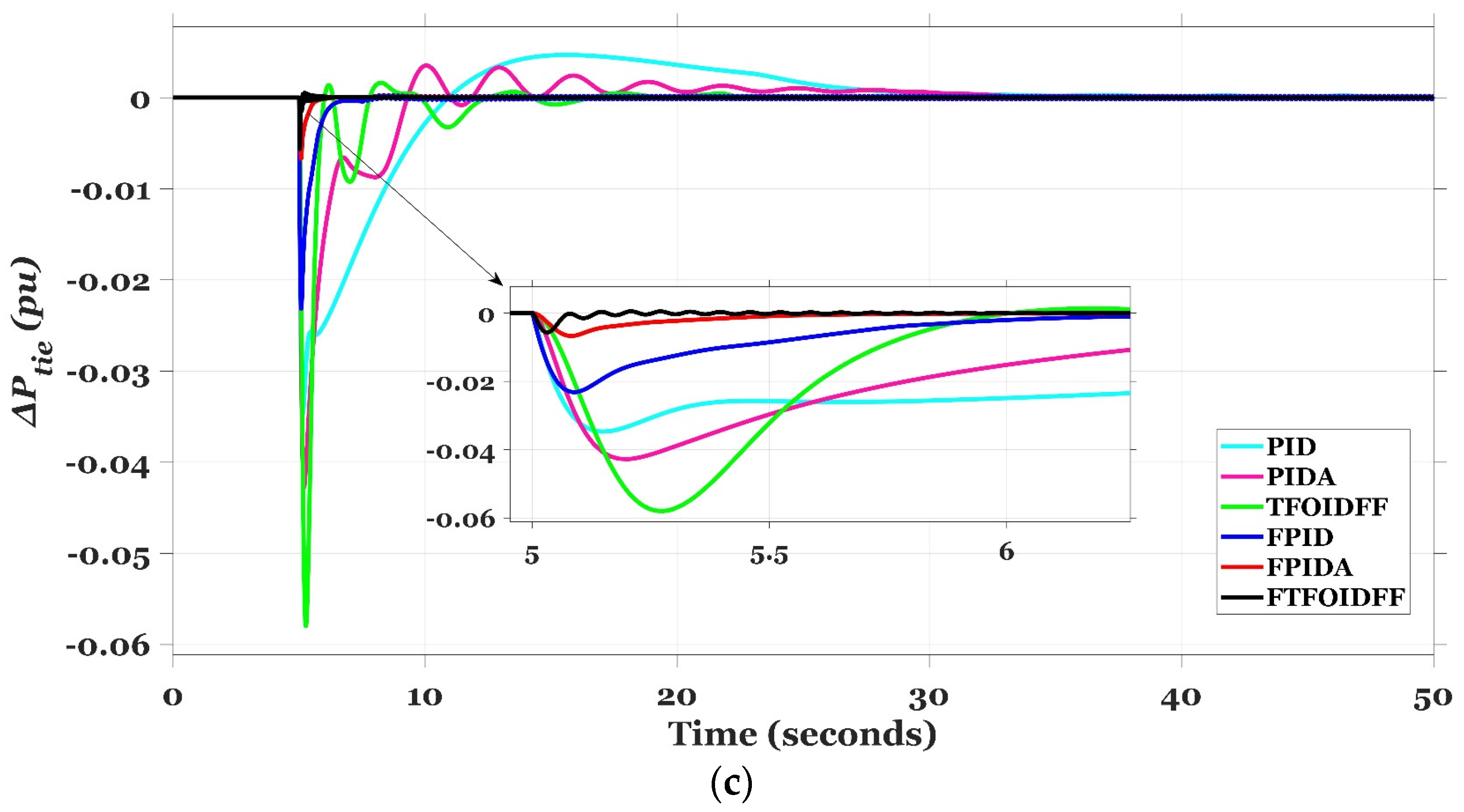
4.1. Case I: 10% Step Load Perturbation (SLP) at t = 5 s in Area (a)

To validate the superiority of the suggested PDO based FTFOIDFF regulator over the other traditional (i.e., PID, PIDA [66], TFOIDFF [65]) and intelligent (i.e., FPID [67] and FPIDA [68]) control techniques, which are also fine-tuned by PDO algorithm, a 10% step load perturbation (SLP) is applied in area (a) at t = 5 s. Table 3 displays the PDO-optimized controller parameters for the chosen case study. The convergence curve in Figure 15 shows that the proposed PDO-based FTFOIDFF outperforms the aforementioned control techniques. Figure 16 depicts the frequency and tie-line power responses (ΔFa, ΔFb, and ΔPtie) of the investigated hybrid electrical grid for both area (a) and area (b). According to research, the suggested PDO-based FTFOIDFF controller has better system stability and damping characteristics with less overshoots, undershoots, and settling times than the other controllers. While producing 0.0067 pu variation in tie-line power and frequency deviations of 0.0158 Hz and 0.008 Hz, respectively, in areas (a) and (b). Table 4 contains a comprehensive comparative study of the examined controllers for several parameters such as settling time (ST), maximum overshoot (MOS), and maximum undershoot (MUS).

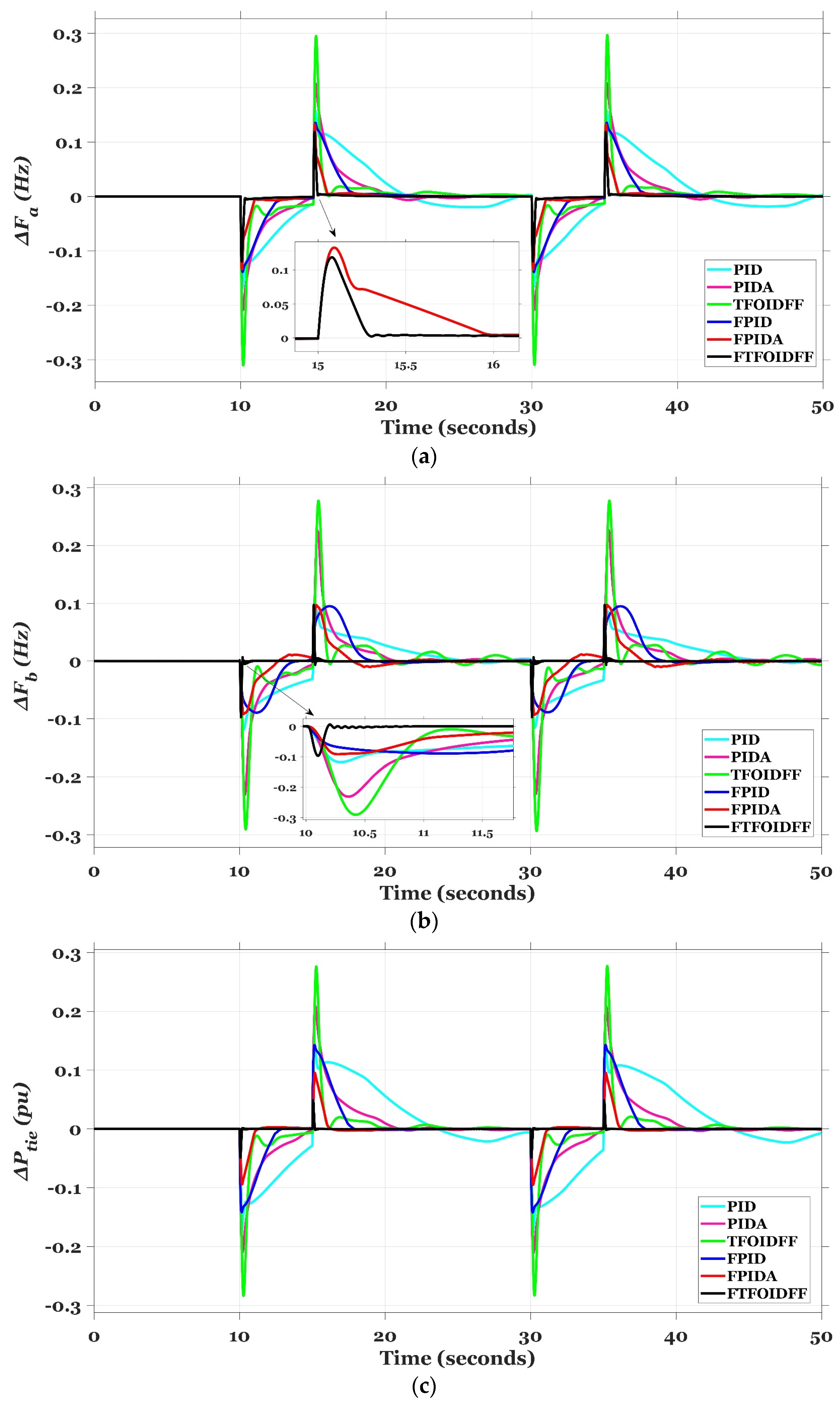
4.2. Case II: Multi-Step Load Perturbation (MSLP) in Area (a)

In this specific case, the ability of the suggested PDO-based FTFOIDFF controller is examined and exposed under the influence of applying a harsh multi-step load change pattern in area (a), where the MSLP is depicted in Figure 17. The MSLP is modelled as a simulation of the series change that occurs in actually connected loads. It is possible to say that the MSLP is thought of as a series-forced switch of generators or a series interrupt of the associated loads. Figure 18 depicts the frequency and power deviation waveforms of the system during the impact of the severe multi-step load fluctuation that the proposed regulator was designed to handle. When compared to the dynamic responses of the other control strategies, the suggested control strategy’s dynamic responses have faster reactions with a small percentage of deviation in their values. The proposed PDO based FTFOIDFF has effectively maintained the entire ITAE value within 4.605, as shown in Table 5, while having low MOS and MUS, as well as a quick and smooth ST. According to Table 5, for instance, and not as a limitation, the proposed controller has been able to acquire a value of the ITAE that is about 37.11 times less than the PID controller, 19.15 times less than the TFOIDFF controller, and 1.34 times lower than the FPIDA controller.

4.3. Case III: Random Load Perturbation (RLP) in Area (b)

After determining the effectiveness of the proposed FTFOIDFF controller in the first two cases, we now proceed to a more challenging scenario in which the severe random load perturbation (RLP), depicted in Figure 19, is applied to area (b) of the power system network under investigation. Practically, the RLP may be thought of as a group of series disturbances that might be represented by connected industrial loads. Figure 20 shows a representation of the system’s reaction to this scenario utilizing a number of different control techniques (specifically, PIDA, TFOIDFF, FPID, FPIDA, and FTFOIDFF controllers that are based on the PDO). The recommended control strategy’s dynamic responses outperform those of the other techniques in terms of speed of response, damping ability, and the values for undershoot, overshoot, and settling time. The system’s dynamic performance, as measured by the ITAE index, is summarized in Table 6. The suggested PDO-based FTFOIDFF has successfully kept the ITAE value within 7.976. This number is around 38.29 times lower than the value asserted by the PID controller, 37.24 times smaller than the value claimed by the PIDA controller, 31.07 times lower than the value asserted by the TFOIDFF controller, 5.57 times lower than the value asserted by the FPID controller, and 3.65 times smaller than the value claimed by the FPIDA controller. This demonstrates that the PDO-based FTFOIDFF controller used for LFC is a stable one.

4.4. Case IV: Pulse Load Perturbation (PLP) in Area (a)

Herein, a severe pulse load perturbation (PLP) with a period of 5 s and high amplitude of 0.5 pu is applied in area (a) twice throughout the simulation duration of 50 s, as shown in Figure 21. Figure 22 presents a visual representation of the area frequencies and tie-line power oscillation reactions that were obtained. When compared with the other control techniques, the results of the simulation reveal that the oscillations are greatly dampened in a short amount of time by the suggested PDO-based FTFOIDFF. Table 7 demonstrates how the suggested controller has the potential to improve the overall performance of the system in terms of the ITAE for each response (i.e., ΔFa, ΔFb, and ΔPtie). According to Table 7, the ITAE index for the ΔFa response is 2.776, the index for Fb is 1.101, and the index for ΔPtie is 0.5113. All of these values are much lower than those of the other controllers that were examined. In addition, as an example and not as a restriction, the proposed controller has been successful in acquiring a value of total ITAE that is about 30.5 times lower than that of the PID controller, 17.7 times lower than that of the PIDA controller, and 13 times lower than that of the FPID controller. This demonstrates the suggested controller’s capability to perform robustly in the face of the high-amplitude PLP.

4.5. Case V: Random Sinusoidal Load Perturbation (RSLP) in Area (a)

Within this case, the analysed system is put through rigorous testing by being subjected to a severe random sinusoidal load perturbation (RSLP) profile in area (a), as seen in Figure 23. The formula that describes the RSLP can be expressed as in Equation (27). Following this, a study of the system’s performance is provided. The proposed FTFOIDFF is tuned using the PDO algorithm, and its efficacy is measured against the objectives of minimising frequency and tie-line power deviations and maintaining system stability, just as was carried out in the earlier scenarios. Table 8 offers an overview of the ITAE values that were generated by a variety of controllers while taking into account the impact of RSLP. Using the recommended FTFOIDFF controller, one may get the lowest feasible ITAE value. The behaviour of the system under these conditions is shown in Figure 24 as well. The oscillation dampening provided by the proposed combination of fuzzy logic and TFOIDFF is clearly better than that of the other tested controllers. As a result, it is clear that the recommended combination was effective in handling the numerous fluctuations and disturbances.
Δ P L = 0.15 sin 2.25 t + 0.24 sin 3.45 t 0.36   s i n ( 4.7 t )

4.6. Case VI: MSLP in Area (a) with 0.01 s Communication Time Delay (CTD)

This case study offers the proposal of the CTD challenge that is applied to the controller output with a time delay value of 0.01 s, and it also takes into consideration the application of the MSLP, used in case II, in order to assess the resilience of the recommended FTFOIDFF regulator in terms of system stabilizing. Figure 25 illustrates the various dynamic reactions of the system, which are represented by ΔFa, ΔFb, and ΔPtie. Figure 25 summarizes and explains the performance of the suggested PDO-based FTFOIDFF controller compared to the other controllers in achieving system stability and reliability after evaluating the influence of time delay in the controller action. The PDO-based FTFOIDFF scheme that was developed exhibits good outcomes when it comes to overcoming all of the problems and achieving better system stability. Table 9 shows the dynamic performance of the system as measured by the ITAE value for ΔFa, ΔFb, and ΔPtie. Table 9 also displays the total ITAE value for the system. For the current case, the proposed PDO-based FTFOIDFF has obtained the lowest fitness function with a value of 6.099. This value is almost 28.09 times lower than the PID controller, 20.51 times lower than the PIDA controller, 14.76 times lower than the TFOIDFF controller, 3.78 times lower than the FPID controller, and 2.09 times lower than the FPIDA controller.

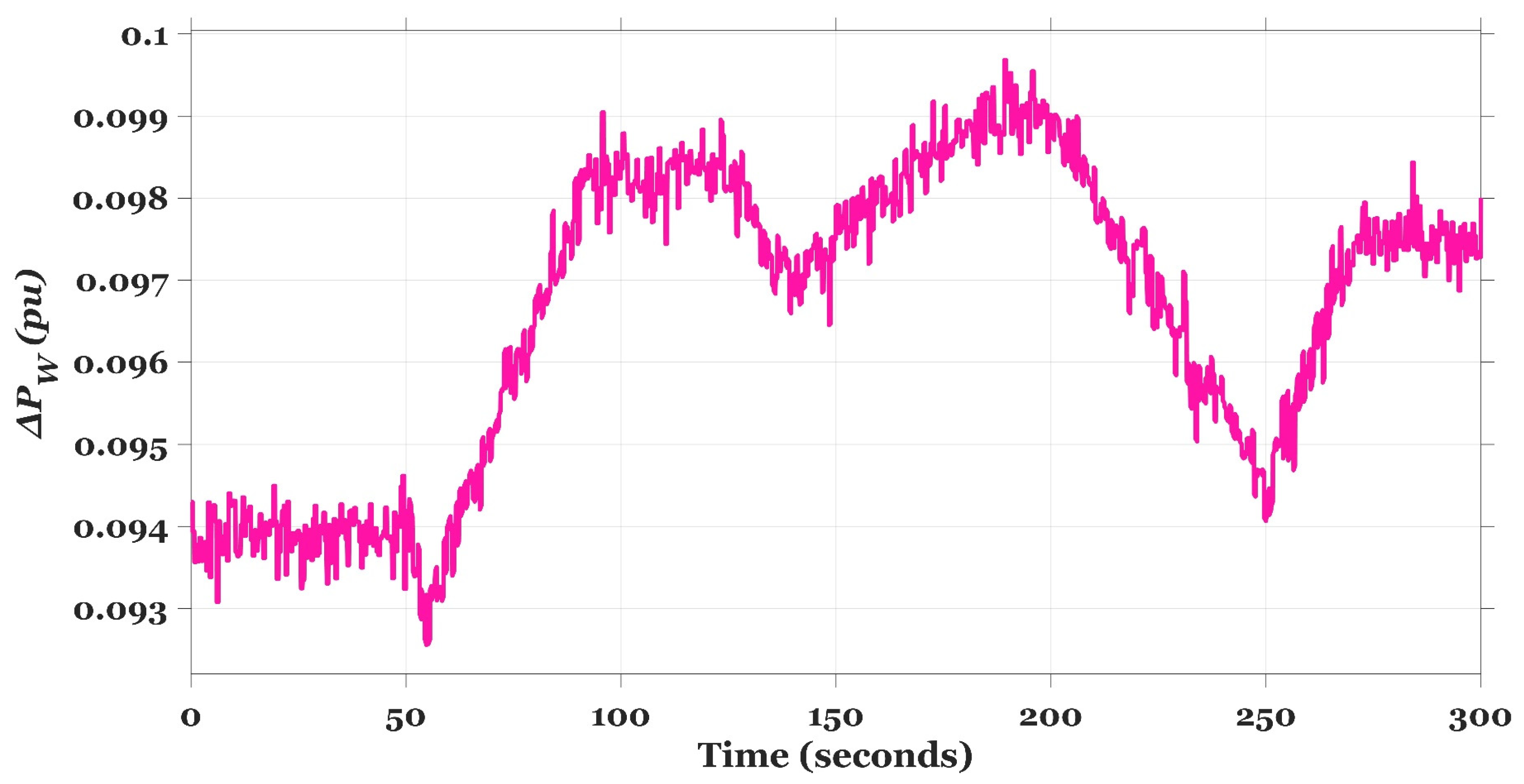
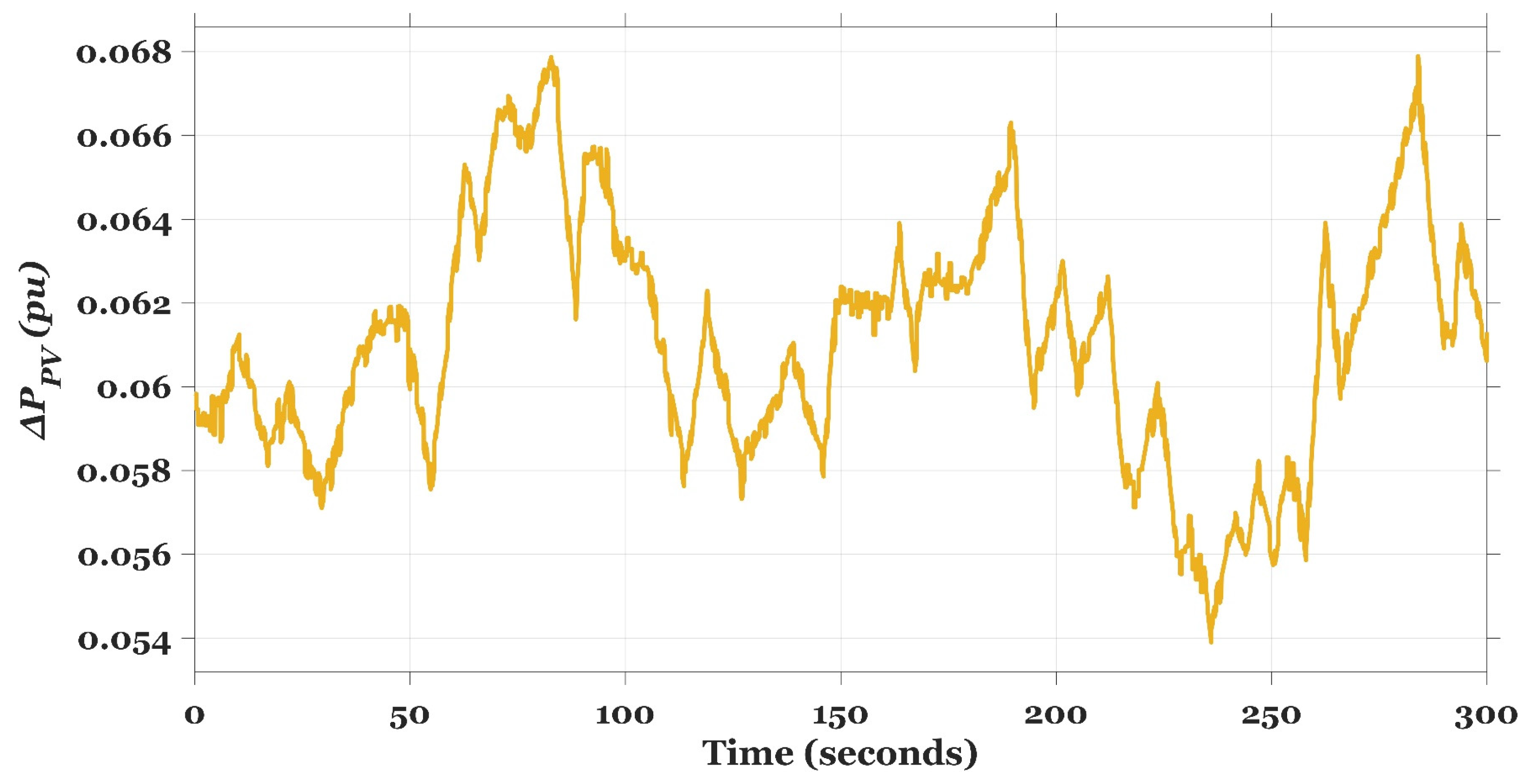
4.7. Case VII: Applying RESs Fluctuations in Both Areas

This study focuses on high RESs penetration (i.e., the integration of a wind farm unit in area (a) and a PV unit in area (b)) to assess the resilience of the proposed PDO-based FTFOIDFF controller in minimizing the examined system fluctuations. The use of RESs places a strain on the hybrid power grid that was investigated due to the drawbacks associated with these sources (i.e., a lack of inertia in the system). The superiority of the suggested FTFOIDFF has been proved and validated via the use of a variety of control techniques, including PID, PIDA, TFOIDFF, FPID, and FPIDA controllers that are based on the PDO. As shown in Figure 26, the integration of RESs causes severe fluctuations in frequency and flow power in the tie-line. Figure 26 illustrates the system dynamics that assure the reliability and efficacy of the proposed PDO based FTFOIDFF controller in dampening variations in frequency and the flow power in the tie-line and boosting the performance of the investigated power grid. These system dynamics are represented in ΔFa, ΔFb, and ΔPtie. The dynamic performance of the power system, as evaluated by the ITAE value, is reported in Table 10. With an index of 5.241, the suggested PDO-based FTFOIDFF has proven to have the best overall fitness performance for this scenario. This number is about 101.14 times less than what the PID controller claims, 60.81 times less than what the PIDA controller claims, 65.81 times less than what the TFOIDFF controller claims, 3.47 times less than what the FPID controller claims, and 1.98 times less than what the FPIDA controller claims.

4.8. Case VIII: Applying RESs Fluctuations with MSLP in Area (b) and RSLP in Area (a)

In this scenario, the impacts of the three scenarios that came before are taken into consideration simultaneously. As a result, the MSLP profile that is described in Figure 17 is put into effect in area (b), and the RSLP profile that is illustrated in Figure 23 is employed in area (a). Furthermore, the RES penetrations are taken into consideration in both areas (i.e., the integration of the wind farm unit in area (a) and the PV unit in area (b)). The purpose of this is to prove that the recommended PDO-based FTFOIDFF is more superior than existing controllers in preserving system stability under stressful circumstances. The outcomes of this case can be seen in Figure 27 and Table 11. It is possible for the presented controller to obtain a value of the fitness function that is nearly 30.1 times less than the value obtained by the PID controller, 17.9 times lesser than the value obtained by the PIDA controller, 10.22 times fewer than the value obtained by the TFOIDFF controller, 6.21 times lesser than the value obtained by the FPID controller, and 1.63 times smaller than the value obtained by the FPIDA controller. Consequently, it is obvious that the suggested FTFOIDFF controller is an outstanding one that succeeds in effectively managing the many variations and disturbances at the same time.

4.9. Case IX: UPFC and SMES Effect on the Studied System with 30% SLP in Area (a)

In this case, the capability of UPFC and SMES, together with the proposed FTFOIDFF, in improving the dynamic performance of the power system was validated by applying 30% SLP in area (a) while testing system performance for the following cases: without UPFC and SMES units, with UPFC only, with SMES only, and with coordinated application of UPFC and SMES. Figure 28 depicts the dynamics of the system, which indicates very clearly that coordinated application of UPFC and SMES leads to a considerable increase in system performance. This improvement may be measured in terms of least undershoot and overshoot in frequency oscillations, as well as tie-line power exchange. Figure 28 makes it abundantly clear that longer settling times and significant overshoots and undershoots are produced by a system that does not have UPFC and SMES. The undershoot frequency decreased to 0.106 Hz and the settling time decreased to 1.28 s after connecting the SMES units in both regions; the settling time was significantly improved from 1.3 s to 0.5 s when UPFC was applied alone; and the undershoot frequency and settling time were further improved to 0.06 Hz and 0.2 s, respectively, when UPFC and SMES were applied in simultaneously. In addition to that, the fitness function, also known as ITAE, has been improved to 0.201. Table 12 summarizes the whole examination of this case.

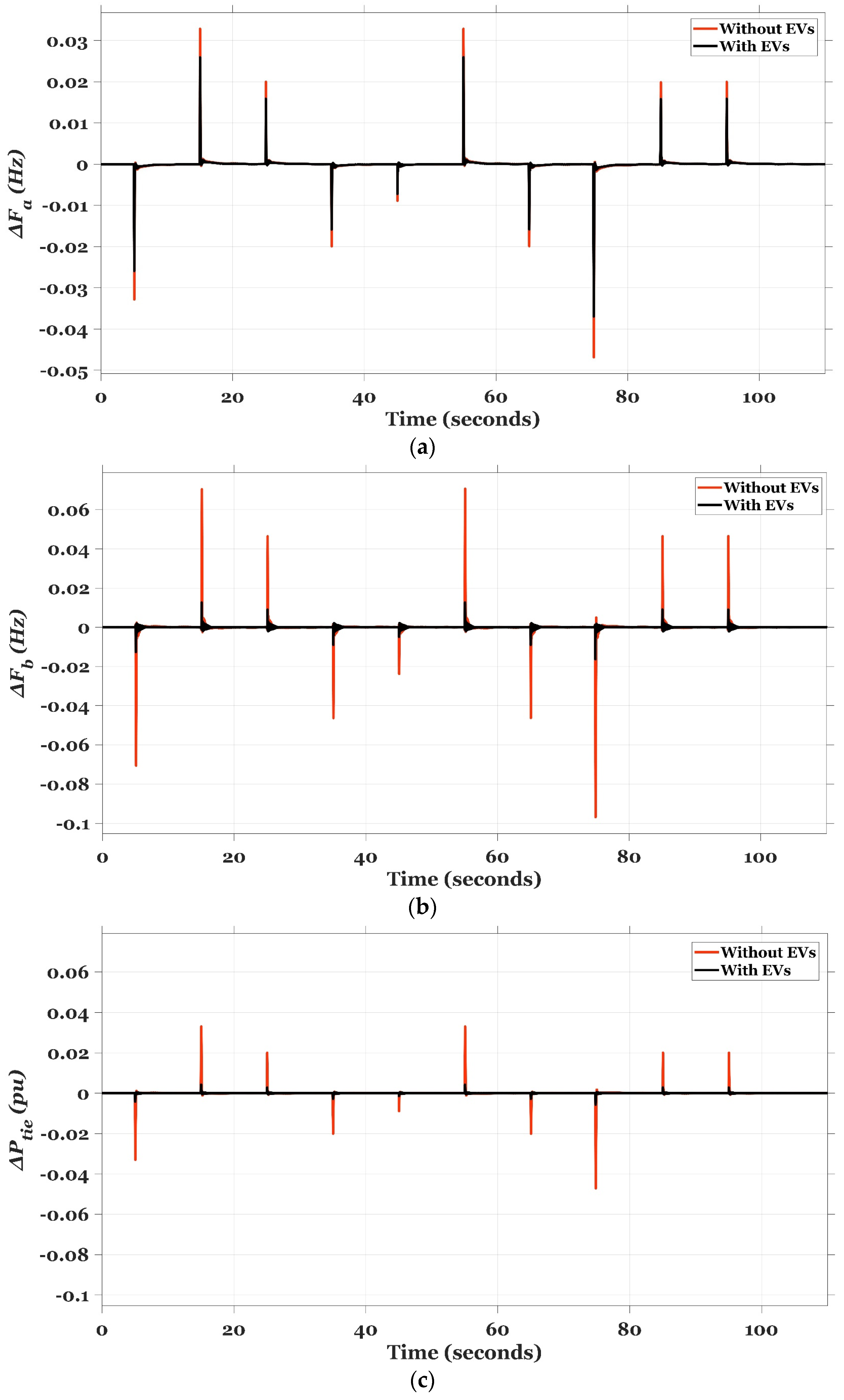
4.10. Case X: EVs Effect on the Studied System with MSLP in Area (a)

This scenario depicts the integration of EVs into both regions of the power grid that was investigated in order to assess the effectiveness of EVs in managing the studied system frequency and the flow of power between the two areas. Figure 29 provides a description of the different dynamic system responses that are expressed by the parameters ΔFa, ΔFb, and ΔPtie. In Table 13, we can see the ITAE values that correspond to the aforementioned variations in system dynamics as a result of changes in both area frequencies and power flow inside the tie line. If electric vehicles (EVs) are incorporated into the system, the overall ITAE of the system’s dynamics falls to 4.605, an improvement of 30.9%. Table 13 demonstrates that the proposed PDO-based FTFOIDFF that takes into account the penetration of EVs in the studied system obtains greater system stability than if these vehicles were not considered. In a nutshell, the incorporation of electric vehicles (EVs) into the power grid that was investigated has the potential to help reduce frequency fluctuations thanks to the energy storage capacity of EVs. This capacity provides the system with additional power under abnormal situations, which helps to ensure that all of the system’s dynamic responses remain within acceptable bounds.

4.11. Case XI: Sensitivity Analysis

Sensitivity refers to a system’s resilience in the face of perturbations to its parameters that fall within a predefined tolerance range. In this part, the resilience of the power system is tested by modifying system parameters such as τ g h , τ c d , y c , B , k E V , and T 12 from their nominal values in the range of + 25 % to 25 % without changing the optimal settings of the proposed FTFOIDFF controller that was provided in case I. The results of the system’s performance are presented in Table 14 for a step load change of 10% in area (a) under both nominal and variable conditions. When the above parameters are changed, it is possible to observe that the dynamic responses of ΔFa, ΔFb, and ΔPtie are barely impacted as a result. In addition, the MOS and MUS scarcely vary at all in comparison to the regular operation, however the settling time is somewhat altered in some instances. On the other hand, the dynamic performance of the suggested system is unaffected by any changes in the other system characteristics. As a consequence of this, the PDO-based FTFOIDFF controller that was presented is reliable and demonstrates a high level of effectiveness in preserving system stability even when system parameters are altered.
In closing, the power system’s network security has steadily become the primary focus of attention as a result of the ongoing growth of the power system communication network and the subsequent expansion of the coverage area. Since the frequency deviation and the tie-line power signals in the LFC system need to be transferred over a long distance, it is conceivable for an attack to be carried out by the insertion of fake data during the process of signal collecting and transmission. By making unauthorized changes to the system’s frequency deviation and tie-line power, the system either incorrectly calculates the value of area control error or compels the load frequency control system to overshoot, which results in frequency oscillation. Moreover, when EVs are integrated into the LFC system, they can be viewed as both the power source and burden for the grid. However, the LFC system that includes EVs is susceptible to covert crimes, and as a result, the power system’s dependable operating performance and security will be compromised. Real-time monitoring and detection methodologies have been established that are very prosperous [75,76]. These methodologies were designed so that these security problems could be solved.

5. Conclusions

This study puts out an innovative method for improving load frequency controllers (LFCs) that makes use of a hybrid approach using fuzzy logic control (FLC) and fractional calculus. This article introduces a maiden controller which is called fuzzy tilted fractional-order integral-derivative with fractional-filter (FTFOIDFF) for use in LFC applications. The proposed FTFOIDFF controller combines the best features of tilt, fuzzy logic, FOPID, and fractional filter regulators. Also, a newly developed metaheuristics optimization method called Prairie Dog Optimizer (PDO) is shown to easily tune the recommended regulator parameters. The model of the system takes into account physical restrictions such the Communication Time Delay (CTD), the reheat turbine, and the Generation Rate Constraint (GRC). The results achieved using PDO are compared to those obtained using SOA, RUN, and CGO algorithms, demonstrating PDO’s superiority. A UPFC is installed in the tie-line, and SMES units are integrated in both areas so as to test their effect on the performance of the system. Furthermore, EVs contributions are included in both areas. The superior efficacy of the proposed FTFOIDFF controller has been demonstrated by comparing its performance to that of a number of conventional (e.g., PID, PIDA, and TFOIDFF) and intelligent (e.g., FPID and FPIDA) regulators from the literature whose parameters are adjusted using PDO algorithm. It has been shown that the recommended FTFOIDFF controller, which is based on the PDO algorithm, works best when subjected to a wide range of load patterns. In addition, the penetration of renewable energy sources and the latency in communication are considered as potential roadblocks to testing the robustness of the proposed controller and achieving greater system stability. To further illustrate the good impact that SMES, UPFC, and EVs units have on the system as a whole, a variety of scenarios have been created. The sensitivity of the system is evaluated by making alterations to the system’s parameters from their baseline values. The simulation results show that, despite the various challenges mentioned above, the proposed FTFOIDFF controller based on the PDO is capable of reaching higher levels of system stability. Furthermore, following research, pros may be summarized as follows:
  • The proposed control structure has efficiently improved frequency stability in a multi-area power system with severe RES penetrations.
  • Integrating the benefits of tilt, fuzzy logic, FOPID, and fractional filter regulators in a single controller known as FTFOIDFF, which has superior performance over the other recent control structures.
  • Application of a nature-inspired metaheuristic optimization technique that was recently developed (i.e., the Prairie Dog Optimizer, or PDO) for the purpose of fine-tuning not only the recommended controller settings but also the MFs of the FLC’s inputs and outputs in an effective manner.
  • Validation of the positive effect of the integration of SMES, UPFC, and EVs in enhancing frequency performance during several harsh disturbances.
Also, cons can be abridged as following:
  • The inclusion of conventional controllers for comparison with intelligent fuzzy-based controllers is unfair, as the incorporation of intelligent controllers, such as fuzzy logic or artificial neural networks, enhances the frequency response performance excessively.
  • The use of simple structured models for EV, SMES, and UPFC will not reveal the full impact of these devices or the uncertainties that may be introduced into the systems as a result of their incorporation.
Finally, for future work, the investigated two-area power system can be expanded to three or four areas, and a more complex model for SMES, UPFC, and EVs can be considered.

Author Contributions

The authors confirm the final authorship for this manuscript. All authors have read and agreed to the published version of the manuscript.

Funding

This research work was funded by Institutional Fund Projects under grant no. (IFPIP: 1428-135-1443). The authors gratefully acknowledge technical and financial support provided by the Ministry of Education and King Abdulaziz University, DSR, Jeddah, Saudi Arabia.

Data Availability Statement

The data is available on request from the authors.

Conflicts of Interest

The authors declare no conflict of interest.

Nomenclature

FLCFuzzy Logic Control
FTFOIDFFFuzzy Tilted Fractional Order Integral Derivative with Fractional Filter
PDOPrairie Dog Optimizer
SOASeagull Optimisation Algorithm
RUNRunge Kutta optimizer
CGOChaos Game Optimizer
LFCLoad Frequency Control
CTDCommunication Time Delay
GRCGeneration Rate Constraint
UPFCUnified Power Flow Controller
SMESSuperconducting Magnetic Energy Storage
EVElectric Vehicle
PIDProportional Integral Derivative
PIDAProportional Integral Derivative Acceleration
SLPStep Load Perturbation
MSLPMulti-Step Load Perturbation
RLPRandom Load Perturbation
RSLPRandom Sinusoidal Load Perturbation
PLPPulse Load Perturbation
AGCAutomatic Generation Control
RESRenewable Energy Sources
PVPhotovoltaic
FACTSFlexible Alternating Current Transmission Systems
FOFractional Order
PCSPower Conversion System
PDPrairie Dog
CTCoterie
LBLower Boundary
UBUpper Boundary
GBGlobal Best
iterCurrent Iteration
MaxiterMaximum Iteration Number
MFsMembership Functions
EError
DOEDerivative of Error
NBNegative Big
NSNegative Small
ZZero
PSPositive Small
PBPositive Big
FISFuzzy Interface System
U 1 First Control Law
U t Total Control Law
G C TFOIDFF Controller’s Transfer Function
t s i m Simulation Time
K t Tilt Gain
K i Integral Gain
K d Derivative Gain
n Tilt Fractional Order Power
λ i Fractional Order Integral Operator
μ d Fractional Order Derivative Operator
λ f Fractional Order Filter Operator
N f Fractional Filter Coefficient
K 1 ,   K 2 Scaling Factor of the FLC inputs
ACEArea Control Error
ITAEIntegral Time Absolute Error
MOSMaximum Overshoot
MUSMaximum Undershoot
STSettling Time
ΔFaThe frequency deviation of Area (a)
ΔFbThe frequency deviation of Area (b)
ΔPtieThe tie-line power deviation

Appendix A. The Nominal Values of the Power System’s Parameters

ParameterNominal ValueParameter Definition
τ s g 0.08 sGovernor time constant
k r 0.3 sGain of reheater steam turbine
τ r 10.2 sThe time constant of reheater steam turbine
τ t 0.3 sSteam turbine time constant
τ g h 0.2 sHydroelectric turbine speed governor time constant
τ r s 4.9 sHydro turbine speed governor reset time
τ r h 28.749 sTime constant of the transient droop
τ w 1.1 sAverage water string time in penstock
b g 0.049 sGas turbine constant of valve positioner
c g 1Valves’ gas turbine positioner constant
x c 0.6 sGas turbine governor’s lead time constant
y c 1.1 sGas turbine governor’s lag time constant
τ c r 0.01 sCombustion response time delay in a gas turbine
τ f c 0.239 sGas turbine fuel time constant
τ c d 0.2 sVolume-time constant for gas turbine compressor discharge
k p s 1 , k p s 2 68.965, 68.965Power system gains
τ p s 1 , τ p s 2 11.49, 11.49 sPower system time constants
T 12 0.0433 MWCoefficient of synchronizing
k S M E S ( a ) , k S M E S ( b ) 1, 1Gains of SMES
τ S M E S ( a ) , τ S M E S ( b ) 0.07 sTime constants of SMES units
τ U P F C 0.003 sTime constant of UPFC unit
k E V ( a ) , k E V ( b ) 1Gains of EVs
τ E V ( a ) , τ E V ( b ) 0.28 sTime constants of EVs
B a ,   B b 0.431, 0.431 MW/HzFrequency bias coefficients
R 2.4 Hz/MWGovernor speed regulation constant for thermal, hydro, and gas units
C F T ,   C F H , C F G 0.5435, 0.3261, 0.1304Contribution factors of thermal, hydro, and gas units
GRC with Hydro--------(0.045 pu.MW/s) and (0.06 pu.MW/s. For both rising and decreasing rates), respectively
GRC with Thermal--------The GRC (generation rate constraint) for the thermal unit is set (0.0017 pu.MW/s) For rising and decreasing rates

References

  1. Elgerd, O.I. Electric Energy Systems Theory—An Introduction; Tata McGraw Hill: New Delhi, India, 2000. [Google Scholar]
  2. Kundur, P.S.; Malik, O. Power System Stability and Control, 2nd ed.; McGraw-Hill Education: Columbus, OH, USA, 2022. [Google Scholar]
  3. Bevrani, H. Robust Power System Frequency Control; Springer International Publishing: Cham, Switzerland, 2016. [Google Scholar]
  4. Parmar, K.P.S.; Majhi, S.; Kothari, D.P. Load frequency control of a realistic power system with multi-source power generation. Int. J. Electr. Power Energ. Syst. 2012, 42, 426–433. [Google Scholar] [CrossRef]
  5. Mohanty, B.; Panda, S.; Hota, P.K. Controller parameters tuning of differential evolution algorithm and its application to load frequency control of multi-source power system. Int. J. Electr. Power Energ. Syst. 2014, 54, 77–85. [Google Scholar] [CrossRef]
  6. Yildirim, B.; Gheisarnejad, M.; Khooban, M.H. A robust non-integer controller design for load frequency control in modern marine power grids. IEEE Trans. Emerg. Top. Comput. Intell. 2022, 6, 852–866. [Google Scholar] [CrossRef]
  7. Ahmed, E.M.; Mohamed, E.A.; Elmelegi, A.; Aly, M.; Elbaksawi, O. Optimum Modified Fractional Order Controller for Future Electric Vehicles and Renewable Energy-Based Interconnected Power Systems. IEEE Access 2021, 9, 29993–30010. [Google Scholar] [CrossRef]
  8. Sun, P.; Yun, T.; Chen, Z. Multi-objective robust optimization of multi-energy microgrid with waste treatment. Renew. Energy 2021, 178, 1198–1210. [Google Scholar] [CrossRef]
  9. Xiao, D.; Chen, H.; Wei, C.; Bai, X. Statistical Measure for Risk-seeking Stochastic Wind Power Offering Strategies in Electricity Markets. J. Mod. Power Syst. Clean Energy 2022, 10, 1437–1442. [Google Scholar] [CrossRef]
  10. Said, S.M.; Aly, M.; Hartmann, B.; Mohamed, E.A. Coordinated fuzzy logic-based virtual inertia controller and frequency relay scheme for reliable operation of low-inertia power system. IET Renew. Power Gener. 2021, 15, 1286–1300. [Google Scholar] [CrossRef]
  11. Liu, L.; Hu, Z.; Mujeeb, A. Automatic generation control considering uncertainties of the key parameters in the frequency response model. IEEE Trans. Power Syst. 2022, 37, 4605–4617. [Google Scholar] [CrossRef]
  12. Magdy, G.; Ali, H.; Xu, D. Effective Control of Smart Hybrid Power Systems: Cooperation of Robust LFC and Virtual Inertia Control Systems. CSEE J. Power Energy Syst. 2022, 8, 1583–1593. [Google Scholar] [CrossRef]
  13. Tripathy, S.C.; Kalantar, M.; Balasubramanian, R. Dynamics and stability of wind and diesel turbine generators with superconducting magnetic energy storage unit on an isolated power system. IEEE Trans. Energy Conv. 1991, 6, 579–585. [Google Scholar] [CrossRef]
  14. Abraham, R.J.; Das, D.; Patra, A. Automatic generation control of an interconnected hydrothermal power system considering superconducting magnetic energy storage. Int. J. Electr. Power Energ. Syst. 2007, 29, 571–579. [Google Scholar] [CrossRef]
  15. Banerjee, S.; Chatterjee, J.K.; Tripathy, S.C. Application of magnetic energy storage unit as load-frequency stabilizer. IEEE Trans. Energy Conv. 1990, 5, 46–51. [Google Scholar] [CrossRef]
  16. Abraham, R.J.; Das, D.; Patra, A. AGC of a hydrothermal system with SMES unit. In Proceedings of the 2006 IEEE GCC Conference (GCC), Manama, Bahrain, 20–22 March 2006; pp. 1–7. [Google Scholar]
  17. Padhan, S.; Sahu, R.K.; Panda, S. Automatic generation control with thyristor controlled series compensator including superconducting magnetic energy storage units. Ain Shams Eng. J. 2014, 5, 759–774. [Google Scholar] [CrossRef]
  18. Sudha, K.R.; Vijaya, S.R. Load frequency control of an interconnected reheat thermal system using type-2 fuzzy system including SMES units. Int. J. Electr. Power Energ. Syst. 2012, 43, 1383–1392. [Google Scholar] [CrossRef]
  19. Hingorani, N.G.; Gyugyi, L. Understanding FACTS: Concepts and Technology of Flexible AC Transmission System; IEEE Press: New York, NY, USA, 2000. [Google Scholar]
  20. Praghnesh, B.; Ranjit, R. Load frequency stabilization by coordinated control of Thyristor Controlled Phase Shifters and superconducting magnetic energy storage for three types of interconnected two-area power systems. Int. J. Electr. Power Energ. Syst. 2010, 32, 1111–1124. [Google Scholar]
  21. Praghnesh, B.; Ranjit, R. Comparative performance evaluation of SMES-SMES, TCPS-SMES and SSSC-SMES controllers in automatic generation control for a two-area hydro-hydro system. Int. J. Electr. Power Energ. Syst. 2011, 32, 1585–1597. [Google Scholar]
  22. Paliwal, N.; Srivastava, L.; Pandit, M. Application of grey wolf optimization algorithm for load frequency control in multi-source single area power system. Evol. Intell. 2022, 15, 563–584. [Google Scholar] [CrossRef]
  23. Aryan, P.; Ranjan, M.; Shankar, R. Deregulated LFC scheme using equilibrium optimized Type-2 fuzzy controller. WEENTECH Proc. Energy 2021, 8, 494–505. [Google Scholar] [CrossRef]
  24. Dreidy, M.; Mokhlis, H.; Mekhilef, S. Inertia response and frequency control techniques for renewable energy sources: A review. Renew. Sustain. Energy Rev. 2017, 69, 144–155. [Google Scholar] [CrossRef]
  25. Fernández-Guillamón, A.; Gómez-Lázaro, E.; Muljadi, E.; Molina-García, Á. Power systems with high renewable energy sources: A review of inertia and frequency control strategies over time. Renew. Sustain. Energy Rev. 2019, 115, 109369. [Google Scholar] [CrossRef]
  26. Singh, V.P.; Kishor, N.; Samuel, P. Improved load frequency control of power system using LMI based PID approach. J. Franklin Inst. 2017, 354, 6805–6830. [Google Scholar] [CrossRef]
  27. Jagatheesan, K.; Anand, B.; Samanta, S.; Dey, N.; Ashour, A.S.; Balas, V.E. Particle swarm optimisation-based parameters optimisation of PID controller for load frequency control of multi-area reheat thermal power systems. Int. J. Adv. Intell. Paradig. 2017, 9, 464. [Google Scholar] [CrossRef]
  28. Hasanien, H.M. Whale optimisation algorithm for automatic generation control of interconnected modern power systems including renewable energy sources. IET Gener. Transm. Distrib. 2018, 12, 607–614. [Google Scholar] [CrossRef]
  29. Mehta, P.; Bhatt, P.; Pandya, V. Optimized coordinated control of frequency and voltage for distributed generating system using Cuckoo Search Algorithm. Ain Shams Eng. J. 2018, 9, 1855–1864. [Google Scholar] [CrossRef]
  30. Sobhy, M.A.; Abdelaziz, A.Y.; Hasanien, H.M.; Ezzat, M. Marine predators algorithm for load frequency control of modern interconnected power systems including renewable energy sources and energy storage units. Ain Shams Eng. J. 2021, 12, 3843–3857. [Google Scholar] [CrossRef]
  31. Nayak, S.R.; Khadanga, R.K.; Arya, Y.; Panda, S.; Sahu, P.R. Influence of ultra-capacitor on AGC of five-area hybrid power system with multi-type generations utilizing sine cosine adopted dingo optimization algorithm. Electr. Power Syst. Res. 2023, 223, 109513. [Google Scholar] [CrossRef]
  32. Veerendar, T.; Kumar, D.; Sreeram, V. Maiden application of colliding bodies optimizer for load frequency control of two-area nonreheated thermal and hydrothermal power systems. Asian J. Control. 2023, 25, 3443–3455. [Google Scholar] [CrossRef]
  33. Murugesan, D.; Jagatheesan, K.; Shah, P.; Sekhar, R. Fractional order PIλDμ controller for microgrid power system using cohort intelligence optimization. Results Control. Optim. 2023, 11, 100218. [Google Scholar] [CrossRef]
  34. Andic, C.; Ozumcan, S.; Varan, M.; Ozturk, A. A novel Sea Horse Optimizer based load frequency controller for two-area power system with PV and thermal units. Preprints 2023, 2023040368. [Google Scholar] [CrossRef]
  35. Gheisarnejad, M. An effective hybrid harmony search and cuckoo optimization algorithm based fuzzy PID controller for load frequency control. Appl. Soft Comput. 2018, 65, 121–138. [Google Scholar] [CrossRef]
  36. Ahmed, M.; Magdy, G.; Khamies, M.; Kamel, S. Modified TID controller for load frequency control of a two-area interconnected diverse-unit power system. Int. J. Electr. Power Energy Syst. 2022, 135, 107528. [Google Scholar] [CrossRef]
  37. Zahariev, A.; Kiskinov, H. Asymptotic Stability of the Solutions of Neutral Linear Fractional System with Nonlinear Perturbation. Mathematics 2020, 8, 390. [Google Scholar] [CrossRef]
  38. Milev, M.; Zlatev, S. A Note about Stability of Fractional Retarded Linear Systems with Distributed Delays. Int. J. Pure Appl. Math. 2017, 115, 873–881. [Google Scholar] [CrossRef]
  39. Kiskinov, H.; Milev, M.; Zahariev, A. About the Resolvent Kernel of Neutral Linear Fractional System with Distributed Delays. Mathematics 2022, 10, 4573. [Google Scholar] [CrossRef]
  40. Kumar Sahu, R.; Panda, S.; Biswal, A.; Chandra Sekhar, G.T. Design and analysis of tilt integral derivative controller with filter for load frequency control of multi-area interconnected power systems. ISA Trans. 2016, 61, 251–264. [Google Scholar] [CrossRef] [PubMed]
  41. Topno, P.N.; Chanana, S. Load frequency control of a two-area multi-source power system using a tilt integral derivative controller. J. Vib. Control 2018, 24, 110–125. [Google Scholar] [CrossRef]
  42. Shouran, M.; Anayi, F.; Packianather, M.; Habil, M. Load frequency control based on the Bees Algorithm for the Great Britain power system. Designs 2021, 5, 50. [Google Scholar] [CrossRef]
  43. Bayati, N.; Dadkhah, A.; Vahidi, B.; Sadeghi, S.H.H. Fopid design for load-frequency control using genetic algorithm. Sci. Int. 2015, 27, 3089–3094. [Google Scholar]
  44. Pan, I.; Das, S. Fractional order AGC for distributed energy resources using robust optimization. IEEE Trans. Smart Grid 2016, 7, 2175–2186. [Google Scholar] [CrossRef]
  45. Ramachandran, R.; Satheesh Kumar, J.; Madasamy, B.; Veerasamy, V. A hybrid MFO-GHNN tuned self-adaptive FOPID controller for ALFC of renewable energy integrated hybrid power system. IET Renew. Power Gener. 2021, 15, 1582–1595. [Google Scholar] [CrossRef]
  46. Sambariya, D.K.; Nagar, O.; Sharma, A.K. Application of FOPID design for LFC using flower pollination algorithm for three-area power system. Univers. J. Contr. Autom. 2020, 8, 212695735. [Google Scholar] [CrossRef]
  47. Alharbi, M.; Ragab, M.; AboRas, K.M.; Kotb, H.; Dashtdar, M.; Shouran, M.; Elgamli, E. Innovative AVR-LFC design for a multi-area power system using hybrid fractional-order PI and PIDD2 controllers based on dandelion optimizer. Mathematics 2023, 11, 1387. [Google Scholar] [CrossRef]
  48. Latif, A.; Hussain, S.M.S.; Das, D.C.; Ustun, T.S. Optimum synthesis of a BOA optimized novel dual-stage PI-(1+ID) controller for frequency response of a microgrid. Energies 2020, 13, 3446. [Google Scholar] [CrossRef]
  49. Mohamed, E.A.; Ahmed, E.M.; Elmelegi, A.; Aly, M.; Elbaksawi, O.; Mohamed, A.-A.A. An optimized hybrid fractional order controller for frequency regulation in multi-area power systems. IEEE Access 2020, 8, 213899–213915. [Google Scholar] [CrossRef]
  50. Yogendra, A. A novel CFFOPI-FOPID controller for AGC performance enhancement of single and multi-area electric power systems. ISA Trans. 2020, 100, 126–135. [Google Scholar] [CrossRef]
  51. Yogendra, A. A new optimized fuzzy FOPI-FOPD controller for automatic generation control of electric power systems. J. Franklin Inst. 2019, 356, 5611–5629. [Google Scholar] [CrossRef]
  52. Gheisarnejad, M.; Khooban, M.H. Design an optimal fuzzy fractional proportional integral derivative controller with derivative filter for load frequency control in power systems. Trans. Inst. Meas. Control 2019, 41, 2563–2581. [Google Scholar] [CrossRef]
  53. Yogendra, A. Improvement in automatic generation control of two-area electric power systems via a new fuzzy aided optimal PIDN-FOI controller. ISA Trans. 2018, 80, 475–490. [Google Scholar] [CrossRef]
  54. Arya, Y.; Kumar, N.; Dahiya, P.; Sharma, G.; Çelik, E.; Dhundhara, S.; Sharma, M. Cascade-I λ D μ N controller design for AGC of thermal and hydro-thermal power systems integrated with renewable energy sources. IET Renew. Power Gener. 2021, 15, 504–520. [Google Scholar] [CrossRef]
  55. Magdy, G.; Shabib, G.; Elbaset, A.A.; Mitani, Y. Frequency stabilization of renewable power systems based on MPC with application to the Egyptian grid. IFAC-PapersOnLine 2018, 51, 280–285. [Google Scholar] [CrossRef]
  56. Zhang, C.; Wang, S.; Zhao, Q. Distributed economic MPC for LFC of multi-area power system with wind power plants in power market environment. Int. J. Electr. Power Energy Syst. 2020, 126, 106548. [Google Scholar] [CrossRef]
  57. Fathy, A.; Kassem, A.M. Antlion optimizer-ANFIS load frequency control for multi-interconnected plants comprising photovoltaic and wind turbine. ISA Trans. 2018, 87, 282–296. [Google Scholar] [CrossRef]
  58. Patowary, M.; Panda, G.; Naidu, B.R.; Deka, B.C. ANN-based adaptive current controller for on-grid DG system to meet frequency deviation and transient load challenges with hardware implementation. IET Renew. Power Gener. 2017, 12, 61–71. [Google Scholar] [CrossRef]
  59. Dombi, J.; Hussain, A. A new approach to fuzzy control using the distending function. J. Process. Control. 2019, 86, 16–29. [Google Scholar] [CrossRef]
  60. Valdez, F.; Castillo, O.; Peraza, C. Fuzzy logic in dynamic parameter adaptation of Harmony search optimization for benchmark functions and fuzzy controllers. Int. J. Fuzzy Syst. 2020, 22, 1198–1211. [Google Scholar] [CrossRef]
  61. Yakout, A.H.; Kotb, H.; Hasanien, H.M.; Aboras, K.M. Optimal fuzzy PIDF load frequency controller for hybrid microgrid system using marine predator algorithm. IEEE Access 2021, 9, 54220–54232. [Google Scholar] [CrossRef]
  62. Rajesh, K.S.; Dash, S.S. Load frequency control of autonomous power system using adaptive fuzzy based PID controller optimized on improved sine cosine algorithm. J. Ambient. Intell. Humaniz. Comput. 2018, 10, 2361–2373. [Google Scholar] [CrossRef]
  63. Mishra, D.; Sahu, P.C.; Prusty, R.C.; Panda, S. Fuzzy adaptive Fractional Order-PID controller for frequency control of an Islanded Microgrid under stochastic wind/solar uncertainties. Int. J. Ambient. Energy 2021, 43, 4602–4611. [Google Scholar] [CrossRef]
  64. Osinski, C.; Leandro, G.V.; Oliveira, G.H.d.C. A new hybrid load frequency control strategy combining fuzzy sets and differential evolution. J. Control. Autom. Electr. Syst. 2021, 32, 1627–1638. [Google Scholar] [CrossRef]
  65. Mohamed, E.A.; Aly, M.; Watanabe, M. New tilt fractional-order integral derivative with fractional filter (TFOIDFF) controller with artificial hummingbird optimizer for LFC in renewable energy power grids. Mathematics 2022, 10, 3006. [Google Scholar] [CrossRef]
  66. Yakout, A.H.; Attia, M.A.; Kotb, H. Marine predator algorithm based cascaded PIDA load frequency controller for electric power systems with wave energy conversion systems. Alex. Eng. J. 2021, 60, 4213–4222. [Google Scholar] [CrossRef]
  67. Pradhan, P.C.; Sahu, R.K.; Panda, S. Firefly algorithm optimized fuzzy PID controller for AGC of multi-area multi-source power systems with UPFC and SMES. Eng. Sci. Technol. Int. J. 2016, 19, 338–354. [Google Scholar] [CrossRef]
  68. AboRas, K.M.; Ragab, M.; Shouran, M.; Alghamdi, S.; Kotb, H. Voltage and frequency regulation in smart grids via a unique Fuzzy PIDD2 controller optimized by Gradient-Based Optimization algorithm. Energy Rep. 2023, 9, 1201–1235. [Google Scholar] [CrossRef]
  69. Elkasem, A.H.A.; Khamies, M.; Hassan, M.H.; Agwa, A.M.; Kamel, S. Optimal design of TD-TI controller for LFC considering renewables penetration by an improved chaos game optimizer. Fractal Fract. 2022, 6, 220. [Google Scholar] [CrossRef]
  70. Gyugyi, L. Unified power-flow control concept for flexible AC transmission systems. IEE Proc. 1992, 139, 323. [Google Scholar] [CrossRef]
  71. Khadanga, R.K.; Panda, S. Gravitational search algorithm for Unified Power Flow Controller based damping controller design. In Proceedings of the 2011 International Conference on Energy, Automation and Signal, Bhubaneswar, India, 28–30 December 2011. [Google Scholar]
  72. Kazemi, A.; Shadmesgaran, M.R. Extended supplementary Controller of UPFC to improve damping inter-area oscillations considering inertia coefficient. Int. J. Energy 2008, 2, 25–36. [Google Scholar]
  73. Ezugwu, A.E.; Agushaka, J.O.; Abualigah, L.; Mirjalili, S.; Gandomi, A.H. Prairie dog optimization algorithm. Neural Comput. Appl. 2022, 34, 20017–20065. [Google Scholar] [CrossRef]
  74. Yang, X.-S.; Deb, S. Cuckoo search via Lévy flights. In Proceedings of the 2009 World Congress on Nature & Biologically Inspired Computing (NaBIC), Coimbatore, India, 9–11 December 2009; pp. 210–214. [Google Scholar]
  75. Zhu, R.; Huang, C.; Deng, S.; Li, Y. Detection of false data injection attacks based on Kalman filter and controller design in power system LFC. J. Phys. Conf. Ser. 2021, 1861, 012120. [Google Scholar] [CrossRef]
  76. Wu, Z.; Tian, E.; Chen, H. Covert attack detection for LFC systems of electric vehicles: A dual time-varying coding method. IEEE ASME Trans. Mechatron. 2023, 28, 681–691. [Google Scholar] [CrossRef]
Figure 1. The schematic diagram of investigated power grid.
Fractalfract 07 00807 g001
Figure 2. The examined power grid in form of transfer function model.
Fractalfract 07 00807 g002
Figure 3. UPFC integration in a dual area linked power system [67].
Fractalfract 07 00807 g003
Figure 4. The circuit diagram representation of SMES [67].
Fractalfract 07 00807 g004
Figure 5. The wind system representation in MATLAB/Simulink program (R2022b) [69].
Fractalfract 07 00807 g005
Figure 6. The wind model generated power.
Fractalfract 07 00807 g006
Figure 7. The PV system representation in MATLAB/Simulink program (R2022b) [69].
Fractalfract 07 00807 g007
Figure 8. The PV model generated power.
Fractalfract 07 00807 g008
Figure 9. The EV system representation in MATLAB/Simulink program (R2022b).
Fractalfract 07 00807 g009
Figure 10. PDO algorithm’s flow chart representation.
Fractalfract 07 00807 g010
Figure 11. The configuration of TFOIDFF controller [65].
Fractalfract 07 00807 g011
Figure 12. The configuration of the FTFOIDFF controller.
Fractalfract 07 00807 g012
Figure 13. The MFs of the proposed FTFOIDFF for both areas. (a) MFs of the controllers in area 1; (b) MFs of the controllers in area 2.
Fractalfract 07 00807 g013
Figure 14. The convergence curve characteristics of SOA, RUN, CGO, and PDO.
Fractalfract 07 00807 g014
Figure 15. The convergence curve characteristics of the compared controllers.
Fractalfract 07 00807 g015
Figure 16. The system dynamics for Case I. (a) ΔFa; (b) ΔFb; (c) ΔPtie.
Fractalfract 07 00807 g016aFractalfract 07 00807 g016b
Figure 17. MSLP profile.
Fractalfract 07 00807 g017
Figure 18. The system dynamics for Case II. (a) ΔFa; (b) ΔFb; (c) ΔPtie.
Fractalfract 07 00807 g018
Figure 19. The RLP profile.
Fractalfract 07 00807 g019
Figure 20. The system dynamics for Case III. (a) ΔFa; (b) ΔFb; (c) ΔPtie.
Fractalfract 07 00807 g020
Figure 21. The PLP profile.
Fractalfract 07 00807 g021
Figure 22. The system dynamics for Case IV. (a) ΔFa; (b) ΔFb; (c) ΔPtie.
Fractalfract 07 00807 g022
Figure 23. The RSLP profile.
Fractalfract 07 00807 g023
Figure 24. The system dynamics for Case V. (a) ΔFa; (b) ΔFb; (c) ΔPtie.
Fractalfract 07 00807 g024
Figure 25. The system dynamics for Case VI. (a) ΔFa; (b) ΔFb; (c) ΔPtie.
Fractalfract 07 00807 g025aFractalfract 07 00807 g025b
Figure 26. The system dynamics for Case VII. (a) ΔFa; (b) ΔFb; (c) ΔPtie.
Fractalfract 07 00807 g026aFractalfract 07 00807 g026b
Figure 27. The system dynamics for Case VIII. (a) ΔFa; (b) ΔFb; (c) ΔPtie.
Fractalfract 07 00807 g027
Figure 28. The system dynamics for Case IX. (a) ΔFa; (b) ΔFb; (c) ΔPtie.
Fractalfract 07 00807 g028aFractalfract 07 00807 g028b
Figure 29. The system dynamics for Case X. (a) ΔFa; (b) ΔFb; (c) ΔPtie.
Fractalfract 07 00807 g029
Table 1. The examined power grid’s transfer functions [69].
Power PlanetModelTransfer Function
ThermalGovernor 1 τ s g s + 1
Reheat k r τ r   s + 1 τ r s + 1
Turbine 1 τ t s + 1
HydraulicGovernor 1 τ g h s + 1
Transient droop compensation τ r s s + 1 τ r h s + 1
turbine τ w s + 1 0.5 τ w s + 1
GasValve positioner 1 b g s + c g
Speed governor x c s + 1 y c s + 1
Fuel system and combustor τ c r s + 1 τ f c s + 1
Compressor discharge 1 τ c d s + 1
OthersPower system (a) k p s 1 τ p s 1 s + 1
Power system (b) k p s 2 τ p s 2 s + 1
T-line 2 π T 12 s
SMES (a) k S M E S ( a ) τ S M E S ( a ) s + 1
SMES (b) k S M E S ( b ) τ S M E S ( b ) s + 1
UPFC 1 τ U P F C s + 1
EV (a) k E V ( a ) τ E V ( a ) s + 1
EV (b) k E V ( b ) τ E V ( b ) s + 1
Table 2. FLC rule base.
EDOE
NBSNZSPLP
NBNBNBNSNSZ
NSNBNSNSZPS
ZNSNSZPSPS
PSNSZPSPSPB
PBZPSPSPBPB
Table 3. The optimum parameters of the different controllers.
ControllerThermalHydroGas
PIDArea (a) K p = 0.024 ,   K i = 0.486 ,
K d = 0.293 ,   N f = 102
Area (a) K p = 0.025 ,   K i = 3.573 ,
K d = 2.025 ,   N f = 151
Area (a) K p = 4.993 ,   K i = 4.992 ,
K d = 4.104 ,   N f = 192
Area (b) K p = 0.002 ,   K i = 0.011 ,
K d = 0.218 ,   N f = 290
Area (b) K p = 0.368 ,   K i = 0.176 ,
K d = 0.133 ,   N f = 218
Area (b) K p = 0.521 ,   K i = 1.209 ,
K d = 4.804 ,   N f = 146
PIDAArea (a) K p = 3.365 ,   K i = 0.775 ,
K d 1 = 1.666 ,   K d 2 = 0.001 ,
N f 1 = 265 ,   N f 2 = 174
Area (a) K p = 0.245 ,   K i = 0.654 ,
K d 1 = 9.895 ,   K d 2 = 0.008 ,
N f 1 = 245 ,   N f 2 = 194
Area (a) K p = 9.996 ,   K i = 9.999 ,
K d 1 = 0.607 ,   K d 2 = 0.031 ,
N f 1 = 191 ,   N f 2 = 345
Area (b) K p = 6.599 ,   K i = 0.487 ,
K d 1 = 1.309 ,   K d 2 = 0.001 ,
N f 1 = 249 ,   N f 2 = 179
Area (b) K p = 0.714 ,   K i = 0.451 ,
K d 1 = 0.217 ,   K d 2 = 0.005 ,
N f 1 = 214 ,   N f 2 = 201
Area (b) K p = 5.969 ,   K i = 0.207 ,
K d 1 = 9.246 ,   K d 2 = 0.003 ,
N f 1 = 164 ,   N f 2 = 312
TFOIDFFArea (a) K t = 11.173 ,   K i = 0.011 ,
K d = 0.024 ,   n = 5.077 ,
λ i = 0.16 ,   μ d = 0.063 ,
λ f = 0.011 ,   N f = 166
Area (a) K t = 0 ,   K i = 4.453 ,
K d = 9.991 ,   n = 2.127 ,
λ i = 1 ,   μ d = 0.922 ,
λ f = 0.015 ,   N f = 177
Area (a) K t = 19.988 ,   K i = 6.801 ,
K d = 0.091 ,   n = 1.5 ,
λ i = 0.004 ,   μ d = 0.074 ,
λ f = 0.694 ,   N f = 113
Area (b) K t = 0.408 ,   K i = 0 ,
K d = 8.042 ,   n = 5.75 ,
λ i = 0.29 ,   μ d = 0 ,
λ f = 0.485 ,   N f = 161
Area (b) K t = 0.656 ,   K i = 0.242 ,
K d = 7.655 ,   n = 3.454 ,
λ i = 0.184 ,   μ d = 0.904 ,
λ f = 0.581 ,   N f = 138
Area (b) K t = 5.632 ,   K i = 11.175 ,
K d = 2.741 ,   n = 4.476 ,
λ i = 0.003 ,   μ d = 0.008 ,
λ f = 0.095 ,   N f = 396
FPIDArea (a) K p = 0.078 ,   K i = 0.181 ,
K d = 0.839 ,   N f = 100 ,
K 1 = 4.56 , K 2 = 0.897
Area (a) K p = 9.889 ,   K i = 0.662 ,
K d = 4.567 ,   N f = 101 ,
K 1 = 0.65 , K 2 = 2.073
Area (a) K p = 5.426 ,   K i = 9.781 ,
K d = 1.289 ,   N f = 400 ,
K 1 = 4.996 , K 2 = 0.899
Area (b) K p = 2.094 ,   K i = 3.213 ,
K d = 0.071 ,   N f = 400 ,
K 1 = 4.993 , K 2 = 3.534
Area (b) K p = 0 ,   K i = 0.206 ,
K d = 5.046 ,   N f = 364 ,
K 1 = 0.001 , K 2 = 0.448
Area (b) K p = 0.607 ,   K i = 8.76 ,
K d = 0.055 ,   N f = 156 ,
K 1 = 4.793 , K 2 = 3.077
FPIDAArea (a) K p = 4.444 ,   K i = 7.397 ,
K d 1 = 2.01 ,   K d 2 = 0.027 ,
N f 1 = 145 ,   N f 2 = 289 ,
K 1 = 0.373 ,   K 2 = 4.179
Area (a) K p = 0.91 ,   K i = 0.558 ,
K d 1 = 3.872 ,   K d 2 = 0.036 ,
N f 1 = 193 ,   N f 2 = 279 ,
K 1 = 0.352 ,   K 2 = 0.674
Area (a) K p = 4.151 ,   K i = 4.41 ,
K d 1 = 1.015 ,   K d 2 = 0.05 ,
N f 1 = 279 ,   N f 2 = 241 ,
K 1 = 4.94 ,   K 2 = 4.045
Area (b) K p = 0 ,   K i = 5.903 ,
K d 1 = 9.239 ,   K d 2 = 0.01 ,
N f 1 = 354 ,   N f 2 = 293 ,
K 1 = 1.636 ,   K 2 = 0.735
Area (b) K p = 0.852 ,   K i = 1.285 ,
K d 1 = 1.843 ,   K d 2 = 0.028 ,
N f 1 = 172 ,   N f 2 = 128 ,
K 1 = 0.006 ,   K 2 = 4.879
Area (b) K p = 0.731 ,   K i = 2.373 ,
K d 1 = 0.387 ,   K d 2 = 0.024 ,
N f 1 = 399 ,   N f 2 = 400 ,
K 1 = 2.324 ,   K 2 = 3.654
FTFOIDFFArea (a) K t = 16.45 ,   K i = 0.025 ,
K d = 0.014 ,   n = 6.17 ,
λ i = 0.423 ,   μ d = 0.046 ,
λ f = 0.513 ,   N f = 246 ,
K 1 = 4.79 ,   K 2 = 2.756
Area (a) K t = 0.459 ,   K i = 2.413 ,
K d = 7.82 ,   n = 4.261 ,
λ i = 0.876 ,   μ d = 0.452 ,
λ f = 0.094 ,   N f = 284 ,
K 1 = 5 ,   K 2 = 2.871
Area (a) K t = 12.762 ,   K i = 4.189 ,
K d = 1.891 ,   n = 8.69 ,
λ i = 0.02 ,   μ d = 0.061 ,
λ f = 0.815 ,   N f = 189 ,
K 1 = 3.62 ,   K 2 = 3.112
Area (b) K t = 0.783 ,   K i = 0.874 ,
K d = 3.24 ,   n = 2.49 ,
λ i = 0.481 ,   μ d = 0.006 ,
λ f = 0.147 ,   N f = 188 ,
K 1 = 0.782 ,   K 2 = 1.023
Area (b) K t = 8.159 ,   K i = 2.47 ,
K d = 0.489 ,   n = 8.421 ,
λ i = 0.452 ,   μ d = 0.394 ,
λ f = 0.023 ,   N f = 108 ,
K 1 = 0.05 ,   K 2 = 0.723
Area (b) K t = 2.168 ,   K i = 10.631 ,
K d = 1.014 ,   n = 6.21 ,
λ i = 0.126 ,   μ d = 0.04 ,
λ f = 0.113 ,   N f = 322 ,
K 1 = 1.06 ,   K 2 = 1.62
Table 4. The transient response specifications of the studied system for Case I.
ControllerΔFa (Hz)ΔFb (Hz)ΔPtie (pu)ITAE
MOSMUSSTMOSMUSSTMOSMUSST
PID0.0025−0.034300−0.024130.0047−0.0346303.312
PIDA0.0026−0.0424200.001−0.0475170.0035−0.0427282.103
TFOIDFF0−0.063130.008−0.0587130.0016−0.0578171.159
FPID0−0.022880.002−0.01073.30−0.022830.5282
FPIDA0−0.01580.40−0.0081.50−0.006710.1409
FTFOIDFF0−0.01580.180−0.002610−0.00560.70.0875
Table 5. The transient response specifications of the studied system represented as ITAE value using different controllers for Case II.
ControllerITAEITAEtot
ΔFa (Hz)ΔFb (Hz)ΔPtie (pu)
PID50.3249.3671.27170.9
PIDA35.3548.4839.47123.3
TFOIDFF28.7334.7324.7188.17
FPID8.0396.6638.0622.76
FPIDA1.8042.8661.4916.162
FTFOIDFF1.4512.2310.9234.605
Table 6. The transient response specifications of the studied system represented as ITAE value using different controllers for Case III.
ControllerITAEITAEtot
ΔFa (Hz)ΔFb (Hz)ΔPtie (pu)
PID98.32147.359.77305.4
PIDA94.31155.447.36297
TFOIDFF90.72117.239.85247.8
FPID11.6227.775.07744.46
FPIDA6.28320.092.72429.09
FTFOIDFF1.6085.6760.69267.976
Table 7. The transient response specifications of the studied system represented as ITAE value using different controllers for Case IV.
ControllerITAEITAEtot
ΔFa (Hz)ΔFb (Hz)ΔPtie (pu)
PID45.4830.1358.21133.8
PIDA25.5325.0827.0277.64
TFOIDFF20.1625.5417.4563.15
FPID17.720.8418.4556.98
FPIDA6.82612.115.80324.74
FTFOIDFF2.7761.1010.51134.388
Table 8. The transient response specifications of the studied system represented as ITAE value using different controllers for Case V.
ControllerITAEITAEtot
ΔFa (Hz)ΔFb (Hz)ΔPtie (pu)
PID45.5353.0845.56144.2
PIDA26.1931.9526.8985.03
TFOIDFF16.8213.7517.1447.71
FPID11.755.64412.0829.48
FPIDA2.4852.7342.4067.626
FTFOIDFF1.082.5371.0764.694
Table 9. The transient response specifications of the studied system represented as ITAE value using different controllers for Case VI.
ControllerITAEITAEtot
ΔFa (Hz)ΔFb (Hz)ΔPtie (pu)
PID50.3649.5371.43171.32
PIDA35.5549.7239.79125.1
TFOIDFF28.9335.925.2290.05
FPID8.0656.7518.22523.04
FPIDA6.2224.1292.41312.76
FTFOIDFF2.1322.6191.3486.099
Table 10. The transient response specifications of the studied system represented as ITAE value using different controllers for Case VII.
ControllerITAEITAEtot
ΔFa (Hz)ΔFb (Hz)ΔPtie (pu)
PID129.3230.4170.5530.1
PIDA47.43245.625.69318.7
TFOIDFF56.51258.430.04344.9
FPID5.7136.8615.61918.19
FPIDA2.5547.1180.717310.39
FTFOIDFF0.7773.8230.64135.241
Table 11. The transient response specifications of the studied system represented as ITAE value using different controllers for Case VIII.
ControllerITAEITAEtot
ΔFa (Hz)ΔFb (Hz)ΔPtie (pu)
PID45175261450114,280
PIDA2626321426718511
TFOIDFF1704143717084849
FPID1164583.711982945
FPIDA249.6281.5240.2771.3
FTFOIDFF108.6257.9108.1474.6
Table 12. The transient response specifications of the studied system for Case IX.
ControllerConditionsΔFa (Hz)ΔFb (Hz)ΔPtie (pu)ITAE
MOSMUSSTMOSMUSSTMOSMUSST
FTFOIDFFWithout UPFC and SMES0.057−0.111.30.008−0.11910.001−0.0610.50.614
With UPFC only0.007−0.1250.50−0.0262.30−0.01130.377
With SMES only0.048−0.1061.280.005−0.07610−0.0360.50.534
With both UPFC and SMES0−0.060.20−0.0120−0.0042.50.201
Table 13. The transient response specifications of the studied system represented as ITAE value for Case X.
FTFOIDFF Optimized by PDO (Proposed)ITAEITAEtot
ΔFa (Hz)ΔFb (Hz)ΔPtie (pu)
Without EVs1.9463.3491.3676.662
With EVs1.4512.2310.9234.605
Table 14. Dynamic response specifications for system parameters change.
ControllerParameters Variation% VariationΔFa (Hz)ΔFb (Hz)ΔPtie (pu)ITAE
MOSMUSSTMOSMUSSTMOSMUSST
FTFOIDFF tuned by PDO (proposed)Nominal 0 0−0.01060.180−0.00310−0.00560.70.0875
τ g h + 25 % 0−0.01070.190−0.0031.10−0.00570.70.0878
25 % 0−0.01060.170−0.00310−0.00550.70.0873
τ c d + 25 % 0−0.01060.180−0.003210−0.00570.70.0875
25 % 0−0.01060.180−0.002910−0.00550.70.0875
y c + 25 % 0−0.01070.170−0.0040.90−0.00570.50.0871
25 % 0.001−0.01050.20.0004−0.0021.50.0002−0.005310.0889
B + 25 % 0−0.01060.170−0.0030.90−0.00560.60.0873
25 % 0−0.01060.20−0.0031.20−0.00560.80.0881
k E V + 25 % 0−0.01050.180−0.00310−0.00550.70.0874
25 % 0−0.01070.180−0.00310−0.00570.70.0876
T 12 + 25 % 0−0.01070.180−0.00310−0.00570.70.0876
25 % 0−0.01050.180−0.00310−0.00550.70.0874
Disclaimer/Publisher’s Note: The statements, opinions and data contained in all publications are solely those of the individual author(s) and contributor(s) and not of MDPI and/or the editor(s). MDPI and/or the editor(s) disclaim responsibility for any injury to people or property resulting from any ideas, methods, instructions or products referred to in the content.

