Design Optimization of Improved Fractional-Order Cascaded Frequency Controllers for Electric Vehicles and Electrical Power Grids Utilizing Renewable Energy Sources

Abstract

Recent developments in electrical power grids have witnessed high utilization levels of renewable energy sources (RESs) and increased trends that benefit the batteries of electric vehicles (EVs). However, modern electrical power grids cause increased concerns due to their continuously reduced inertia resulting from RES characteristics. Therefore, this paper proposes an improved fractional-order frequency controller with a design optimization methodology. The proposed controller is represented by two cascaded control loops using the one-plus-proportional derivative (1 + PD) in the outer loop and a fractional-order proportional integral derivative (FOPID) in the inner loop, which form the proposed improved 1 + PD/FOPID. The main superior performance characteristics of the proposed 1 + PD/FOPID fractional-order frequency controller over existing methods include a faster response time with minimized overshoot/undershoot peaks, an ability for mitigating both high- and low-frequency disturbances, and coordination of EV participation in regulating electrical power grid frequency. Moreover, simultaneous determination of the proposed fractional-order frequency controller parameters is proposed using the recent manta ray foraging optimization (MRFO) algorithm. Performance comparisons of the proposed 1 + PD/FOPID fractional-order frequency controller with existing PID, FOPID, and PD/FOPID controllers are presented in the paper. The results show an improved response, and the disturbance mitigation is also obtained using the proposed MRFO-based 1 + PD/FOPID control and design optimization methodology.

1. Introduction

Climate change and its serious effects on different environmental conditions has motivated the urgent transition to new renewable and clean sources in energy-related sectors [1,2]. In the energy generation sector, renewable energy sources (RESs) have dominated the recent installation shares. Specifically, photovoltaic (PV) and wind energy sources are the most commonly used in modern electrical power grids [3]. In addition, the increased use of electric vehicles (EVs) in the transportation sector helps to combat climate change and utilize clean energy sources. In [4], a study on the benefits and impacts of adding more functionalities of EVs into electrical grids with RESs was presented. The study proved the ability of EVs to actively share the required tasks of RES inverters, and hence there was no need for high-capacity energy storage devices. Therefore, cleaner and sustainable energy systems characterize modern electrical power grid systems [5].

Connecting RESs with electrical power grids requires power electronic-based power converters for grid integration of different RESs and for maximizing the extracted power from RESs. This makes RESs different from traditional synchronous-generator-based power generation; therefore, RESs impact electrical power grids with their lowered inertia [6]. The reduced inertial characteristics of modern electrical power grids with high participation rates of RESs make them highly susceptible to voltage and frequency stability problems. Therefore, proper frequency regulation is mandatory to mitigate the reduced inertia of RESs in modern electrical power grids. The load frequency control (LFC) has been shown to be a more suitable method for regulating frequency in modern electrical power grids with RESs [7].

The literature includes several research works on the topic of developing proper frequency regulation controllers [8]. Data-driven-based neural network (NN) controllers were recently presented for several electrical power grid case studies. However, they require huge computational burdens for data processing and designing NNs. From another side, model-based predictive controllers (MPCs) were introduced in the literature with different MPC structures. However, they are sensitive to the modelling of the process and system parameters. Additional LFC proposals have been proposed in the literature, such as the sliding mode LFC, machine and deep learning-based LFC, linear matrix inequalities (LQR), etc. [9]. Additionally, type-2 fuzzy modelling and control methods have been shown to have better performance in the literature. For instance, the type-2 fuzzy modelling has provided improved modelling for non-linear systems in [10,11]. Interval type-2 fuzzy modelling with fractional-order (FO)-based LFC methods has been shown in [12,13]. These methods merge the benefits of fuzzy type-2 with FO control methods.

From another perspective, integer-order (IO) frequency regulators and fractional-order (FO) frequency regulators have been widely discussed in the literature [14]. Different combinations have been presented using basic terms such as proportional (P), derivative (D), integral (I), tilt (T), filtering (F), fractional filtering (FF), and FO operators. Furthermore, various cascaded solutions of IO and FO have been developed in the literature to provide a better disturbance rejection capability. Metaheuristic-based optimized determination methods for control parameters have been developed in the literature to ensure the best control parameters without the need for complex control modelling and design tools [15].

An I-based controller was designed for LFC in interconnected electrical power grids in the literature [16]. Another adaptive I controller with an optimized design using Jaya balloon optimizers (JBO) was discussed in [17]. A PI controller was introduced in [18] with a binary-moth flame optimizer (MFO), whereas the hybrid gravitation searching with the firefly optimizer algorithm (hGFA) was introduced in [19]. Moreover, a PI controller with Harris–Hawks optimization (HHO) was provided in [20], and the grey wolf optimizers (GWO) were provided in [21]. PI-based LFC methods have succeeded in improving system dynamics; however, they fail to deal with system non-linearities and parameter uncertainties. Additionally, a PID controller with the imperialist competitive optimization algorithm (ICA) was proposed in [22]. Moreover, a PID virtual inertia controller was proposed in [23] in order to improve the inertial response for a real electrical power grid case study. IO-based frequency controllers showed simple design requirements, easy implementation, and lower costs for implementation. However, IO-based frequency regulators cannot fully mitigate uncertainty and fluctuations resulting from the electrical power grid parameters. Moreover, they showed a poor response to any uncertainties in the power system’s parameters and at low-inertia operation.

Different control structures have been provided in the literature using cascaded control loops [24]. In cascaded LFC methods, two loops are used to construct the frequency regulation controller. The area control error (ACE) is used as an input for the outer loop, and the frequency deviation signal is employed for the inner loop [25]. This leads to a higher degree of freedom and better rejection of existing disturbances. In some cascaded controllers, the tie-line power is also included in the inner loop. The ACE signal represents the slow dynamics loop, and the frequency deviation represents a faster loop of system frequency disturbances.

The cascaded IO-based frequency regulator using the PD-PI scheme was introduced in [26], applying the enhanced slime mould optimization algorithm (ESMOA) for design optimization. The PI-PDF controller was provided in [27] with the driver training-based optimizer (DTBO). The results showed improved disturbance mitigation of the power grids. Another fuzzy logic control (FLC) cascaded PI-PDF controller with scaled factors and the modified Dragonfly optimizer algorithm was proposed in [28]. Additional IO-based frequency regulators have been proposed in the literature, such as PIDF [29], 2DoF-PID [24], PD-PID [30], PI-(1 + DD) [25], PID2D [31], IPD-(1 + I) [32], FLC-PID [33], and the neuro-fuzzy LFC [34]. The associated optimizers include the slap-swarm-based algorithm (SSA) [35], and the flower pollination-based algorithm (FPA) [36]. Some local modelling LFC was provided in [37,38]. The cascaded IO-based frequency regulators have shown better mitigation for existing electrical power grid disturbances. However, the use of IO control methods has a lower number of tunable parameters compared with FO-based control methods.

In the literature, FO-based frequency controllers have also found widespread use in regulating frequency in electrical power grids with different structures. Some metaheuristic optimizers have been presented for the design optimization of FO-based frequency regulators, such as the sine cosine-based algorithm (SCA) [39], genetics algorithm (GA) [22], and movable-damped-wave-based algorithm (MDWA) [40]. In [41], a review of the possible cascaded and multiple input-based LFC methods has been presented. Several two- and three-input schemes exist in the literature. A cascaded FOPID FO-based frequency regulator was proposed in [42] for stand-alone electrical power grids, whereas the FOPIDF was provided in [43]. A higher degree-of-freedom cascaded 3DOF TID-FOPID was provided in [44] to enhance electrical power grid stability. Other cascaded FO-based frequency controllers have been provided based on the FOID-FOPIDF in [45], FO-IDF in [46], and PI-TDF in [47]. Examples of associated optimizers include the pathfinder-based algorithm (PFA) in [48], the artificial-bee-colony-based algorithm (ABC) in [49], differential evolution-based algorithm (DE) in [50], and the SSA optimization in [47]. A cascaded FOPD-PI controller, considering plug-in EVs (PEVs), was presented in [51]. Another ID-T cascaded controller was proposed in [52] with an Archimedes optimizer algorithm (AOA). The inclusion of FO operators in cascaded LFC methods increase the flexibility and the number of tunable parameters. This can be reflected as a better optimization of the system’s response to disturbances. A common difficulty in applying FO control systems is their implementation complexity. For instance, using Oustaloup’s recursive approximation (ORA) representation of the fifth-order leads to eleven-order IO equivalent representations. However, this difficulty can be solved with the recent powerful microcontroller systems.

Paper Contribution

It has become obvious that several types and structures exist of IO- and FO-based frequency regulators for LFC in interconnected electrical power grids. Moreover, several techniques of metaheuristic optimization algorithms have been associated with the presented controllers for design optimization and reaching the best parameters. Proper and optimum design and selection of LFC and optimization method are crucial when facing expected reduced inertia with high participation levels of RESs. Additionally, probable local minimum settling represents another issue for several metaheuristic optimizers. Therefore, this paper presents an improved 1 + PD/FOPID FO-based frequency regulator, using the recent manta ray foraging optimization (MRFO) for design optimization.

Based on authors’ knowledge, this is the first time the (1 + PD) has been combined with the FOPID controller in a cascaded way to provide a hybrid high-flexibility frequency regulation controller. Additionally, the integration of the MRFO algorithm with the proposed 1 + PD/FOPID controller leads to providing joint optimum behaviour and a better parameter determination process. This confirms the aforementioned findings that the power grid frequency regulation performance is determined jointly by the used control methodology and the applied optimization algorithm. Table 1 provides a summary of the existing controllers and the proposed controller. The main contributions in this paper are as follows:

1.

An improved controller and design optimization method is proposed for frequency regulation in interconnected electrical power grids with high participation levels of RESs in addition to active participation of EVs in regulating frequency. The proposed controller and design methodology can effectively lead to mitigating various existing frequency fluctuations in electrical power grids. The proposed method can be generalized and applied to various electrical power grid systems and components.

2.

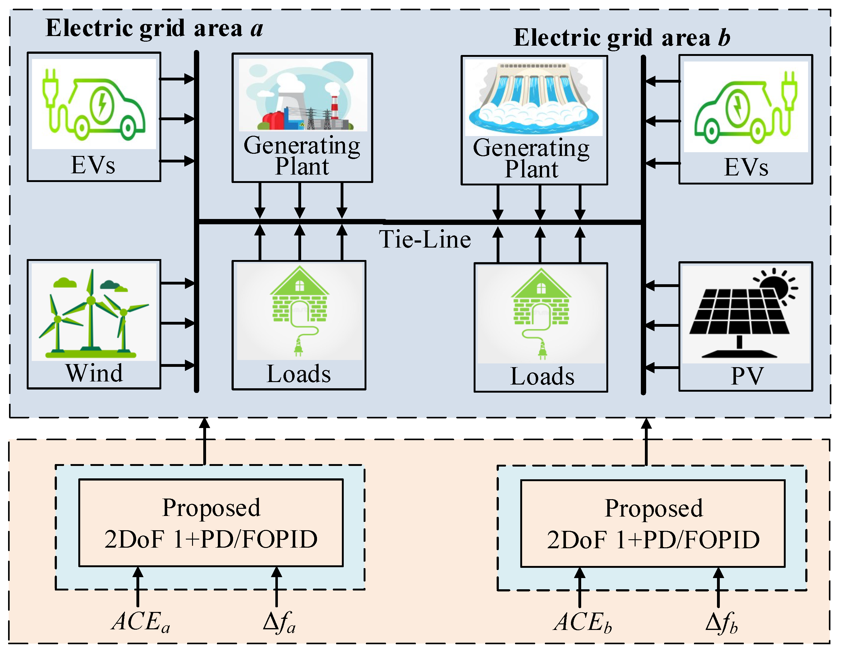
The proposed frequency regulation control methodology is formed using a cascaded 2DoF 1 + PD/FOPID control method, which utilizes two input signals (namely the frequency deviation in each area, and control error in each area (ACE)). The utilization of two different signals is beneficial for the mitigation process of low- and high-frequency existing disturbances.

3.

The proposed frequency regulation methodology using a 2DoF 1 + PD/FOPID controller provides better frequency regulation responses compared with the widely utilized PID, FOPID, and PD/FOPID LFCs, providing better disturbances rejections capabilities. The proposed 2DoF 1 + PD/FOPID structure is capable of mitigating various deviations in area frequency and electrical power grid tie-line power as a direct result of employing two cascaded loops with frequency and ACE signals.

4.

Benefiting from EVs’ batteries in the effective participation in frequency regulation is coordinated through the proposed 2DoF 1 + PD/FOPID structure. Therefore, the proposed 2DoF 1 + PD/FOPID structure reduces the frequency regulation complexities due to employing the centralized frequency regulation structure that coordinates the connected EVs’ batteries and LFC regulator.

5.

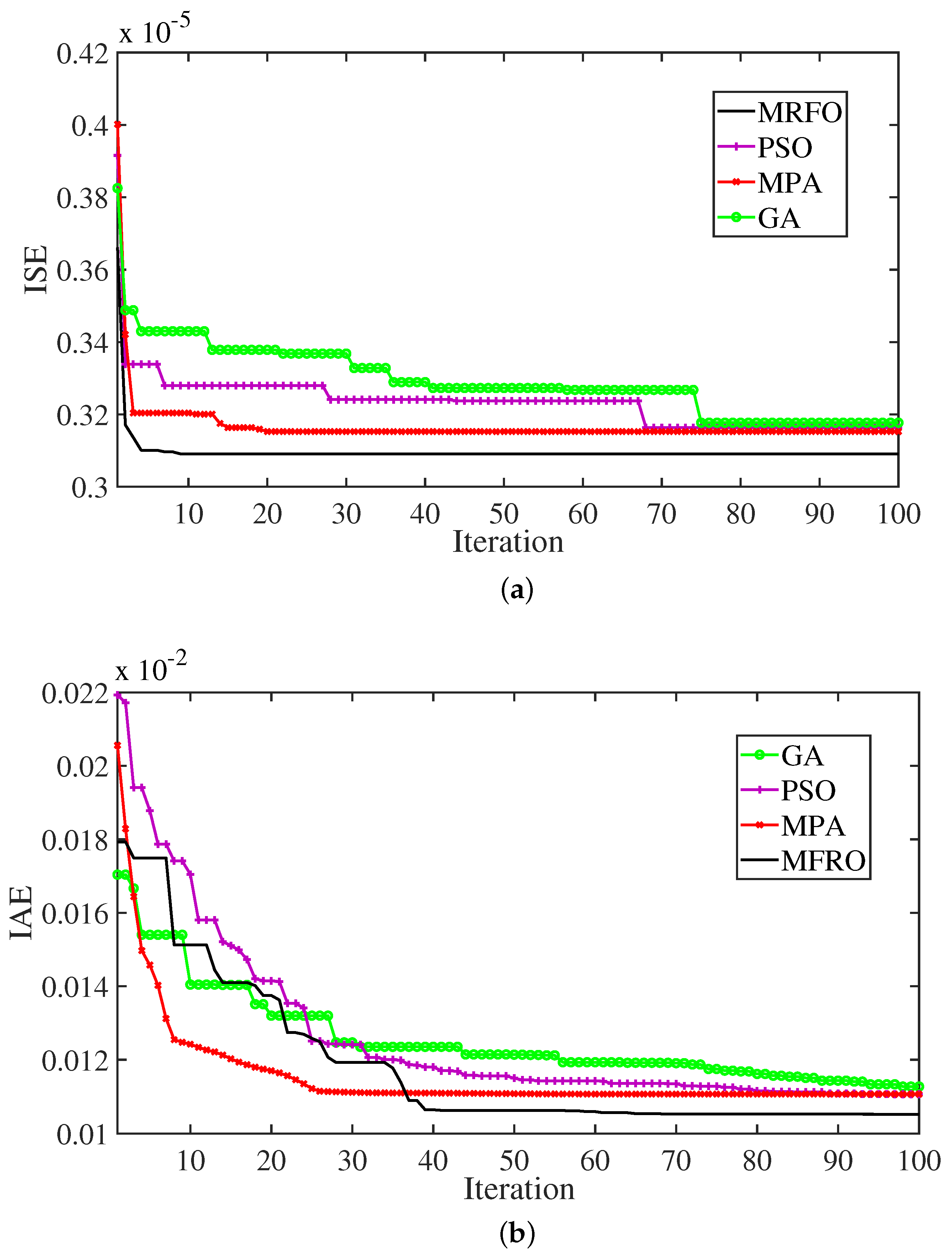
An improved design optimization methodology using the recent manta ray foraging optimization (MRFO) to determine the best parameters for the proposed 2DoF 1 + PD/FOPID frequency regulation. The optimized values of LFCs in different electrical power grids are simultaneously searched using the MRFO optimizer, thus minimizing the desired objectives.

The remainder of the paper is divided as follows: Section 2 provides the mathematical model representations for the interconnected electrical power grids. The proposed 2Dof 1 + PD/FOPID frequency regulation is detailed in Section 3. The proposed design optimization of the 1 + PD/FOPID controller is described in Section 4. Section 5 provides the obtained simulation results of the interconnected two-area electrical power grids with EVs participations and RESs. Finally, the paper’s conclusions are presented in Section 6.

Table 1. Summarized comparison of existing LFC methods and the paper’s contribution.

Ref.	Category	Control Schemes	Characteristics
[16,17,18,19,20,22]	Conventional IO LFC (single input)	I, PI, PID, PIDF	Simple structure and implementation; Low ability to mitigate disturbances; Lower robustness against parameters uncertainty.
[22,39,40,42,43]	Conventional FO LFC (single input)	FOPI, FOPID, FOPIDF	Increased flexibility and number of parameters compared to IO LFC methods; Limited rejection capability of existing disturbances; Lower mitigation of high-frequency deviations.
[24,25,27,28,29,30,32,33]	Cascaded IO LFC (multiple inputs)	PD-PI, PI-PDF, 2DoF-PID, PD-PID, PI-(1 + DD), IPD-(1 + I), FLC-PID	Easy to be implemented; Improved ability to mitigate disturbances; limited number of tunable parameters (only gains can be tuned).
[44,45,46,47,48,49,51,52]	Cascaded FO LFC (multiple inputs)	Cascaded FOPID, 3DOF TID-FOPID, FOID-FOPIDF, FO-IDF, PI-TDF, ID-T, FOPD-PI	Higher number of tunable parameters compared to IO LFC methods; Increased design flexibility compared to other IO-based LFC methods; Enhanced disturbance rejection capability compared to single-input FO LFC methods; Improved mitigation ability of high-frequency deviations.
Proposed	Proposed cascaded FO LFC (multiple inputs)	Proposed cascaded 2DoF 1 + PD/FOPID LFC method	New hybrid (1 + PD) cascaded with FOPID controller for LFC application; Merging the characteristics of IO-based control with the added flexibility of FO control; Simultaneous design optimization process of all tunable parameters, considering connected devices using a powerful MRFO algorithm; Active contribution of EVs in regulating frequency, and this functionality is considered during the design process; High disturbance rejection capability; Better mitigation of high-frequency fluctuations due to using two loops and employing the frequency deviation signal.

Table 1. Summarized comparison of existing LFC methods and the paper’s contribution.

Ref.	Category	Control Schemes	Characteristics
[16,17,18,19,20,22]	Conventional IO LFC (single input)	I, PI, PID, PIDF	Simple structure and implementation; Low ability to mitigate disturbances; Lower robustness against parameters uncertainty.
[22,39,40,42,43]	Conventional FO LFC (single input)	FOPI, FOPID, FOPIDF	Increased flexibility and number of parameters compared to IO LFC methods; Limited rejection capability of existing disturbances; Lower mitigation of high-frequency deviations.
[24,25,27,28,29,30,32,33]	Cascaded IO LFC (multiple inputs)	PD-PI, PI-PDF, 2DoF-PID, PD-PID, PI-(1 + DD), IPD-(1 + I), FLC-PID	Easy to be implemented; Improved ability to mitigate disturbances; limited number of tunable parameters (only gains can be tuned).
[44,45,46,47,48,49,51,52]	Cascaded FO LFC (multiple inputs)	Cascaded FOPID, 3DOF TID-FOPID, FOID-FOPIDF, FO-IDF, PI-TDF, ID-T, FOPD-PI	Higher number of tunable parameters compared to IO LFC methods; Increased design flexibility compared to other IO-based LFC methods; Enhanced disturbance rejection capability compared to single-input FO LFC methods; Improved mitigation ability of high-frequency deviations.
Proposed	Proposed cascaded FO LFC (multiple inputs)	Proposed cascaded 2DoF 1 + PD/FOPID LFC method	New hybrid (1 + PD) cascaded with FOPID controller for LFC application; Merging the characteristics of IO-based control with the added flexibility of FO control; Simultaneous design optimization process of all tunable parameters, considering connected devices using a powerful MRFO algorithm; Active contribution of EVs in regulating frequency, and this functionality is considered during the design process; High disturbance rejection capability; Better mitigation of high-frequency fluctuations due to using two loops and employing the frequency deviation signal.

2. Modelling of Interconnected Electrical Power Grids

2.1. Electrical Power Grid Description

The interconnected electrical power grid using two areas is selected to verify the proposed 1 + PD/FOPID and design optimization method. Figure 1 shows two electrical power grid areas (area a and area b) connected using an AC bus as tie-line between the areas. The electrical power grid area a includes a thermal power plant, local loads, EV batteries, and a wind RES, whereas electrical power grid area b includes a hydraulic power plant, local loads, EV batteries, and a PV RES. It is assumed in the analysis that EVs are equally shared by the two electrical power grids. Each electrical power grid has a frequency regulation controller that controls the power injection of each power/storage devices in the area. The parameters for the studied electrical power grids in this work are taken from [14] and listed in Table 2. Figure 2 presents the complete implemented model of the studied electrical power grid elements with the EV batteries and RESs.

The controlled system consists of the aforementioned two-area interconnected power grids with the connected elements in each area. The input error to be controlled is the ACE signal of each area, and it has to be maintained at a zero reference value. The output of the control method adjusts the contribution of the connected generation and/or energy storage devices to mitigate the frequency changes. When the system has unbalanced generation and loading, this is reflected as an increase/decrease in the system frequency. Therefore, the LFC method mitigates the frequency fluctuations and preserves the frequency deviations at a zero value.

2.2. RES Behaviour Models

In the studied electrical power grids, participation of PV and wind is considered with their intermittency proprieties. They rely on environmental conditions, such as wind speed, solar irradiance levels, and temperatures. For these reasons, continuous tracking is mandatory for the maximum power operating point (MPPT controller), in which, power electronics conversion blocks play a vital role. In addition, they are responsible for grid integration and synchronization of RESs. The outputted powers from RESs are continuously fluctuating due to variations in the weather conditions.

For PV generation, PV outputted power is unpredictable due to its intermittency. This, in turn, results in high-frequency power fluctuations that can lead to severe stability problems in the electrical power grids. In this work, the PV model from [53] is employed for PV power as follows:

$$P_{PV}=\eta {\mathsf{\Phi }}_{solar}{A}_{PV}[1-0.005(T_a+25)]$$

(1)

where $\eta$ stands for PV panel’s conversion efficiency (in %), ${\mathsf{\Phi }}_{solar}$ stands for solar insolation (W/m${}^2$), $A_{PV}$ stands for the area of the PV unit (m${}^2$), and $T_a$ stands for the ambient temperature (°C). The implemented PV configuration model represents a realistic PV power generation model such as in the presented model in [54].

From another side, the outputted mechanical wind power from the turbine possesses high fluctuations resulting from its intermittency characteristics. The wind speed continuously varies, and hence the outputted power differs from instant to another. The calculation of the mechanical power is as follows [55]:

$$P_{wind}=\frac{1}{2}\rho A_r{C}_p{V}_w^3$$

(2)

where $\rho$ stands for the density of air (in kg/m${}^3$), $A_r$ stands for the swept area (in m${}^2$), $C_p$ stands for the power coefficient, and $V_w$ stands for the speed of wind (in m/s). The implemented configuration of the wind power model is based on the realistic representation using the presented modelling in [54].

2.3. EV Behaviour Model

In this study, participation of the installed PV batteries is also considered for the frequency regulation control of the electrical power grids. This, in turn, leads to eliminating the need for additional energy storage capacities in the electrical power grids. The connected EV batteries are charged/discharges based on control signals coming from the electrical power grids. Accordingly, a better performance of the electrical power grid’s reliability, stability, efficiency, and transient response is achieved. In frequency regulation in the electrical power grids, the EV batteries regulate frequencies against the fluctuations resulting from the RESs and connected load proprieties. The used EV battery model is included in Figure 2 for frequency regulation studies in electrical power grids as in [56], in which, Nernst’s equation-based EV battery model determines the dependency of the open circuit battery voltage ($V_{oc}$) on their state of charge ($SOC$) as follows:

$$V_{oc}\left(SOC\right)=V_{nom}+S_p\frac{RT}{F}ln\left(\frac{SOC}{C_{nom}-SOC}\right)$$

(3)

where $V_{oc}\left(SOC\right)$ stands for the $V_{oc}$ dependency on $SOC$, $V_{nom}$ stands for the nominal battery voltage, and $C_{nom}$ stands for the nominal battery capacities of the EVs (in Ah). Furthermore, $S_p$ denotes the sensitivity parameter of the $V_{oc}$ and $SOC$ of the batteries. R and F are the gas and Faraday constants, respectively, and T is the temperature.

2.4. System State Space Model

The studied system in Figure 2 is represented mathematically in Appendix A. The state space-based linear representation is employed for the proposed analysis. The models in Appendix A are collected in the state space model. The general representation of the state space model is modelled as:

$$\dot{x}=Ax+B_1\omega +B_{2}u$$

(4)

$$y=Cx$$

(5)

where x stands for a vector including state variables, y stands for a vector including output states, $\omega$ stands for a vector including the disturbance of a system, and u stands for a vector including the control output. The generation system is modelled using Laplace transform, and this model is employed to define the system state variables vector x. Whereas the load and RESs are considered as disturbances in this model for defining the vector $\omega$. In (4), vectors x and $\omega$ are expressed as:

$$x={\left[\begin{array}{cccccccccc}\Delta f_a& \Delta P_{ga}& \Delta P_{ga1}& \Delta P_{WT}& \Delta f_b& \Delta P_{gb}& \Delta P_{gb1}& \Delta P_{gb2}& \Delta P_{PV}& \Delta P_{tie}\end{array}\right]}^T$$

(6)

$$\omega ={\left[\begin{array}{cccc}\Delta P_{la}& P_{WT}& \Delta P_{lb}& P_{PV}\end{array}\right]}^T$$

(7)

where $\Delta P_{ga}$ and $\Delta P_{ga1}$ are the governor and turbine outputs of the thermal unit in area a, respectively. Whereas $\Delta P_{gb}$, $\Delta P_{gb1}$, and $\Delta P_{gb2}$ are the governor, droop compensation, and penstock turbines outputs of the hydraulic generation in area b, respectively. In (4), vector u includes frequency regulation signals of each electrical power grid $ACE{o}_a$, and $ACE{o}_b$ in addition to the participated power by EVs ($\Delta P_{EVa}$ and $\Delta P_{EVb}$) as follows:

$$u={\left[\begin{array}{cccc}ACE{o}_a& \Delta P_{E{V}_a}& ACE{o}_b& \Delta P_{E{V}_b}\end{array}\right]}^T$$

(8)

The representative matrices in state space modelling in (4), (A, $B_1$, $B_2$, and C) are obtained from the electrical power grid model in Figure 2 and its parameters. They are represented as:

$$A=\left[\begin{array}{cccccccccc}-\frac{D_a}{2H_a}& \frac{1}{2H_a}& 0& \frac{1}{2H_a}& 0& 0& 0& 0& 0& -\frac{1}{2H_a}\\ 0& -\frac{1}{T_t}& \frac{1}{T_t}& 0& 0& 0& 0& 0& 0& 0\\ -\frac{1}{R_a{T}_g}& 0& -\frac{1}{T_g}& 0& 0& 0& 0& 0& 0& 0\\ 0& 0& 0& -\frac{1}{T_{\mathit{WT}}}& 0& 0& 0& 0& 0& 0\\ 0& 0& 0& 0& -\frac{D_b}{2H_b}& \frac{1}{2H_b}& 0& 0& \frac{1}{2H_b}& \frac{1}{2H_b}\\ 0& 0& 0& 0& \frac{2T_R}{R_b{T}_1{T}_2}& -\frac{2}{T_W}& \frac{2T_2+2T_W}{T_2{T}_W}& \frac{2T_R-2T_1}{T_1{T}_2}& 0& 0\\ 0& 0& 0& 0& -\frac{T_R}{R_b{T}_1{T}_2}& 0& -\frac{1}{T_2}& \frac{T_1-T_R}{T_1{T}_2}& 0& 0\\ 0& 0& 0& 0& -\frac{1}{R_b{T}_1}& 0& 0& -\frac{1}{T_1}& 0& 0\\ 0& 0& 0& 0& 0& 0& 0& 0& -\frac{1}{T_{\mathit{PV}}}& 0\\ 2\pi T_{\mathit{tie},\mathit{eq}}& 0& 0& 0& -2\pi T_{\mathit{tie},\mathit{eq}}& 0& 0& 0& 0& 0\end{array}\right]$$

(9)

$$B_1=\left[\begin{array}{cccc}-\frac{1}{2H_a}& 0& 0& 0\\ 0& 0& 0& 0\\ 0& 0& 0& 0\\ 0& \frac{K_{\mathit{WT}}}{T_{\mathit{WT}}}& 0& 0\\ 0& 0& -\frac{1}{2H_b}& 0\\ 0& 0& 0& 0\\ 0& 0& 0& 0\\ 0& 0& 0& 0\\ 0& 0& 0& \frac{K_{\mathit{PV}}}{T_{\mathit{PV}}}\\ 0& 0& 0& 0\end{array}\right]\hspace{1em}, \mathrm{and}\hspace{1em}{B}_2=\left[\begin{array}{cccc}0& -\frac{1}{2H_a}& 0& 0\\ 0& 0& 0& 0\\ \frac{1}{T_g}& 0& 0& 0\\ 0& 0& 0& 0\\ 0& 0& 0& -\frac{1}{2H_b}\\ 0& 0& \frac{2T_R}{T_1{T}_2}& 0\\ 0& 0& \frac{T_R}{T_1{T}_2}& 0\\ 0& 0& \frac{1}{T_1}& 0\\ 0& 0& 0& 0\\ 0& 0& 0& 0\end{array}\right]$$

(10)

$$C=\left[\begin{array}{cccccccccc}1& 0& 0& 0& 0& 0& 0& 0& 0& 0\\ B_{\mathrm{a}}& 0& 0& 0& 0& 0& 0& 0& 0& 1\\ 0& 0& 0& 0& 1& 0& 0& 0& 0& 0\\ 0& 0& 0& 0& B_{\mathrm{b}}& 0& 0& 0& 0& -1\end{array}\right]$$

(11)

Table 2. The electrical power grid parameters for the modelled case study (with $x\in \{a,b\}$), [14].

Symbols	Value
	Area a	Area b
$P_{rx}$ (MW)	1200	1200
$R_x$ (Hz/MW)	2.4	2.4
$B_x$ (MW/Hz)	0.4249	0.4249
Valve min. limit $V_{vlx}$ (p.u.MW)	−0.5	−0.5
Valve max. limit $V_{vux}$ (p.u.MW)	0.5	0.5
$T_g$ (s)	0.08	-
$T_t$ (s)	0.3	-
$T_1$ (s)	-	41.6
$T_2$ (s)	-	0.513
$T_R$ (s)	-	5
$T_w$ (s)	-	1
$H_x$ (p.u.s)	0.0833	0.0833
$D_x$ (p.u./Hz)	0.00833	0.00833
$T_{PV}$ (s)	-	1.3
$K_{PV}$ (s)	-	1
$T_{WT}$ (s)	1.5	-
$K_{WT}$ (s)	1	-
EVs Modelling
Penetration level	5–10%	5–10%
$V_{nom}$ (V)	364.8	364.8
$C_{nom}$ (Ah)	66.2	66.2
$R_s$ (ohms)	0.074	0.074
$R_t$ (ohms)	0.047	0.047
$C_t$ (farad)	703.6	703.6
$RT/F$	0.02612	0.02612
Minimum EVs SOC %	10	10
Maximum EVs SOC %	95	95
Minimum capacity EVs limit (p.u.MW)	−0.1	−0.1
Maximum capacity EVs limit (p.u.MW)	+0.1	+0.1
$C_{batt}$(kWh)	24.15	24.15

Table 2. The electrical power grid parameters for the modelled case study (with $x\in \{a,b\}$), [14].

Symbols	Value
	Area a	Area b
$P_{rx}$ (MW)	1200	1200
$R_x$ (Hz/MW)	2.4	2.4
$B_x$ (MW/Hz)	0.4249	0.4249
Valve min. limit $V_{vlx}$ (p.u.MW)	−0.5	−0.5
Valve max. limit $V_{vux}$ (p.u.MW)	0.5	0.5
$T_g$ (s)	0.08	-
$T_t$ (s)	0.3	-
$T_1$ (s)	-	41.6
$T_2$ (s)	-	0.513
$T_R$ (s)	-	5
$T_w$ (s)	-	1
$H_x$ (p.u.s)	0.0833	0.0833
$D_x$ (p.u./Hz)	0.00833	0.00833
$T_{PV}$ (s)	-	1.3
$K_{PV}$ (s)	-	1
$T_{WT}$ (s)	1.5	-
$K_{WT}$ (s)	1	-
EVs Modelling
Penetration level	5–10%	5–10%
$V_{nom}$ (V)	364.8	364.8
$C_{nom}$ (Ah)	66.2	66.2
$R_s$ (ohms)	0.074	0.074
$R_t$ (ohms)	0.047	0.047
$C_t$ (farad)	703.6	703.6
$RT/F$	0.02612	0.02612
Minimum EVs SOC %	10	10
Maximum EVs SOC %	95	95
Minimum capacity EVs limit (p.u.MW)	−0.1	−0.1
Maximum capacity EVs limit (p.u.MW)	+0.1	+0.1
$C_{batt}$(kWh)	24.15	24.15

Figure 2. Modelling of the various components of the studied electrical power grids.

Figure 2. Modelling of the various components of the studied electrical power grids.

3. The Proposed 2Dof 1 + PD/FOPID Frequency Regulation

3.1. FO-Based Frequency Regulator Representation

The FO-based frequency regulator systems are based on FO calculus and representations of non-integer systems. There are several schemes provided in the literature, such as Grunwald–Letnikov, Riemann–Liouville, and Caputo [57]. The ${\alpha }_{th}$ FO-based derivative for function f between a and t is defined using the Grunwald–Letnikov method:

$$D^{\alpha }{|}_a^t=\underset{h\to 0}{lim}\frac{1}{h^{\alpha }}\sum _{r=0}^{\frac{t-a}{h}}{(-1)}^r\left(\begin{array}{c}n\\ r\end{array}\right)f(t-rh)$$

(12)

where h is the employed step time, and $[·]$ represents the used operator based on integer terms for the Grunwald–Letnikov method. Whereas n should satisfy the condition ($n-1$ $<\alpha <n$). The binomial-based coefficients are represented using:

$$\left(\begin{array}{c}n\\ r\end{array}\right)=\frac{\mathsf{\Gamma }(n+1)}{\mathsf{\Gamma }(r+1)\mathsf{\Gamma }{(n-r+1)}^{\prime }}$$

(13)

where the used gamma function within (13) is usually defined using:

$$\mathsf{\Gamma }(n+1)={\int }_0^{\infty }{t}^{x-1}{e}^{-t}dt$$

(14)

From another side, the Riemann–Liouville method defines FO-based derivatives by avoiding the utilization of the sum and limits, while it uses the integer derivative in addition to the integral representations as follows:

$$D^{\alpha }{|}_a^t=\frac{1}{\mathsf{\Gamma }(n-\alpha )}(\frac{d}{dt}{)}^n{\int }_a^t\frac{f\left(\tau \right)}{{(t-\tau )}^{\alpha -n+1}}d\tau$$

(15)

The Caputo representation for the FO derivative is as follows:

$$D^{\alpha }{|}_a^t=\frac{1}{\mathsf{\Gamma }(n-\alpha )}{\int }_a^t\frac{f^{\left(n\right)}\left(\tau \right)}{{(t-\tau )}^{\alpha -n+1}}d\tau$$

(16)

Generally, the FO non-integer operator $D^{\alpha }{|}_a^t$ can be denoted as follows:

$$D^{\alpha }{|}_a^t=\left\{\begin{array}{cc}\alpha >0\to \frac{{\mathrm{d}}^{\alpha }}{\mathrm{d}{t}^{\alpha }}\hfill & \mathrm{FO}\mathrm{derivative}\hfill \\ \alpha <0\to {\int }_{t_0}^{t_{\mathrm{f}}}\mathrm{d}{t}^{\alpha }\hfill & \mathrm{FO}\mathrm{integral}\hfill \\ \alpha =0\to 1\hfill \end{array}\right.$$

(17)

Implementing FO-based frequency regulators using Oustaloup’s recursive approximation (ORA) has been shown as a suitable digital representation scheme in real-time implementations [57]. The ORA is selected in this paper for FO-based frequency regulator implementations. In which the ${\alpha }^{th}$ derivatives ($s^{\alpha }$) are represented as [57]:

$$s^{\alpha }\approx {\omega }_h^{\alpha }\prod _{k=-N}^N\frac{s+{\omega }_k^z}{s+{\omega }_k^p}$$

(18)

where ${\omega }_{\mathrm{k}}^{\mathrm{p}}$ and ${\omega }_{\mathrm{k}}^{\mathrm{z}}$ stand for the pole/zero locations within the ${\omega }_h$ sequence, and their calculations are as follows:

$${\omega }_k^z={\omega }_b{\left(\frac{{\omega }_h}{{\omega }_b}\right)}^{\frac{k+N+\frac{1-\alpha }{2}}{2N+1}}$$

(19)

$${\omega }_k^p={\omega }_b{\left(\frac{{\omega }_h}{{\omega }_b}\right)}^{\frac{k+N+\frac{1+\alpha }{2}}{2N+1}}$$

(20)

$${\omega }_h^{\alpha }={\left(\frac{{\omega }_h}{{\omega }_b}\right)}^{\frac{-\alpha }{2}}\prod _{k=-N}^N\frac{{\omega }_k^p}{{\omega }_k^z}$$

(21)

where the approximated FO-based frequency regulator operator function possesses a $(2N+1)$ pole/zero number. Therefore, N is related to ORA’s order of representation and equals $(2N+1)$. In this work, ORA is employed for FO-based frequency regulator representation with $(M=5)$ within the frequency range ($\omega \in [{\omega }_{\mathrm{b}},{\omega }_{\mathrm{h}}]$) between $[0.001,1000]$ rad/s.

3.2. Controllers from the Literature

The literature has several proposals of frequency regulation control schemes, including IO- and FO-based frequency controllers. Some existing IO-based frequency regulators include the I, PI, PID, and PIDF LFCs, and their transfer functions (TFs) $C\left(s\right)$ are as follows:

$$\begin{array}{c}{C}_I\left(s\right)=\frac{Y\left(s\right)}{E\left(s\right)}=\frac{K_i}{s}\\ C_{PI}\left(s\right)=\frac{Y\left(s\right)}{E\left(s\right)}=K_p+\frac{K_i}{s}\\ C_{PID}\left(s\right)=\frac{Y\left(s\right)}{E\left(s\right)}=K_p+\frac{K_i}{s}+K_{d}s\\ C_{PIDF}\left(s\right)=\frac{Y\left(s\right)}{E\left(s\right)}=K_p+\frac{K_i}{s}+K_{d}s\frac{N_f}{s+N_f}\end{array}$$

(22)

Whereas FO-based frequency regulators in the literature include the following:

$$\begin{array}{c}{C}_{FOI}\left(s\right)=\frac{Y\left(s\right)}{E\left(s\right)}=\frac{K_i}{s^{\lambda }}\\ C_{FOPI}\left(s\right)=\frac{Y\left(s\right)}{E\left(s\right)}=K_p+\frac{K_i}{s^{\lambda }}\\ C_{FOPID}\left(s\right)=\frac{Y\left(s\right)}{E\left(s\right)}=K_p+\frac{K_i}{s^{\lambda }}+K_d{s}^{\mu }\\ C_{FOPIDF}\left(s\right)=\frac{Y\left(s\right)}{E\left(s\right)}=K_p+\frac{K_i}{s^{\lambda }}+K_d{s}^{\mu }\frac{N_f}{s+N_f}\\ C_{TID}\left(s\right)=\frac{Y\left(s\right)}{E\left(s\right)}=K_t{s}^{-\left(\frac{1}{n}\right)}+\frac{K_i}{s}+K_{d}s\\ C_{FOTID}\left(s\right)=\frac{Y\left(s\right)}{E\left(s\right)}=K_t{s}^{-\left(\frac{1}{n}\right)}+\frac{K_i}{s^{\lambda }}+K_d{s}^{\mu }\\ C_{PFOTID}\left(s\right)=\frac{Y\left(s\right)}{E\left(s\right)}=K_p+K_t{s}^{-\left(\frac{1}{n}\right)}+\frac{K_i}{s^{\lambda }}+K_d{s}^{\mu }\end{array}$$

(23)

It has become evident that each frequency regulator includes a number of tunable parameters to optimize its performance. The number of tunable parameters relies on the employed control scheme.

3.3. Proposed 1 + PD/FOPID Controllers

Figure 3 shows the structure of the proposed 1 + PD/FOPID controller for interconnected electrical power grids. The proposed 1 + PD/FOPID controller uses two cascaded loops using the ACE signal of each electrical power grid in the area in the outer loop and the frequency deviation signal of the area in the inner loop. The 1 + PD is employed for the outer loop and FOPID is employed for the inner loop. Therefore, the proposed 1 + PD/FOPID controller can benefit from both the characteristics of 1 + PDF in the outer loop and the FOPID FO controller in the inner loop. Moreover, the proposed 1 + PD/FOPID controller uses two different inputs signals with different characteristics. That is, the ACE can mitigate low-frequency-related disturbances, while frequency deviation can mitigate high-frequency-related disturbances. Therefore, the proposed 1 + PD/FOPID achieves a fast and robust response, low values of overshoot/undershoot peaks, and a high rate for rejecting disturbances with various frequency scales. The modelling of inputs into the ACE loop ($\left(AC{E}_a\right)$ and $\left(AC{E}_b\right)$) and into the controller inputs ($E_{a1}\left(s\right)$ and $E_{b1}\left(s\right)$) is provided as:

$$\begin{array}{c}{E}_{a1}\left(s\right)=AC{E}_a=\Delta P_{tie}+B_a\Delta f_a\\ E_{b1}\left(s\right)=AC{E}_b=A_{ab}\Delta P_{tie}+B_b\Delta f_b\end{array}$$

(24)

where $\left(A_{ab}\right)$ represents the ratio among the capacities of the electrical power grids’ areas a and b, whereas the outputted signals from $Y_{a1}\left(s\right)$ and $Y_{b1}\left(s\right)$ of the 1 + PD controller’s loop are expressed as:

$$\begin{array}{c}{Y}_{a1}\left(s\right)=[1+K_{p1}+K_{d1}s].E_{a1}\left(s\right)\\ Y_{b1}\left(s\right)=[1+K_{p2}+K_{d2}s].E_{b1}\left(s\right)\end{array}$$

(25)

From (25), each electrical power grid has two parameters for tuning in the outer loop. The electrical power grid in area a has two tunable parameters ($K_{p1}$ and $K_{d1}$), whereas the electrical power grid in area b has $K_{p2}$ and $K_{d2}$ for the tuning process. The output of the outer loop is fed into the inner FOPID loop. The representations of the error signals $E_{a2}\left(s\right)$ and $E_{b2}\left(s\right)$ are as follows:

$$\begin{array}{c}{E}_{a2}\left(s\right)=Y_{a1}\left(s\right)-\Delta P_{tie}-\Delta f_a\\ E_{b2}\left(s\right)=Y_{b1}\left(s\right)-\Delta P_{tie}-\Delta f_b\end{array}$$

(26)

The representations of the FOPID loops are as follows:

$$\begin{array}{c}{Y}_{a2}\left(s\right)=[K_{p3}+\frac{K_{i1}}{s^{{\lambda }_1}}+K_{d3}{s}^{{\mu }_1}].E_{a2}\left(s\right)\\ Y_{b2}\left(s\right)=[K_{p4}+\frac{K_{i2}}{s^{{\lambda }_2}}+K_{d4}{s}^{{\mu }_2}].E_{b2}\left(s\right)\end{array}$$

(27)

From (27), the electric power grid in area a has five tunable control parameters ($K_{p3}$, $K_{i1}$, $K_{d3}$, ${\lambda }_1$ and ${\mu }_1$), and the electrical power grid in area b has $K_{p4}$, $K_{i2}$, $K_{d4}$, ${\lambda }_2$ and ${\mu }_2$ as tunable parameters.

Figure 3. Proposed 1 + PD/FOPID controller.

Figure 3. Proposed 1 + PD/FOPID controller.

4. The Proposed Design Optimization

4.1. MRFO Optimizer

The MRFO is a metaheuristic optimizer that belong to foraging strategies followed by manta rays during the catching process of their prey [58]. It is mainly composed of three foraging processes (chain, cyclone and somersault foraging). During chain foraging, manta rays consider highly concentrated plankton, which represent the desired optimization objectives and tracker. This, in turn, makes them align with the foraging chain. In which, everyone is directed towards food by the manta rays within its front. Then, an updated process of individuals is obtained from the best solution in each iterations. The chain process of foraging is mathematically expressed as [58]:

$$\begin{array}{c}{x}_i^{t+1}=\left\{\begin{array}{c}{x}_i^t+r.(x_{best}^t-x_i^t)+{\omega }_1(x_{best}^t-x_i^t),i=1\hfill \\ x_i^t+r.(x_{i-1}^t-x_i^t)+{\omega }_1(x_{best}^t-x_i^t),i=2:N\hfill \end{array}\right.\hfill \end{array}$$

(28)

where $x_i^t$ stands for the $i^{th}$ position for the current iteration t, r represents a random vector, $x_{best}^t$ stands for best solution in the $t^{th}$ iteration, N is the number of manta rays, and ${\omega }_1$ is the weighting coefficient, expressed as:

$$\begin{array}{c}{\omega }_1=2\times r\times \sqrt{|log(r\left)\right|}\hfill \end{array}$$

(29)

From (28), the individuals’ positions are calculated for all individuals except the first ${(i-1)}^{th}$ individual and the best individual $x_{best}^t$. After plankton patch position determinations using manta rays, a chain is formed by their combination and they swim in a spiral shape towards their prey. Additionally, individuals swim towards the front-sided manta ray. The cyclone foraging process is expressed as:

$$\begin{array}{c}{x}_i^{t+1}=x_{best}+r.(x_{i-1}^t-x_i^t)+e^{b\omega }.cos\left(2\pi \omega \right).(x_{best}-x_i^t)\hfill \\ y_i^{t+1}=y_{best}+r.(y_{i-1}^t-y_i^t)+e^{b\omega }.cos\left(2\pi \omega \right).(y_{best}-y_i^t)\hfill \end{array}$$

(30)

where $\omega$ stands for a random number. Then, the cyclone process foraging is as follows:

$$\begin{array}{c}{x}_i^{t+1}=\left\{\begin{array}{c}{x}_{best}+r.(x_{best}^t-x_i^t)+{\omega }_2(x_{best}^t-x_i^t),i=1\hfill \\ x_{best}+r.(x_{i-1}^t-x_i^t)+{\omega }_2(x_{best}^t-x_i^t),i=2:N\hfill \end{array}\right.\hfill \end{array}$$

(31)

where ${\omega }_2$ represents the weighting factor of cyclone foraging and is determined as:

$$\begin{array}{c}{\omega }_2=2e^{r_1}\left(\frac{T-t+1}{T}\right).sin\left(2\pi r_1\right)\hfill \end{array}$$

(32)

where t stands for the current iteration, T stands for the maximum iterations number, and $r_1$ stands for a random number. The improved exploitation is obtained through the cyclone foraging process to determine the best solution region. This is because all existing manta rays contribute to the food search processes based on their reference positions. Additionally, the exploitation process is also enhanced by forcing the individuals to search for new positions located away from the current best position. The random position in the search space is determined as:

$$\begin{array}{c}{x}_{rand}=Lb+r.(Ub-Lb)\hfill \end{array}$$

(33)

$$\begin{array}{c}{x}_i^{t+1}=\left\{\begin{array}{c}{x}_{rand}+r.(x_{rand}^t-x_i^t)+\beta (x_{rand}^t-x_i^t),i=1\hfill \\ x_{rand}+r.(x_{i-1}^t-x_i^t)+\beta (x_{rand}^t-x_i^t),i=2:N\hfill \end{array}\right.\hfill \end{array}$$

(34)

where $Ub$ and $Lb$ are the upper/lower limits, respectively, of the desired variables, $x_{rand}$ is an assigned random position in the search space. In somersault foraging, the food is recognized in this stage as a hinge. Wherein, each manta ray swims backwards and forwards around the food hinge, and then they tumble to the new position. The somersault foraging process is performed as follows:

$$\begin{array}{c}{x}_i^{t+1}=x_i^t+S.(r_2.x_{best}^t-r_3.x_i^t),i=1,2,...,N\hfill \end{array}$$

(35)

where S is the somersault factor employed to determine the somersault range for the manta rays, and $r_2$ and $r_3$ are random numbers. A flowchart representation of the MRFO stages is shown in Figure 4.

4.2. Design Optimization

The MRFO is proposed in this paper to determine the best parameters for the proposed 1 + PD/FOPID for both electrical power grids. The main driving objectives for the optimum parameters include minimizing the existing fluctuations in the frequency in both areas as well as the tie-line power among the electrical power grids. A measure of frequency deviation ($\Delta f_a$ of area a and $\Delta f_b$ of area b) and tie-line power ($\Delta P_{tie}$ between electrical power grids) is performed and fed into the optimization process. Then, they are combined in a single-objective function to drive the optimization process for simulation time $t_s$ while taking problem constraints into consideration in the process. The employed objective functions can be expressed as follows:

$$ISE=\mathrm{integral}\mathrm{squared}-\mathrm{error}=\underset{0}{\overset{t_s}{\int }}({(\Delta f_a)}^2+{(\Delta f_b)}^2+{(\Delta P_{tie})}^2)\mathrm{d}t$$

(36)

$$ITSE=\mathrm{integral}\mathrm{time}-\mathrm{squared}-\mathrm{error}=\underset{0}{\overset{t_s}{\int }}t.({(\Delta f_a)}^2+{(\Delta f_b)}^2+{(\Delta P_{tie})}^2)\mathrm{d}t$$

(37)

$$IAE=\mathrm{integral}\mathrm{absolute}-\mathrm{error}=\underset{0}{\overset{t_s}{\int }}(abs(\Delta f_a)+abs(\Delta f_b)+abs(\Delta P_{tie}))\mathrm{d}t$$

(38)

$$ITAE=\mathrm{integral}\mathrm{time}-\mathrm{absolute}-\mathrm{error}=\underset{0}{\overset{t_s}{\int }}t.(abs(\Delta f_a)+abs(\Delta f_b)+abs(\Delta P_{tie}))\mathrm{d}t$$

(39)

The ISE and IAE are based on using the integration of the square and absolute error values, respectively, within the simulation time $t_s$. The ISE provides better consideration of the large error values due to the square operation (when errors are more than 1). In addition, IAE provides equal consideration for large and low error values. Whereas ITSE and ITAE consider the time during the integration compared to the ISE and IAE objectives, which leads to lower/zero steady state error compared to ISE and IAE. The four objectives are considered in this paper to provide a comprehensive comparison of the studied controllers.

The proposed design optimization process based on MRFO is summarized in Figure 5. The employed optimization constraints in our proposed design process are:

$$\begin{array}{c}{k}_p^{min}\le k_{p1},k_{p2},k_{p3},k_{p4}\le k_p^{max}\\ k_i^{min}\le k_{i1},k_{i2}\le k_i^{max}\\ k_d^{min}\le k_{d1},k_{d2},k_{d3},k_{d4}\le k_d^{max}\\ {\lambda }^{min}\le {\lambda }_1,{\lambda }_2\le {\lambda }^{max}\\ {\mu }^{min}\le {\mu }_1,{\mu }_2\le {\mu }^{max}\end{array}$$

(40)

where the lower/upper constraints are represented by $min$, and $max$, respectively, for the proposed 1 + PD/FOPID LFC. The used minimum constraints for $k_p^{min}$, $k_i^{min}$, and $k_d^{min}$ were set at zero, and $k_p^{max}$, $k_i^{max}$, and $k_d^{max}$ were set at five during the proposed optimization stages. The set minimum values for ${\lambda }^{min}$ and ${\mu }^{min}$ were zero and for ${\lambda }^{max}$ and ${\mu }^{max}$ were 1.

5. Simulation Results and Performance Verification

The proposed system and proposed design optimization were implemented using the MATLAB R2021a joint m-file and Simulink platforms. The objective function and optimizers were programmed using m-file and linked with Simulink platform. The proposed design optimization process is based on using 20 populations with a maximum of 100 iterations for all the studied optimizers. The same process was used for the design of all the compared controllers for a fair comparison. The two-area electrical power grid system was tested, and the performance of the proposed 1 + PD/FOPID controller was evaluated and compared with the PID, FOPID, and PD/FOPID controllers. Moreover, the convergence performance of the MRFO optimizer was compared with some metaheuristic optimization algorithms from the literature.

The considered optimizers are the GA, PSO, and MPA. The design optimization was made using a personal computer with an Intel Core i7, CPU of 2.9 GHz, and a 64-bit version. Figure 6 compares the ISE and IAE convergence curves of the studied optimizers, whereas Figure 7 shows the ITSE and ITAE comparisons. It has become evident that the MRFO-based design optimization possesses the best convergence with the lowest objective function for all the studied ISE, IAE, ITSE, and ITAE objective functions. In addition, MRFO achieves a very fast conversion with better determination of the control parameters compared with the other studied optimization algorithms. Table 3 summarizes the obtained controllers’ parameters using the proposed design optimization process. The considered test scenarios are organized as follows:

• Scenario (1): Impacts of the stepped load perturbations (SLP);
• Scenario (2): Impacts of multiple SLPs on the two interconnected electrical power grids;
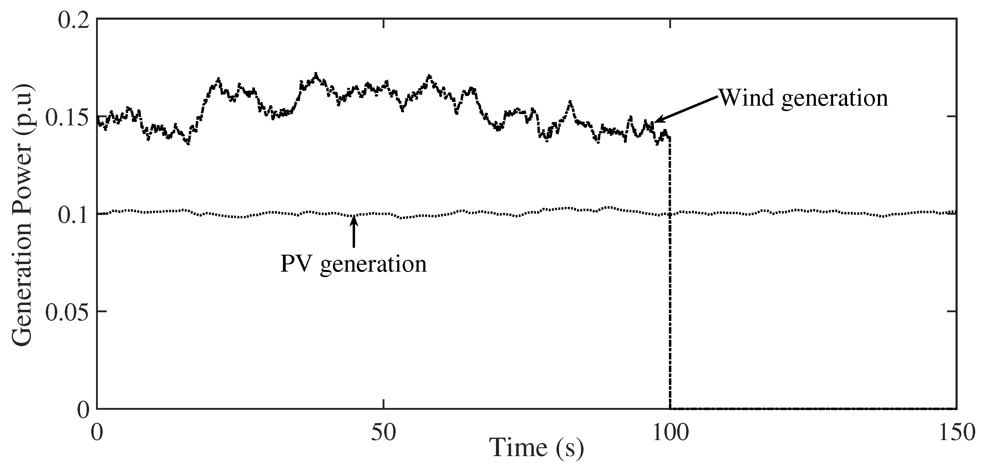
• Scenario (3): Impacts of multiple connection/disconnection of RESs;
• Scenario (4): Impacts of randomly varying loads;
• Scenario (5): Joint impacts of RES fluctuations with various load-type variations.

Table 3. The optimum controllers’ parameters using MRFO design optimization.

Controller	Area	Parameters
		${\mathit{k}}_{\mathit{p}1}$	${\mathit{k}}_{\mathit{p}2}$	${\mathit{k}}_{\mathit{i}1}$	${\mathit{k}}_{\mathit{d}1}$	${\mathit{k}}_{\mathit{d}2}$	${\mathit{\lambda }}_1$	${\mathit{\mu }}_1$
PID	Area a	1.9062	―	1.8547	1.8637	―	―	―
	Area b	0.8808	―	0.2823	0.4233	―	―	―
FOPID	Area a	1.8184	―	1.567	0.9969	―	0.83	0.56
	Area b	1.9809	―	1.189	1.9497	―	0.89	0.73
PD/FOPID	Area a	4.3749	4.9837	1.9231	3.1152	1.6403	0.91	0.76
	Area b	2.5839	4.7702	0.9544	0.7011	3.3158	0.62	0.93
1 + PD/FOPID	Area a	4.5281	3.2751	3.4007	4.2212	4.9497	0.97	0.82
	Area b	3.7113	0.6361	1.6341	4.3158	2.9466	0.77	0.91

Table 3. The optimum controllers’ parameters using MRFO design optimization.

Controller	Area	Parameters
		${\mathit{k}}_{\mathit{p}1}$	${\mathit{k}}_{\mathit{p}2}$	${\mathit{k}}_{\mathit{i}1}$	${\mathit{k}}_{\mathit{d}1}$	${\mathit{k}}_{\mathit{d}2}$	${\mathit{\lambda }}_1$	${\mathit{\mu }}_1$
PID	Area a	1.9062	―	1.8547	1.8637	―	―	―
	Area b	0.8808	―	0.2823	0.4233	―	―	―
FOPID	Area a	1.8184	―	1.567	0.9969	―	0.83	0.56
	Area b	1.9809	―	1.189	1.9497	―	0.89	0.73
PD/FOPID	Area a	4.3749	4.9837	1.9231	3.1152	1.6403	0.91	0.76
	Area b	2.5839	4.7702	0.9544	0.7011	3.3158	0.62	0.93
1 + PD/FOPID	Area a	4.5281	3.2751	3.4007	4.2212	4.9497	0.97	0.82
	Area b	3.7113	0.6361	1.6341	4.3158	2.9466	0.77	0.91

Figure 6. Convergence curves for the proposed design optimization; (a) ISE; (b) IAE.

Figure 6. Convergence curves for the proposed design optimization; (a) ISE; (b) IAE.

Figure 7. Convergence curves for the proposed design optimization; (a) ITSE; (b) ITAE.

Figure 7. Convergence curves for the proposed design optimization; (a) ITSE; (b) ITAE.

5.1. Results of Scenario (1)

Figure 8 shows the obtained results during Scenario (1) with an SLP of 2%. The proposed 1 + PD/FOPID LFC achieves the best transient response compared with the studied controllers. The proposed 1 + PD/FOPID LFC has a maximum undershoot (MU) in $\Delta f_a$ of 0.0018 compared with 0.0101, 0.0061, and 0.0044 under the PID, FOPID, and PD/FOPID, respectively. Moreover, the MU in $\Delta f_b$ was 0.0002 under the proposed 1 + PD/FOPID controller compared with 0.0071, 0.0023, and 0.0016 under the PID, FOPID, and PD/FOPID, respectively. Furthermore, the proposed 1 + PD/FOPID had the lowest settling time (ST) compared with the studied controllers. In addition, the effect of the proposed controller on the thermal, hydraulic, and EV performances is depicted on Figure 9. It can be noted from this figure that the output powers from the thermal power unit and EVs in area a do not exceed their maximum bounds based on different control signals from the frequency variations or area control error. This is reflected as an improvement in the stability behaviour and response of the studied electrical power grids with various expected sudden load changes. For this, the proposed controller succeeded at preserving a better response with subjected load changes compared with the studied controllers.

5.2. Results of Scenario (2)

From another side, Scenario (2) was made using multiple SLPs in different areas. Figure 10 shows the applied load powers in different electrical power grids as a test scenario. Figure 11a–c shows the obtained performance response in this scenario. The response of the frequency and tie-line power transients shows the proposed controller with better transients in all the tested SLP changes in this scenario. From the measured response, the proposed 1 + PD/FOPID has the best frequency deviation response in areas a and b. The proposed 1 + PD/FOPID has an MU in area a of 0.0005 and in area b of 0.0011. Whereas the PID has values of 0.0078 and 0.0103 in areas a and b, respectively; FOPID has values of 0.0051 and 0.0081 in areas a and b, respectively; and PD/FOPID has values of 0.0037 and 0.00581 in areas a and b, respectively. Therefore, the proposed 1 + PD/FOPID achieves the lowest peaks during this scenario. Furthermore, the superior impact of the proposed controller on the performance of the hydraulic generation unit and EVs outputs and its static of charge can be seen in Figure 12, which shows that both of them can regulate the system frequency without exceeding their maximum limits. In addition, it can be observed that there is a cross-coupling between the areas during the transient state, and hence each area produces its own power at a steady state.

5.3. Results at Scenario (3)

In this scenario, multiple RES connections/disconnections have been made to test the proposed controller. Figure 13 shows the PV and wind powers in this scenario. The wind is connected at time 30 s and disconnected at time 80 s. Whereas the PV power is connected at time 50 s. In addition, an SLP is made at the start of the scenario. The obtained results are shown in Figure 14a–c for this scenario. It can be seen that connecting/disconnecting wind/PV affects the response of the system due to its participation level. The proposed 1 + PD/FOPID has the best performance metrics in this scenario, and the PIF has the worst response. For instance, the obtained MO values in area a at 30 s are 0.1202, 0.0596, 0.0456, and 0.0085 for the PID, FOPID, PPD/FOPID, and proposed 1 + PD/FOPID LFC, respectively. The measured performance metrics for all the studied scenarios are shown in Table 4. In which, a performance enhancement is observed when using the proposed control and design optimization method.

5.4. Results at Scenario (4)

An important factor to be considered is the characteristics of the connected electrical load in the electrical power grids. The load varies all day, and hence so too do the expected different demands of power in each moment. These variations are often reflected as fluctuations in the operating frequency of the electrical power grids. Therefore, in this tested scenario, a randomly changing electrical loading is considered as shown in Figure 15. The associated results for this scenario are shown in Figure 16. It can be seen that the proposed 1 + PD/FOPID has the lowest peak fluctuations with varying load profiles. Whereas the PID-based LFC has the highest level of fluctuations during this level. The PD/FOPID comes in second place in terms of improving the electrical power grid response; this followed by the response of the FOPID control.

5.5. Results at Scenario (5)

The interconnected electrical power grids are subjected to joint intermittency of the connected RESs with the connected electrical loading. In this scenario, the domestic and industrial load profiles are considered and studied as shown in Figure 17. Additionally, the fluctuated RESs are included in this scenario with their participation levels and connection/disconnection events in the scenario, as shown in Figure 18. At time 0 s, all the renewable sources and loads are connected, which represents the worst-case scenario to test all the studied controllers and the proposed design optimization method. Figure 19 presents the obtained results in this scenario. The PID at the start of scenario with all RESs and loading step has 0.0927 MO in $\Delta f_a$ of area a and 0.1463 MO in $\Delta f_b$ of area b. Furthermore, regarding the deviations in $\Delta P_{tie}$, the PID has an MU of 0.0461 in this scenario. Therefore, it has the lowest performance of the four studied controllers. From another side, the proposed controller has an MU of 0.0334 and 0.0879 in $\Delta f_a$, and $\Delta f_b$, respectively. In addition, the proposed control has deviations in $\Delta P_{tie}$ of 0.0026 in this scenario. Therefore, the best performance is achieved through the proposed 1 + PD/FOPID LFC method. A full measure of system performance during the five scenarios through various metrics is detailed in Table 4.

Table 4. Measurements of the settling time (ST), peak undershoot (PU), and peak overshoot (PO) for the studied scenarios (where FU stands for a fluctuated condition.

Scenario	Controller	$\Delta {\mathit{f}}_1$			$\Delta {\mathit{f}}_2$			$\Delta {\mathit{P}}_{\mathit{t}\mathit{i}\mathit{e}}$
		PO	PU	ST (s)	PO	PU	ST (s)	PO	PU	ST (s)
No. 1 at 0 s	PID	0.0008	0.0101	13	0.0011	0.0071	9	0.0006	0.0027	19
	FOPID	0.0015	0.0061	11	0.0014	0.0023	11	0.0001	0.0023	16
	PD/FOPID	0.0002	0.0044	8	-	0.0016	10	0.0004	0.0014	10
	1 + PD/FOPID	0.0001	0.0018	4	-	0.0002	3	-	$9.3\times {10}^{-5}$	3
No. 2 at 30 s	PID	0.0003	0.0078	>20 s	0.0005	0.0103	>20 s	0.0035	0.0001	>20 s
	FOPID	0.0006	0.0051	19	0.0006	0.0081	>20 s	0.0031	0.0009	>20 s
	PD/FOPID	-	0.0037	22	0.0012	0.0058	19	0.0029	0.0005	20
	1 + PD/FOPID	-	0.0005	7	-	0.0011	5	0.0003	-	6
No. 3 at 30 s	PID	0.1202	0.0111	FU	0.0739	0.0209	FU	0.0264	0.0039	FU
	FOPID	0.0596	0.0155	FU	0.0236	0.0132	FU	0.0243	0.0058	FU
	PD/FOPID	0.0456	0.0174	13	0.0205	0.0043	11	0.0194	0.0012	FU
	1 + PD/FOPID	0.0085	0.0021	7	0.0031	-	5	0.0015	-	5
No. 4	PID	0.0569	0.0534	FU	0.0537	0.0608	FU	0.0179	0.0192	FU
	FOPID	0.0239	0.0272	FU	0.0219	0.0209	FU	0.0139	0.0124	FU
	PD/FOPID	0.0094	0.0088	FU	0.0076	0.0092	FU	0.0094	0.0089	FU
	1 + PD/FOPID	0.0017	0.0015	FU	0.0012	0.0013	FU	0.0007	0.0006	FU
No. 5 at 0 s	PID	0.0927	0.0073	FU	0.1463	0.0127	FU	0.0077	0.0461	FU
	FOPID	0.0527	0.0004	FU	0.0879	0.0092	FU	0.0019	0.0285	FU
	PD/FOPID	0.0471	0.0141	FU	0.0711	0.0065	FU	0.0022	0.0221	FU
	1 + PD/FOPID	0.0334	-	15	0.0191	-	19	-	0.0026	23

Table 4. Measurements of the settling time (ST), peak undershoot (PU), and peak overshoot (PO) for the studied scenarios (where FU stands for a fluctuated condition.

Scenario	Controller	$\Delta {\mathit{f}}_1$			$\Delta {\mathit{f}}_2$			$\Delta {\mathit{P}}_{\mathit{t}\mathit{i}\mathit{e}}$
		PO	PU	ST (s)	PO	PU	ST (s)	PO	PU	ST (s)
No. 1 at 0 s	PID	0.0008	0.0101	13	0.0011	0.0071	9	0.0006	0.0027	19
	FOPID	0.0015	0.0061	11	0.0014	0.0023	11	0.0001	0.0023	16
	PD/FOPID	0.0002	0.0044	8	-	0.0016	10	0.0004	0.0014	10
	1 + PD/FOPID	0.0001	0.0018	4	-	0.0002	3	-	$9.3\times {10}^{-5}$	3
No. 2 at 30 s	PID	0.0003	0.0078	>20 s	0.0005	0.0103	>20 s	0.0035	0.0001	>20 s
	FOPID	0.0006	0.0051	19	0.0006	0.0081	>20 s	0.0031	0.0009	>20 s
	PD/FOPID	-	0.0037	22	0.0012	0.0058	19	0.0029	0.0005	20
	1 + PD/FOPID	-	0.0005	7	-	0.0011	5	0.0003	-	6
No. 3 at 30 s	PID	0.1202	0.0111	FU	0.0739	0.0209	FU	0.0264	0.0039	FU
	FOPID	0.0596	0.0155	FU	0.0236	0.0132	FU	0.0243	0.0058	FU
	PD/FOPID	0.0456	0.0174	13	0.0205	0.0043	11	0.0194	0.0012	FU
	1 + PD/FOPID	0.0085	0.0021	7	0.0031	-	5	0.0015	-	5
No. 4	PID	0.0569	0.0534	FU	0.0537	0.0608	FU	0.0179	0.0192	FU
	FOPID	0.0239	0.0272	FU	0.0219	0.0209	FU	0.0139	0.0124	FU
	PD/FOPID	0.0094	0.0088	FU	0.0076	0.0092	FU	0.0094	0.0089	FU
	1 + PD/FOPID	0.0017	0.0015	FU	0.0012	0.0013	FU	0.0007	0.0006	FU
No. 5 at 0 s	PID	0.0927	0.0073	FU	0.1463	0.0127	FU	0.0077	0.0461	FU
	FOPID	0.0527	0.0004	FU	0.0879	0.0092	FU	0.0019	0.0285	FU
	PD/FOPID	0.0471	0.0141	FU	0.0711	0.0065	FU	0.0022	0.0221	FU
	1 + PD/FOPID	0.0334	-	15	0.0191	-	19	-	0.0026	23

6. Conclusions

An improved fractional-order controller based on a cascaded 1 + PD/FOPID control was proposed in this paper with MRFO-based design optimization to regulate the frequency in interconnected electrical grids. The proposed controller is advantageous at mitigating disturbances at a wide range of frequencies due to employing two cascaded control loops. Additionally, the employment of the MRFO and design optimization process leads to simultaneous design and determination of the best control parameters. The proposed 1 + PD/FOPID and MRFO-based design optimization were implemented and simulated in MATLAB. Various scenarios of load power changes and renewable power connection/interconnection scenarios were considered in the performance investigation. In addition, the PID, FOPID and PD/FOPID LFCs were compared with the proposed controller. Results verify the reduced peak overshoot and settling times under the proposed 1 + PD/FOPID LFC compared with the studied controllers. Future research includes the use of more practical modelling of electric power systems (integer and fractional-order modelling), stability analysis with system non-linearities, and comprehensive comparisons of existing LFC methods.

References

1. Blaabjerg, F.; Yang, Y.; Kim, K.A.; Rodriguez, J. Power Electronics Technology for Large-Scale Renewable Energy Generation. Proc. IEEE 2023, 111, 335–355. [Google Scholar] [CrossRef]
2. Biswas, S.; Mahata, S.; Roy, P.K.; Chatterjee, K. Application of Empirical Bode Analysis for Delay-Margin Evaluation of Fractional-Order PI Controller in a Renewable Distributed Hybrid System. Fractal Fract. 2023, 7, 119. [Google Scholar] [CrossRef]
3. Sami, I.; Ullah, S.; Khan, L.; Al-Durra, A.; Ro, J.S. Integer and Fractional-Order Sliding Mode Control Schemes in Wind Energy Conversion Systems: Comprehensive Review, Comparison, and Technical Insight. Fractal Fract. 2022, 6, 447. [Google Scholar] [CrossRef]
4. Salama, H.S.; Said, S.M.; Aly, M.; Vokony, I.; Hartmann, B. Studying Impacts of Electric Vehicle Functionalities in Wind Energy-Powered Utility Grids With Energy Storage Device. IEEE Access 2021, 9, 45754–45769. [Google Scholar] [CrossRef]
5. Alilou, M.; Azami, H.; Oshnoei, A.; Mohammadi-Ivatloo, B.; Teodorescu, R. Fractional-Order Control Techniques for Renewable Energy and Energy-Storage-Integrated Power Systems: A Review. Fractal Fract. 2023, 7, 391. [Google Scholar] [CrossRef]
6. Daraz, A.; Malik, S.A.; Basit, A.; Aslam, S.; Zhang, G. Modified FOPID Controller for Frequency Regulation of a Hybrid Interconnected System of Conventional and Renewable Energy Sources. Fractal Fract. 2023, 7, 89. [Google Scholar] [CrossRef]
7. Fayek, H.H. 5G Poor and Rich Novel Control Scheme Based Load Frequency Regulation of a Two-Area System with 100% Renewables in Africa. Fractal Fract. 2020, 5, 2. [Google Scholar] [CrossRef]
8. Ahmed, E.M.; Mohamed, E.A.; Selim, A.; Aly, M.; Alsadi, A.; Alhosaini, W.; Alnuman, H.; Ramadan, H.A. Improving load frequency control performance in interconnected power systems with a new optimal high degree of freedom cascaded FOTPID-TIDF controller. Ain Shams Eng. J. 2023, 14, 102207. [Google Scholar] [CrossRef]
9. Mohamed, E.A.; Aly, M.; Elmelegi, A.; Ahmed, E.M.; Watanabe, M.; Said, S.M. Enhancement the Frequency Stability and Protection of Interconnected Microgrid Systems Using Advanced Hybrid Fractional Order Controller. IEEE Access 2022, 10, 111936–111961. [Google Scholar] [CrossRef]
10. Kavikumar, R.; Kwon, O.M.; Lee, S.H.; Sakthivel, R. Input-output finite-time IT2 fuzzy dynamic sliding mode control for fractional-order nonlinear systems. Nonlinear Dyn. 2022, 108, 3745–3760. [Google Scholar] [CrossRef]
11. Kavikumar, R.; Sakthivel, R.; Kwon, O.M.; Selvaraj, P. Robust tracking control design for fractional-order interval type-2 fuzzy systems. Nonlinear Dyn. 2022, 107, 3611–3628. [Google Scholar] [CrossRef]
12. Gheisarnejad, M.; Khooban, M.H.; Dragicevic, T. The Future 5G Network-Based Secondary Load Frequency Control in Shipboard Microgrids. IEEE J. Emerg. Sel. Top. Power Electron. 2020, 8, 836–844. [Google Scholar] [CrossRef]
13. Gheisarnejad, M.; Karimaghaie, P.; Boudjadar, J.; Khooban, M.H. Real-Time Cellular Wireless Sensor Testbed for Frequency Regulation in Smart Grids. IEEE Sens. J. 2019, 19, 11656–11665. [Google Scholar] [CrossRef]
14. Ahmed, E.M.; Selim, A.; Alnuman, H.; Alhosaini, W.; Aly, M.; Mohamed, E.A. Modified Frequency Regulator Based on TIλ-TDμFF Controller for Interconnected Microgrids with Incorporating Hybrid Renewable Energy Sources. Mathematics 2022, 11, 28. [Google Scholar] [CrossRef]
15. Aly, M.; Mohamed, E.A.; Noman, A.M.; Ahmed, E.M.; El-Sousy, F.F.M.; Watanabe, M. Optimized Non-Integer Load Frequency Control Scheme for Interconnected Microgrids in Remote Areas with High Renewable Energy and Electric Vehicle Penetrations. Mathematics 2023, 11, 2080. [Google Scholar] [CrossRef]
16. Dahab, Y.A.; Abubakr, H.; Mohamed, T.H. Adaptive Load Frequency Control of Power Systems Using Electro-Search Optimization Supported by the Balloon Effect. IEEE Access 2020, 8, 7408–7422. [Google Scholar] [CrossRef]
17. Ewais, A.M.; Elnoby, A.M.; Mohamed, T.H.; Mahmoud, M.M.; Qudaih, Y.; Hassan, A.M. Adaptive frequency control in smart microgrid using controlled loads supported by real-time implementation. PLoS ONE 2023, 18, e0283561. [Google Scholar] [CrossRef]
18. Arora, K.; Kumar, A.; Kamboj, V.K.; Prashar, D.; Shrestha, B.; Joshi, G.P. Impact of Renewable Energy Sources into Multi Area Multi-Source Load Frequency Control of Interrelated Power System. Mathematics 2021, 9, 186. [Google Scholar] [CrossRef]
19. Gupta, D.K.; Soni, A.K.; Jha, A.V.; Mishra, S.K.; Appasani, B.; Srinivasulu, A.; Bizon, N.; Thounthong, P. Hybrid Gravitational–Firefly Algorithm-Based Load Frequency Control for Hydrothermal Two-Area System. Mathematics 2021, 9, 712. [Google Scholar] [CrossRef]
20. Yousri, D.; Babu, T.S.; Fathy, A. Recent methodology based Harris Hawks optimizer for designing load frequency control incorporated in multi-interconnected renewable energy plants. Sustain. Energy Grids Netw. 2020, 22, 100352. [Google Scholar] [CrossRef]
21. Salama, H.S.; Magdy, G.; Bakeer, A.; Vokony, I. Adaptive coordination control strategy of renewable energy sources, hydrogen production unit, and fuel cell for frequency regulation of a hybrid distributed power system. Prot. Control Mod. Power Syst. 2022, 7, 34. [Google Scholar] [CrossRef]
22. Shabani, H.; Vahidi, B.; Ebrahimpour, M. A robust PID controller based on imperialist competitive algorithm for load-frequency control of power systems. ISA Trans. 2013, 52, 88–95. [Google Scholar] [CrossRef] [PubMed]
23. Youssef, A.R.; Mallah, M.; Ali, A.; Shaaban, M.F.; Mohamed, E.E.M. Enhancement of Microgrid Frequency Stability Based on the Combined Power-to-Hydrogen-to-Power Technology under High Penetration Renewable Units. Energies 2023, 16, 3377. [Google Scholar] [CrossRef]
24. Sahu, R.K.; Panda, S.; Rout, U.K.; Sahoo, D.K. Teaching learning based optimization algorithm for automatic generation control of power system using 2-DOF PID controller. Int. J. Electr. Power Energy Syst. 2016, 77, 287–301. [Google Scholar] [CrossRef]
25. Kouba, N.E.Y.; Menaa, M.; Hasni, M.; Boudour, M. Optimal load frequency control based on artificial bee colony optimization applied to single, two and multi-area interconnected power systems. In Proceedings of the 2015 3rd International Conference on Control, Engineering Information Technology (CEIT), Tlemcen, Algeria, 25–27 May 2015. [Google Scholar] [CrossRef]
26. Abid, S.; El-Rifaie, A.M.; Elshahed, M.; Ginidi, A.R.; Shaheen, A.M.; Moustafa, G.; Tolba, M.A. Development of Slime Mold Optimizer with Application for Tuning Cascaded PD-PI Controller to Enhance Frequency Stability in Power Systems. Mathematics 2023, 11, 1796. [Google Scholar] [CrossRef]
27. Zhang, G.; Daraz, A.; Khan, I.A.; Basit, A.; Khan, M.I.; Ullah, M. Driver Training Based Optimized Fractional Order PI-PDF Controller for Frequency Stabilization of Diverse Hybrid Power System. Fractal Fract. 2023, 7, 315. [Google Scholar] [CrossRef]
28. Singh, B.; Slowik, A.; Bishnoi, S.K.; Sharma, M. Frequency Regulation Strategy of Two-Area Microgrid System with Electric Vehicle Support Using Novel Fuzzy-Based Dual-Stage Controller and Modified Dragonfly Algorithm. Energies 2023, 16, 3407. [Google Scholar] [CrossRef]
29. Mohanty, B.; Panda, S.; Hota, P. Controller parameters tuning of differential evolution algorithm and its application to load frequency control of multi-source power system. Int. J. Electr. Power Energy Syst. 2014, 54, 77–85. [Google Scholar] [CrossRef]
30. Dash, P.; Saikia, L.C.; Sinha, N. Automatic generation control of multi area thermal system using Bat algorithm optimized PD–PID cascade controller. Int. J. Electr. Power Energy Syst. 2015, 68, 364–372. [Google Scholar] [CrossRef]
31. Raju, M.; Saikia, L.C.; Sinha, N. Automatic generation control of a multi-area system using ant lion optimizer algorithm based PID plus second order derivative controller. Int. J. Electr. Power Energy Syst. 2016, 80, 52–63. [Google Scholar] [CrossRef]
32. Latif, A.; Hussain, S.M.S.; Das, D.C.; Ustun, T.S. Optimization of Two-Stage IPD-(1I) Controllers for Frequency Regulation of Sustainable Energy Based Hybrid Microgrid Network. Electronics 2021, 10, 919. [Google Scholar] [CrossRef]
33. Gheisarnejad, M. An effective hybrid harmony search and cuckoo optimization algorithm based fuzzy PID controller for load frequency control. Appl. Soft Comput. 2018, 65, 121–138. [Google Scholar] [CrossRef]
34. Prakash, S.; Sinha, S. Simulation based neuro-fuzzy hybrid intelligent PI control approach in four-area load frequency control of interconnected power system. Appl. Soft Comput. 2014, 23, 152–164. [Google Scholar] [CrossRef]
35. Latif, A.; Paul, M.; Das, D.C.; Hussain, S.M.S.; Ustun, T.S. Price Based Demand Response for Optimal Frequency Stabilization in ORC Solar Thermal Based Isolated Hybrid Microgrid under Salp Swarm Technique. Electronics 2020, 9, 2209. [Google Scholar] [CrossRef]
36. Hussain, I.; Das, D.C.; Latif, A.; Sinha, N.; Hussain, S.S.; Ustun, T.S. Active power control of autonomous hybrid power system using two degree of freedom PID controller. Energy Rep. 2022, 8, 973–981. [Google Scholar] [CrossRef]
37. Bakeer, A.; Magdy, G.; Chub, A.; Jurado, F.; Rihan, M. Optimal Ultra-Local Model Control Integrated with Load Frequency Control of Renewable Energy Sources Based Microgrids. Energies 2022, 15, 9177. [Google Scholar] [CrossRef]
38. Yakout, A.H.; AboRas, K.M.; Kotb, H.; Alharbi, M.; Shouran, M.; Samad, B.A. A Novel Ultra Local Based-Fuzzy PIDF Controller for Frequency Regulation of a Hybrid Microgrid System with High Renewable Energy Penetration and Storage Devices. Processes 2023, 11, 1093. [Google Scholar] [CrossRef]
39. Ayas, M.S.; Sahin, E. FOPID controller with fractional filter for an automatic voltage regulator. Comput. Electr. Eng. 2021, 90, 106895. [Google Scholar] [CrossRef]
40. Fathy, A.; Alharbi, A.G. Recent Approach Based Movable Damped Wave Algorithm for Designing Fractional-Order PID Load Frequency Control Installed in Multi-Interconnected Plants With Renewable Energy. IEEE Access 2021, 9, 71072–71089. [Google Scholar] [CrossRef]
41. Latif, A.; Hussain, S.S.; Das, D.C.; Ustun, T.S.; Iqbal, A. A review on fractional order (FO) controllers’ optimization for load frequency stabilization in power networks. Energy Rep. 2021, 7, 4009–4021. [Google Scholar] [CrossRef]
42. Singh, K.; Amir, M.; Ahmad, F.; Refaat, S.S. Enhancement of Frequency Control for Stand-Alone Multi-Microgrids. IEEE Access 2021, 9, 79128–79142. [Google Scholar] [CrossRef]
43. Zaheeruddin; Singh, K. Load frequency regulation by de-loaded tidal turbine power plant units using fractional fuzzy based PID droop controller. Appl. Soft Comput. 2020, 92, 106338. [Google Scholar] [CrossRef]
44. Oshnoei, S.; Aghamohammadi, M.; Oshnoei, S.; Oshnoei, A.; Mohammadi-Ivatloo, B. Provision of Frequency Stability of an Islanded Microgrid Using a Novel Virtual Inertia Control and a Fractional Order Cascade Controller. Energies 2021, 14, 4152. [Google Scholar] [CrossRef]
45. Peddakapu, K.; Srinivasarao, P.; Mohamed, M.; Arya, Y.; Kishore, D.K. Stabilization of frequency in Multi-Microgrid system using barnacle mating Optimizer-based cascade controllers. Sustain. Energy Technol. Assess. 2022, 54, 102823. [Google Scholar] [CrossRef]
46. Arya, Y.; Kumar, N.; Dahiya, P.; Sharma, G.; Çelik, E.; Dhundhara, S.; Sharma, M. Cascade-I ΛDμN controller design for AGC of thermal and hydro-thermal power systems integrated with renewable energy sources. IET Renew. Power Gener. 2021, 15, 504–520. [Google Scholar] [CrossRef]
47. Malik, S.; Suhag, S. A Novel SSA Tuned PI-TDF Control Scheme for Mitigation of Frequency Excursions in Hybrid Power System. Smart Sci. 2020, 8, 202–218. [Google Scholar] [CrossRef]
48. Priyadarshani, S.; Subhashini, K.R.; Satapathy, J.K. Pathfinder algorithm optimized fractional order tilt-integral-derivative (FOTID) controller for automatic generation control of multi-source power system. Microsyst. Technol. 2020, 27, 23–35. [Google Scholar] [CrossRef]
49. Oshnoei, A.; Khezri, R.; Muyeen, S.M.; Oshnoei, S.; Blaabjerg, F. Automatic Generation Control Incorporating Electric Vehicles. Electr. Power Compon. Syst. 2019, 47, 720–732. [Google Scholar] [CrossRef]
50. Sahu, R.K.; Panda, S.; Biswal, A.; Sekhar, G.C. Design and analysis of tilt integral derivative controller with filter for load frequency control of multi-area interconnected power systems. ISA Trans. 2016, 61, 251–264. [Google Scholar] [CrossRef]
51. Elkasem, A.H.; Khamies, M.; Hassan, M.H.; Nasrat, L.; Kamel, S. Utilizing controlled plug-in electric vehicles to improve hybrid power grid frequency regulation considering high renewable energy penetration. Int. J. Electr. Power Energy Syst. 2023, 152, 109251. [Google Scholar] [CrossRef]
52. Ahmed, M.; Magdy, G.; Khamies, M.; Kamel, S. Modified TID controller for load frequency control of a two-area interconnected diverse-unit power system. Int. J. Electr. Power Energy Syst. 2022, 135, 107528. [Google Scholar] [CrossRef]
53. Khokhar, B.; Dahiya, S.; Parmar, K.P.S. A Robust Cascade Controller for Load Frequency Control of a Standalone Microgrid Incorporating Electric Vehicles. Electr. Power Compon. Syst. 2020, 48, 711–726. [Google Scholar] [CrossRef]
54. Das, D.C.; Roy, A.; Sinha, N. GA based frequency controller for solar thermal–diesel–wind hybrid energy generation/energy storage system. Int. J. Electr. Power Energy Syst. 2012, 43, 262–279. [Google Scholar] [CrossRef]
55. Ray, P.K.; Mohanty, S.R.; Kishor, N. Proportional–integral controller based small-signal analysis of hybrid distributed generation systems. Energy Convers. Manag. 2011, 52, 1943–1954. [Google Scholar] [CrossRef]
56. Ahmed, E.M.; Mohamed, E.A.; Elmelegi, A.; Aly, M.; Elbaksawi, O. Optimum Modified Fractional Order Controller for Future Electric Vehicles and Renewable Energy-Based Interconnected Power Systems. IEEE Access 2021, 9, 29993–30010. [Google Scholar] [CrossRef]
57. Micev, M.; Ćalasan, M.; Oliva, D. Fractional Order PID Controller Design for an AVR System Using Chaotic Yellow Saddle Goatfish Algorithm. Mathematics 2020, 8, 1182. [Google Scholar] [CrossRef]
58. Zhao, W.; Zhang, Z.; Wang, L. Manta ray foraging optimization: An effective bio-inspired optimizer for engineering applications. Eng. Appl. Artif. Intell. 2020, 87, 103300. [Google Scholar] [CrossRef]
Figure 1. Structure of studied electrical power grids and the proposed 1 + PD/FOPID control.
Fractalfract 07 00603 g001
Figure 4. Flowchart representation of the MRFO stages.
Fractalfract 07 00603 g004
Figure 5. Proposed design optimization of the 1 + PD/FOPID controller.
Fractalfract 07 00603 g005
Figure 8. Performance evaluations with an SLP of 2%. Scenario (1): (a Δ f a ; (b Δ f b ; (c Δ P t i e .
Fractalfract 07 00603 g008
Figure 9. EV participation in Scenario (1): (a) EV output power; (b) EV battery SOC; (c) generator output power.
Fractalfract 07 00603 g009
Figure 10. Load profiles at multiple SLPs in Scenario (2).
Fractalfract 07 00603 g010
Figure 11. Performance evaluations at multiple SLPs Scenario (2): (a Δ f a ; (b Δ f b ; (c Δ P t i e .
Fractalfract 07 00603 g011aFractalfract 07 00603 g011b
Figure 12. EV participation in Scenario (2): (a) EV output power; (b) EV battery SOC; (c) generator output power.
Fractalfract 07 00603 g012aFractalfract 07 00603 g012b
Figure 13. Load and RES generation profiles in Scenario (3).
Fractalfract 07 00603 g013
Figure 14. Performance evaluations for RES changes in Scenario (3): (a Δ f a ; (b Δ f b ; (c Δ P t i e .
Fractalfract 07 00603 g014aFractalfract 07 00603 g014b
Figure 15. Random load change profiles of Scenario (4).
Fractalfract 07 00603 g015
Figure 16. Performance evaluations at random load changes in Scenario (4): (a Δ f a ; (b Δ f b ; (c Δ P t i e .
Fractalfract 07 00603 g016
Figure 17. Load profiles at high RES participation in Scenario (5).
Fractalfract 07 00603 g017
Figure 18. PV and wind generation profiles at high RES participation in Scenario (5).
Fractalfract 07 00603 g018
Figure 19. Performance evaluations at high RES participation in Scenario (5): (a Δ f a ; (b Δ f b ; (c Δ P t i e .
Fractalfract 07 00603 g019
Disclaimer/Publisher’s Note: The statements, opinions and data contained in all publications are solely those of the individual author(s) and contributor(s) and not of MDPI and/or the editor(s). MDPI and/or the editor(s) disclaim responsibility for any injury to people or property resulting from any ideas, methods, instructions or products referred to in the content.