Local Fractional Homotopy Perturbation Method for Solving Coupled Sine-Gordon Equations in Fractal Domain

Abstract

In this paper, the coupled local fractional sine-Gordon equations are studied in the range of local fractional derivative theory. The study of exact solutions of nonlinear coupled systems is of great significance for understanding complex physical phenomena in reality. The main method used in this paper is the local fractional homotopy perturbation method, which is used to analyze the exact traveling wave solutions of generalized nonlinear systems defined on the Cantor set in the fractal domain. The fractal wave with fractal dimension $\epsilon =ln2/ln3$ is numerically simulated. Through numerical simulation, we find that the obtained solutions are of great significance to explain some practical physical problems.

1. Introduction

In the field of science, most problems and phenomena are nonlinear, especially in mechanics [1], plasma physics [2], plasma waves, heat conduction [3] and chemical physics. Many scholars have made accurate analysis of various nonlinear problems and put forward some methods to solve them. Examples include Backlund transformation [4], bilinear method [5], sine-cosine method [6], Adomian decomposition method [7], variational iteration method [8], exp-function method [9] and homotopy perturbation method (HPM) [10,11]. We conclude that HPM is the most effective and simplest method to solve nonlinear problems.

HPM was first proposed by He [12]. He introduced the HPM into the solution of nonlinear wave equations. The advantage of this method is that it does not depend on the small parameters in the topology. There is a homotopy technique in topology that we can use to construct a homotopy with one parameter, and it is considered to be a small parameter [13]. HPM is widely used in nonlinear wave equations. It is used to solve water wave theory [14], heat conduction [15] and diffusion problems [16].

In recent years, Yang [17] redefined and generalized the local order, and constructed a complete framework of the local order defined on Cantor sets. Local fractions are usually used to describe various fractal problems in real life and science. Local fraction theory is a new efficient algorithm to obtain the exact solution of a local fraction problem. The solution of this theory is defined on the Cantor set. Yang used the local fractional homotopy perturbation (LFHP) method to solve the wave equations involving Cantor sets [18]. Zhang used the same method to solve the heat conduction equation in the fractal system [19]. The results show that the theoretical method is accurate and feasible, and has strong practical significance.

A coupled system of nonlinear equations is as follows:

$$\left\{\begin{array}{c}{\psi }_{tt}-{\psi }_{xx}=-{\delta }^{2}sin(\psi -\omega ),\hfill \\ {\omega }_{tt}-c^2{\omega }_{xx}=sin(\psi -\omega ),\hfill \end{array}\right.$$

(1)

where $\delta , c$ are arbitrary constants, and $\delta >0, c>0$.

The above coupled equations are an extension of the Frenkel–Kontorova model [20]. It simulates one-dimensional nonlinear wave processes in two-component media [21]. Coupled sine-Gordon equations with $c=1$ were proposed to describe the open states in a DNA model. The coupled sine-Gordon equations can describe the propagation of optical pulses in fiber waveguide [22]. It can also describe long wave motion in shallow water. In recent years, many scholars have studied and analyzed the system (1). Salas gives its exact soliton solution and periodic solution [23]. Zhao et al. obtained the exact solution of the above equation by using the hyperbolic auxiliary function method [24]. Hosseini et al. solved the above coupling equations in nonlinear optics by using an improved Kudryashov method [22].

Our main purpose is to solve the traveling wave solutions of the following coupled local fractional sine-Gordon equations by using the LFHP method.

$$\left\{\begin{array}{c}\frac{{\mathsf{\partial }}^{2\epsilon }\psi }{\mathsf{\partial }{t}^{2\epsilon }}-\frac{{\mathsf{\partial }}^{2\epsilon }\psi }{\mathsf{\partial }{x}^{2\epsilon }}=-{\delta }^2{sin}_{\epsilon }{\left(\psi -\omega \right)}^{\epsilon },\hfill \\ \hfill \\ \frac{{\mathsf{\partial }}^{2\epsilon }\omega }{\mathsf{\partial }{t}^{2\epsilon }}-c^2\frac{{\mathsf{\partial }}^{2\epsilon }\omega }{\mathsf{\partial }{x}^{2\epsilon }}={sin}_{\epsilon }{\left(\psi -\omega \right)}^{\epsilon },\hfill \end{array}\right.$$

(2)

where $\epsilon$ is the fractal dimension and $0<\epsilon \le 1$.

In this paper, the basic idea of the local fractional homotopy perturbation method is introduced and the traveling wave solutions of coupled local fractional sine-Gordon equations are obtained by using this method. The structure is as follows: The Section 2 introduces the basic theory and operation formula of local fractional calculus. The Section 3 introduces the basic idea and operation process of the LFHP method. In Section 4, we obtain the traveling wave solutions of coupled local fractional sinusoidal Gordon equations using the LFHP method, and obtain their wave images using MATLAB. Finally, we summarize the main conclusions in Section 5.

2. Local Fractional Calculus

2.1. Local Fractional Derivatives

Definition 1.

We define $C_{\epsilon }(\mu ,\nu )$ as a set of the nondifferentiable functions. Setting $\mathsf{\Psi }\left(\chi \right)\in C_{\epsilon }(\mu ,\nu )$, local fractional derivative of $\mathsf{\Psi }\left(\chi \right)$ of order $\epsilon (0<\epsilon \le 1)$ at $\chi ={\chi }_0$ is defined by [25]

$$D^{\left(\epsilon \right)}\mathsf{\Psi }\left(\chi \right)={\left.\frac{{\mathrm{d}}^{\epsilon }\mathsf{\Psi }\left(\chi \right)}{\mathrm{d}{\chi }^{\epsilon }}\right|}_{\chi ={\chi }_0}=\underset{\chi \to {\chi }_0}{lim}\frac{{\mathsf{\Delta }}^{\epsilon }\left[\mathsf{\Psi }\left(\chi \right)-\mathsf{\Psi }\left({\chi }_0\right)\right]}{{\left(\chi -{\chi }_0\right)}^{\epsilon }},$$

(3)

where ${\mathsf{\Delta }}^{\epsilon }\left[\mathsf{\Psi }\left(\chi \right)-\mathsf{\Psi }\left({\chi }_0\right)\right]\cong \mathsf{\Gamma }(1+\epsilon )\left[\mathsf{\Psi }\left(\chi \right)-\mathsf{\Psi }\left({\chi }_0\right)\right]$.

In addition, the local higher order fractional partial derivative is defined as

$$\frac{{\mathsf{\partial }}^{k\epsilon }}{\mathsf{\partial }{\chi }^{k\epsilon }}\mathsf{\Psi }(\chi ,\gamma )=\stackrel{k\mathrm{times}}{\overbrace{\frac{{\mathsf{\partial }}^{\epsilon }}{\mathsf{\partial }{\chi }^{\epsilon }}\dots \frac{{\mathsf{\partial }}^{\epsilon }}{\mathsf{\partial }{\chi }^{\epsilon }}}}\mathsf{\Psi }(\chi ,\gamma ).$$

The properties of the local fractional derivative are listed as follows [26]:

$$\begin{array}{cc}& \left(R1\right)D^{\left(\epsilon \right)}\left[\mathsf{\Psi }\left({\chi }_0\right)\pm \Re \left({\chi }_0\right)\right]=D^{\left(\epsilon \right)}\mathsf{\Psi }\left({\chi }_0\right)\pm D^{\left(\epsilon \right)}\Re \left({\chi }_0\right),\hfill \\ \hfill \\ & \left(R2\right)D^{\left(\epsilon \right)}\left[\mathsf{\Psi }\left({\chi }_0\right)\Re \left({\chi }_0\right)\right]=\mathsf{\Psi }\left({\chi }_0\right)D^{\left(\epsilon \right)}\mathsf{\Psi }\left({\chi }_0\right)+\mathsf{\Psi }\left({\chi }_0\right)D^{\left(\epsilon \right)}\Re \left({\chi }_0\right),\hfill \\ \hfill \\ & \left(R3\right)D^{\left(\epsilon \right)}\left[\frac{\mathsf{\Psi }\left({\chi }_0\right)}{\Re \left({\chi }_0\right)}\right]=\frac{\left\{\left[D^{\left(\epsilon \right)}\mathsf{\Psi }\left({\chi }_0\right)\right]\Re \left({\chi }_0\right)-\mathsf{\Psi }\left({\chi }_0\right)\left[D^{\left(\epsilon \right)}\Re \left({\chi }_0\right)\right]\right\}}{{\Re }^2\left({\chi }_0\right)},\hfill \end{array}$$

where $\Re \left({\chi }_0\right)\ne 0$, and $\mathsf{\Psi }\left({\chi }_0\right),\Re \left({\chi }_0\right)\in C_{\epsilon }(\mu ,\nu )$.

2.2. Local Fractional Integral

Definition 2.

The local fraction integral of $\mathsf{\Phi }\left(\chi \right)$ is defined as [27]

$$\begin{array}{cc}{}_{\alpha }{I}_{\beta }^{\left(\epsilon \right)}\mathsf{\Phi }\left(\chi \right)=\hfill & \frac{1}{\mathsf{\Gamma }(1+\epsilon )}{\int }_{\mu }^{\nu }\mathsf{\Phi }\left(\chi \right){\left(\mathrm{d}\chi \right)}^{\epsilon }=\frac{1}{\mathsf{\Gamma }(1+\epsilon )}\underset{\mathsf{\Delta }{\chi }_{\sigma }\to 0}{lim}\sum _{\sigma =0}^{N-1}\mathsf{\Phi }\left({\chi }_{\sigma }\right){\left(\mathsf{\Delta }{\chi }_{\sigma }\right)}^{\epsilon },\hfill \end{array}$$

(4)

where $\mathsf{\Phi }\left(\chi \right)\in C_{\epsilon }(\mu ,\nu )$, and $\mathsf{\Delta }{\chi }_{\sigma }={\chi }_{\sigma +1}-{\chi }_{\sigma }$ with ${\chi }_0=\alpha <{\chi }_1<\cdots <{\chi }_{N-1}<{\chi }_N=\beta$.

The properties of the local fractional integral are as follows:

$$\begin{array}{cc}& \left(S1\right)\frac{1}{\mathsf{\Gamma }(1+\epsilon )}{\int }_{\mu }^x\left[D^{\left(\epsilon \right)}\mathsf{\Phi }\left(\chi \right)\right]{\left(d\chi \right)}^{\epsilon }=\phi \left(x\right)-\mathsf{\Phi }\left(\mu \right),\hfill \\ & \left(S2\right)D^{\left(\epsilon \right)}\left[\frac{1}{\mathsf{\Gamma }(1+\epsilon )}{\int }_{\alpha }^x\mathsf{\Phi }\left(\chi \right){\left(d\chi \right)}^{\epsilon }\right]=\mathsf{\Phi }\left(x\right).\hfill \end{array}$$

2.3. Basic Operation

It defines the generalized function by [28]

$$\begin{array}{cc}& E_{\epsilon }\left({\chi }^{\epsilon }\right)=\sum _{\kappa =0}^{\infty }\frac{{\chi }^{\kappa \epsilon }}{\mathsf{\Gamma }(1+\kappa \epsilon )},\hfill \\ & {sin}_{\epsilon }\left({\chi }^{\epsilon }\right)=\sum _{\kappa =0}^{\infty }\frac{{(-1)}^{\kappa }{\chi }^{(2\kappa +1)\epsilon }}{\mathsf{\Gamma }(1+(2\kappa +1\left)\epsilon \right)},\hfill \\ & {cos}_{\epsilon }\left({\chi }^{\epsilon }\right)=\sum _{\kappa =0}^{\infty }\frac{{(-1)}^{\kappa }{\chi }^{2\kappa \epsilon }}{\mathsf{\Gamma }(1+2\kappa \epsilon )},\hfill \\ & {sinh}_{\epsilon }\left({\chi }^{\epsilon }\right)=\frac{E_{\epsilon }\left({\chi }^{\epsilon }\right)-E_{\epsilon }\left(-{\chi }^{\epsilon }\right)}{2}=\sum _{\kappa =0}^{\infty }\frac{{\chi }^{(2\kappa +1)\epsilon }}{\mathsf{\Gamma }(1+(2\kappa +1\left)\epsilon \right)},\hfill \\ & {cosh}_{\epsilon }\left({\chi }^{\epsilon }\right)=\frac{E_{\epsilon }\left({\chi }^{\epsilon }\right)+E_{\epsilon }\left(-{\chi }^{\epsilon }\right)}{2}=\sum _{\kappa =0}^{\infty }\frac{{\chi }^{2\kappa \epsilon }}{\mathsf{\Gamma }(1+2\kappa \epsilon )}.\hfill \end{array}$$

Local fractional calculus has the following properties [28]

$$\begin{array}{cc}& \frac{d^{\epsilon }}{d{\chi }^{\epsilon }}{E}_{\epsilon }\left(C{\chi }^{\epsilon }\right)=C{E}_{\epsilon }\left(C{\chi }^{\epsilon }\right),\frac{d^{\epsilon }}{d{\chi }^{\epsilon }}{sin}_{\epsilon }\left(C{\chi }^{\epsilon }\right)=C{cos}_{\epsilon }\left(C{\chi }^{\epsilon }\right),\hfill \\ & \frac{d^{\epsilon }}{d{\chi }^{\epsilon }}{cos}_{\epsilon }\left(C{\chi }^{\epsilon }\right)=-C{sin}_{\epsilon }\left(C{\chi }^{\epsilon }\right),\frac{d^{\epsilon }}{d{\chi }^{\epsilon }}{sinh}_{\epsilon }\left(C{\chi }^{\epsilon }\right)=C{cosh}_{\epsilon }\left(C{\chi }^{\epsilon }\right),\hfill \\ & \frac{d^{\epsilon }}{d{\chi }^{\epsilon }}{cosh}_{\epsilon }\left(C{\chi }^{\epsilon }\right)=C{sinh}_{\epsilon }\left(C{\chi }^{\epsilon }\right),\frac{d^{\epsilon }}{d{\chi }^{\epsilon }}\frac{{\chi }^{\kappa \epsilon }}{\mathsf{\Gamma }(1+\kappa \epsilon )}=\frac{{\chi }^{(\kappa -1)\epsilon }}{\mathsf{\Gamma }(1+(\kappa -1\left)\epsilon \right)},\hfill \end{array}$$

and

$$\begin{array}{cc}& {}_0{I}_{\chi }^{\left(\epsilon \right)}\frac{{\chi }^{\kappa \epsilon }}{\mathsf{\Gamma }(1+\kappa \epsilon )}=\frac{{\chi }^{(\kappa +1)\epsilon }}{\mathsf{\Gamma }(1+(\kappa +1\left)\epsilon \right)}.\hfill \end{array}$$

3. Local Fractional Homotopy Perturbation Method

For a given class of local fractional differential equations,

$$L_{\sigma }\left({\phi }^{\sigma }\right)=0,\phi \in R,$$

(5)

where $L_{\sigma }$ is a local fractional differential operator.

First, let us set up a homotopy mapping [18]:

$$\begin{array}{cc}{H}_{\sigma }(\phi ,\rho )=\hfill & \left(1-{\rho }^{\sigma }\right)\left(L_{\sigma }\left({\phi }^{\sigma }\right)-L_{\sigma }\left({\phi }_0^{\sigma }\right)\right)+{\rho }^{\sigma }{L}_{\sigma }\left({\phi }^{\sigma }\right),\hfill \\ \hfill & \phi \in R,\rho \in [0,1],\hfill \end{array}$$

(6)

or

$$\begin{array}{cc}{H}_{\sigma }(\phi ,\rho )=\hfill & L_{\sigma }\left({\phi }^{\sigma }\right)-L_{\sigma }\left({\phi }_0^{\sigma }\right)+{\rho }^{\sigma }{L}_{\sigma }\left({\phi }_0^{\sigma }\right),\hfill \\ \hfill & \phi \in R,\rho \in [0,1],\hfill \end{array}$$

(7)

where $\rho$ is an imbedding parameter and ${\phi }_0$ is an initial approximation of Equation (5).

Let $H_{\sigma }(\phi ,\rho )=0$, then we can obtain, from Equation (6),

$$\begin{array}{c}{H}_{\sigma }(u,0)=L_{\sigma }\left({\phi }^{\sigma }\right)-L_{\sigma }\left({\phi }_0^{\sigma }\right)=0;\\ H_{\sigma }(\phi ,1)=L_{\sigma }\left({\phi }_0^{\sigma }\right)=0.\end{array}$$

(8)

According to the homotopy perturbation theory, $\rho$ can be treated as a small parameter. Suppose that the solution $\phi$ of Equation (6) can be expressed as a power series of $\rho$

$${\phi }^{\sigma }={\phi }_0^{\sigma }+{\rho }^{\sigma }{\phi }_1^{\sigma }+{\rho }^{2\sigma }{\phi }_2^{\sigma }+{\rho }^{2\sigma }{\phi }_2^{\sigma }+\dots =\sum _{i=0}^n{\rho }^{i\sigma }{\phi }_i^{\sigma }.$$

(9)

Substituting Equation (9) into Equation (6), we obtain

$$H_{\sigma }\left(\sum _{i=0}^n{\rho }^i{\phi }_i,p\right)=\left(1-{\rho }^{\sigma }\right)\left(L_{\sigma }\left(\sum _{i=0}^n{\rho }^i{\phi }_i\right)-L_{\sigma }\left({\phi }_0\right)\right)+{\rho }^{\sigma }{L}_{\sigma }\left(\sum _{i=0}^n{\rho }^i{\phi }_i\right).$$

An extended form of $L_{\sigma }\left({\phi }^{\sigma }\right)$ [19]

$$\begin{array}{cc}{L}_{\sigma }\left({\phi }^{\sigma }\right)\hfill & =L_{\sigma }\left({\phi }_0^{\sigma }\right)+\frac{d^{\sigma }\left(L_{\sigma }\left({\phi }_0^{\sigma }\right)\right)}{d{\phi }^{\sigma }}\frac{\left({\sum }_{i=0}^n{\rho }^i{\phi }_i-{\phi }_0\right)}{\mathsf{\Gamma }(1+\sigma )}+O\left({\left(\sum _{i=0}^n{\rho }^i{\phi }_i-{\phi }_0\right)}^{\sigma }\right)\hfill \\ & =L_{\sigma }\left({\phi }_0^{\sigma }\right)+\frac{d^{\sigma }\left(L_{\sigma }\left({\phi }_0^{\sigma }\right)\right)}{d{\phi }^{\sigma }}\frac{\left({\sum }_{i=0}^n{\rho }^{i\sigma }{\phi }_i^{\sigma }-{\phi }_0^{\sigma }\right)}{\mathsf{\Gamma }(1+\sigma )}+O\left({\left(\sum _{i=0}^n{\rho }^i{\phi }_i-{\phi }_0\right)}^{\sigma }\right),\hfill \end{array}$$

such that

$$\begin{array}{cc}\hfill & H_{\sigma }(\phi ,\rho ,\sigma )\hfill \\ \hfill & ={(1-\rho )}^{\sigma }\left(L_{\sigma }\left({\phi }^{\sigma }\right)-L_{\sigma }\left({\phi }_0^{\sigma }\right)\right)+{\rho }^{\sigma }{L}_{\sigma }\left({\phi }^{\sigma }\right)\hfill \\ \hfill & ={(1-\rho )}^{\sigma }\left(L_{\sigma }\left({\phi }_0^{\sigma }\right)+\frac{d^{\sigma }\left(L_{\sigma }\left({\phi }_0^{\sigma }\right)\right)}{d{\phi }^{\sigma }}\frac{\left({\sum }_{i=0}^n{\rho }^{i\sigma }{\phi }_i^{\sigma }-{\phi }_0^{\sigma }\right)}{\mathsf{\Gamma }(1+\sigma )}+O\left({\left(\sum _{i=0}^n{\rho }^i{\phi }_i-{\phi }_0\right)}^{\sigma }\right)-L_{\sigma }\left({\phi }_0^{\sigma }\right)\right)\hfill \\ \hfill & +{\rho }^{\sigma }\left(L_{\sigma }\left({\phi }_0^{\sigma }\right)+\frac{d^{\sigma }\left(L_{\sigma }\left({\phi }_0^{\sigma }\right)\right)}{d{\phi }^{\sigma }}\frac{\left({\sum }_{j=0}^n{\rho }^{j\sigma }{\phi }_i^{\sigma }-{\phi }_0^{\sigma }\right)}{\mathsf{\Gamma }(1+\sigma )}+O\left({\left(\sum _{j=0}^n{\rho }^j{\phi }_i-{\phi }_0\right)}^{\sigma }\right)\right),\hfill \end{array}$$

(10)

which reduces to

$$\begin{array}{cc}{H}_{\sigma }(\phi ,0)\hfill & =L_{\sigma }\left({\phi }^{\sigma }\right)-L_{\sigma }\left({\phi }_0^{\sigma }\right)\hfill \\ & =\frac{{\mathrm{d}}^{\sigma }\left(L_{\sigma }\left({\phi }_0^{\sigma }\right)\right)}{\mathrm{d}{\phi }^{\sigma }}\frac{{\left({\sum }_{i=0}^n{\rho }^i{\phi }_i-{\phi }_0\right)}^{\sigma }}{\mathsf{\Gamma }(1+\sigma )}+\frac{{\mathrm{d}}^{2\sigma }\left(L_{\sigma }\left({\phi }_0^{\sigma }\right)\right)}{\mathrm{d}{\phi }^{2\sigma }}\frac{{\left({\sum }_{i=0}^n{\rho }^i{\phi }_i-{\phi }_0\right)}^{2\sigma }}{\mathsf{\Gamma }(1+2\sigma )}\hfill \\ & +\frac{{\mathrm{d}}^{n\sigma }\left(L_{\sigma }\left({\phi }_0^{\sigma }\right)\right)}{\mathrm{d}{\phi }^{n\sigma }}\frac{{\left({\sum }_{i=0}^n{\rho }^i{\phi }_i-{\phi }_0\right)}^{n\sigma }}{\mathsf{\Gamma }(1+n\sigma )}+\dots =0,\hfill \end{array}$$

and

$$\begin{array}{cc}& H_{\sigma }(\phi ,1)=L_{\sigma }\left({\phi }^{\sigma }\right)\hfill \\ & =L_{\sigma }\left({\phi }_0^{\sigma }\right)+\frac{{\mathrm{d}}^{\sigma }\left(L_{\sigma }\left({\phi }_0^{\sigma }\right)\right)}{\mathrm{d}{\phi }^{\sigma }}\frac{{\left({\sum }_{i=0}^n{\rho }^i{\phi }_i-{\phi }_0\right)}^{\sigma }}{\mathsf{\Gamma }(1+\sigma )}+\frac{{\mathrm{d}}^{2\sigma }\left(L_{\sigma }\left({\phi }_0^{\sigma }\right)\right)}{\mathrm{d}{\phi }^{2\sigma }}\frac{{\left({\sum }_{i=0}^n{\rho }^i{\phi }_i-{\phi }_0\right)}^{2\sigma }}{\mathsf{\Gamma }(1+2\sigma )}\hfill \\ & +\frac{{\mathrm{d}}^{n\sigma }\left(L_{\sigma }\left({\phi }_0^{\sigma }\right)\right)}{\mathrm{d}{\phi }^{n\sigma }}\frac{{\left({\sum }_{i=0}^n{\rho }^i{\phi }_i-{\phi }_0\right)}^{n\sigma }}{\mathsf{\Gamma }(1+n\sigma )}+\dots =0.\hfill \end{array}$$

Using the expression Equation (10), we find that

$${\rho }^{0\sigma }:L_{\sigma }\left({\phi }^{\sigma }\right)-L_{\sigma }\left({\phi }_0^{\sigma }\right)=0,$$

$${\rho }^{1\sigma }:\frac{{\mathrm{d}}^{\sigma }\left(L_{\sigma }\left({\phi }_0^{\sigma }\right)\right)}{\mathrm{d}{\phi }^{\sigma }}\frac{{\phi }_1^{\sigma }}{\mathsf{\Gamma }(1+\sigma )}+L_{\sigma }\left({\phi }_0^{\sigma }\right)=0,$$

$${\rho }^{2\sigma }:\frac{{\mathrm{d}}^{\sigma }\left(L_{\sigma }\left({\phi }_0^{\sigma }\right)\right)}{\mathrm{d}{\phi }^{\sigma }}\frac{{\phi }_2^{\sigma }}{\mathsf{\Gamma }(1+\sigma )}+\frac{{\mathrm{d}}^{2\sigma }\left(L_{\sigma }\left({\phi }_0^{\sigma }\right)\right)}{\mathrm{d}{\phi }^{2\sigma }}\frac{{\phi }_1^{2\sigma }}{\mathsf{\Gamma }(1+2\sigma )}=0.$$

when $\rho \to 1$, we have the approximate solution of the form:

$${\phi }^{\sigma }=\underset{\rho \to 1}{lim}\sum _{i=0}^n{\rho }^{i\sigma }{\phi }_i^{\sigma }=\sum _{i=0}^n{\phi }_i^{\sigma }.$$

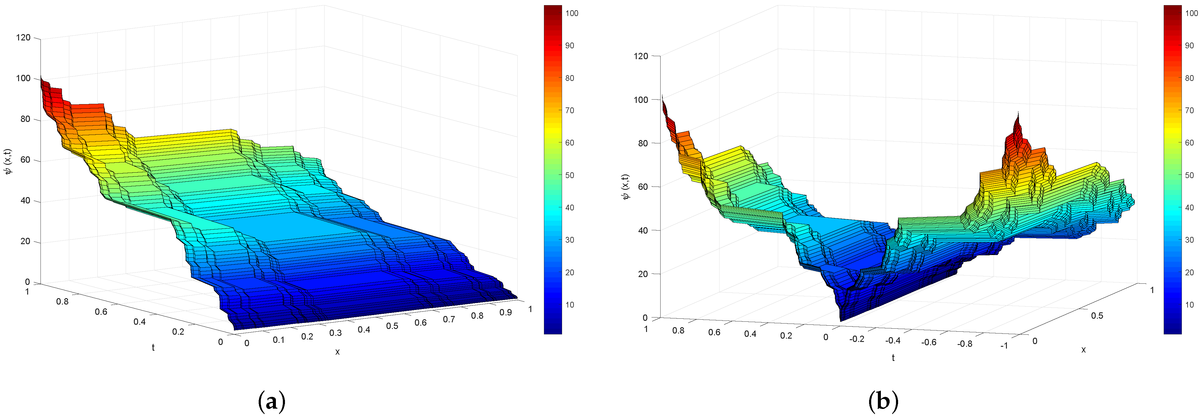
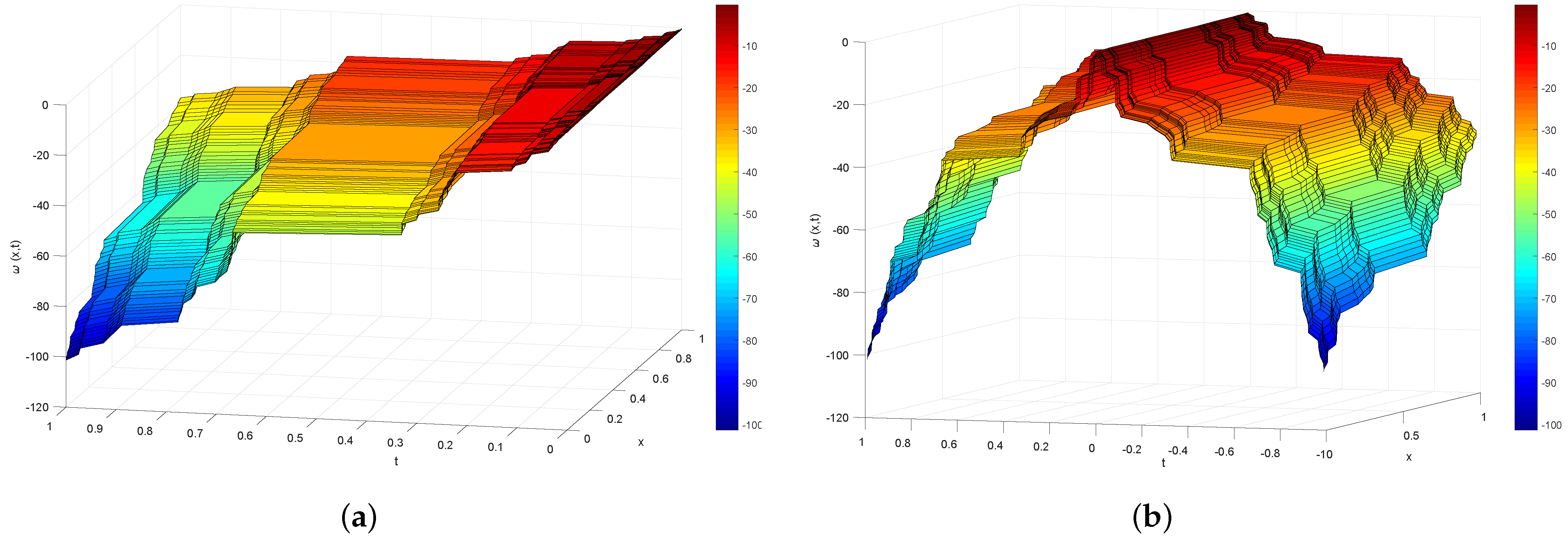
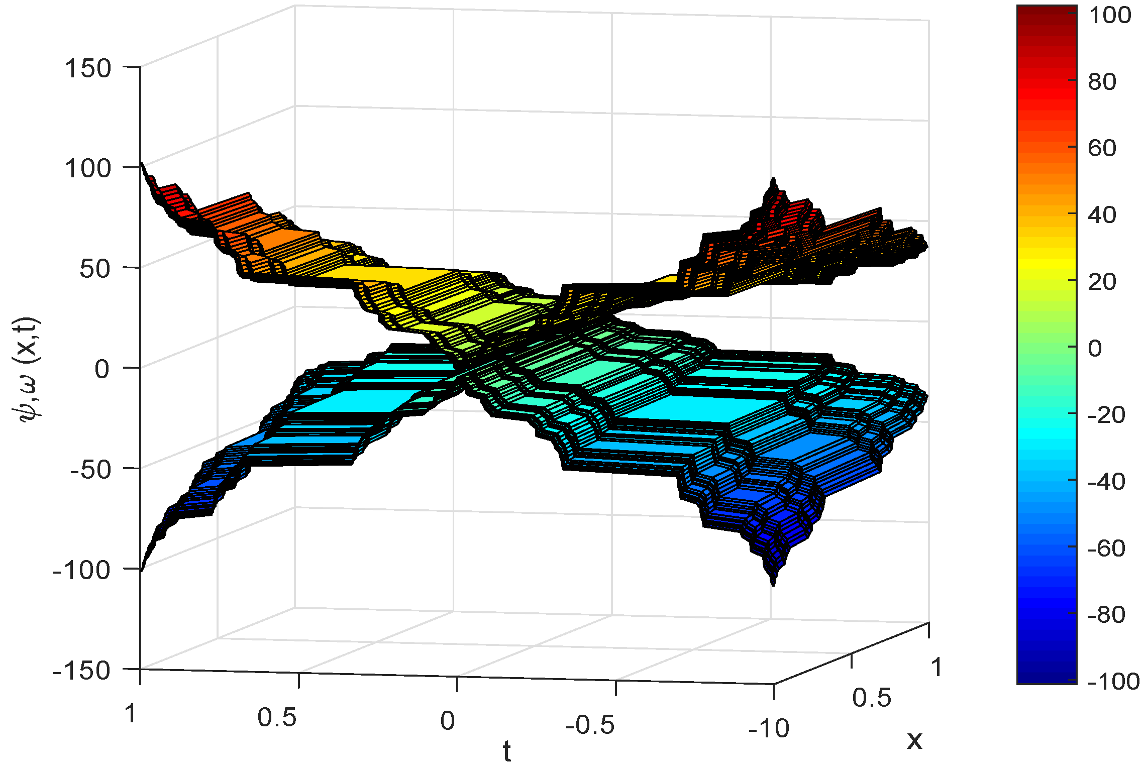
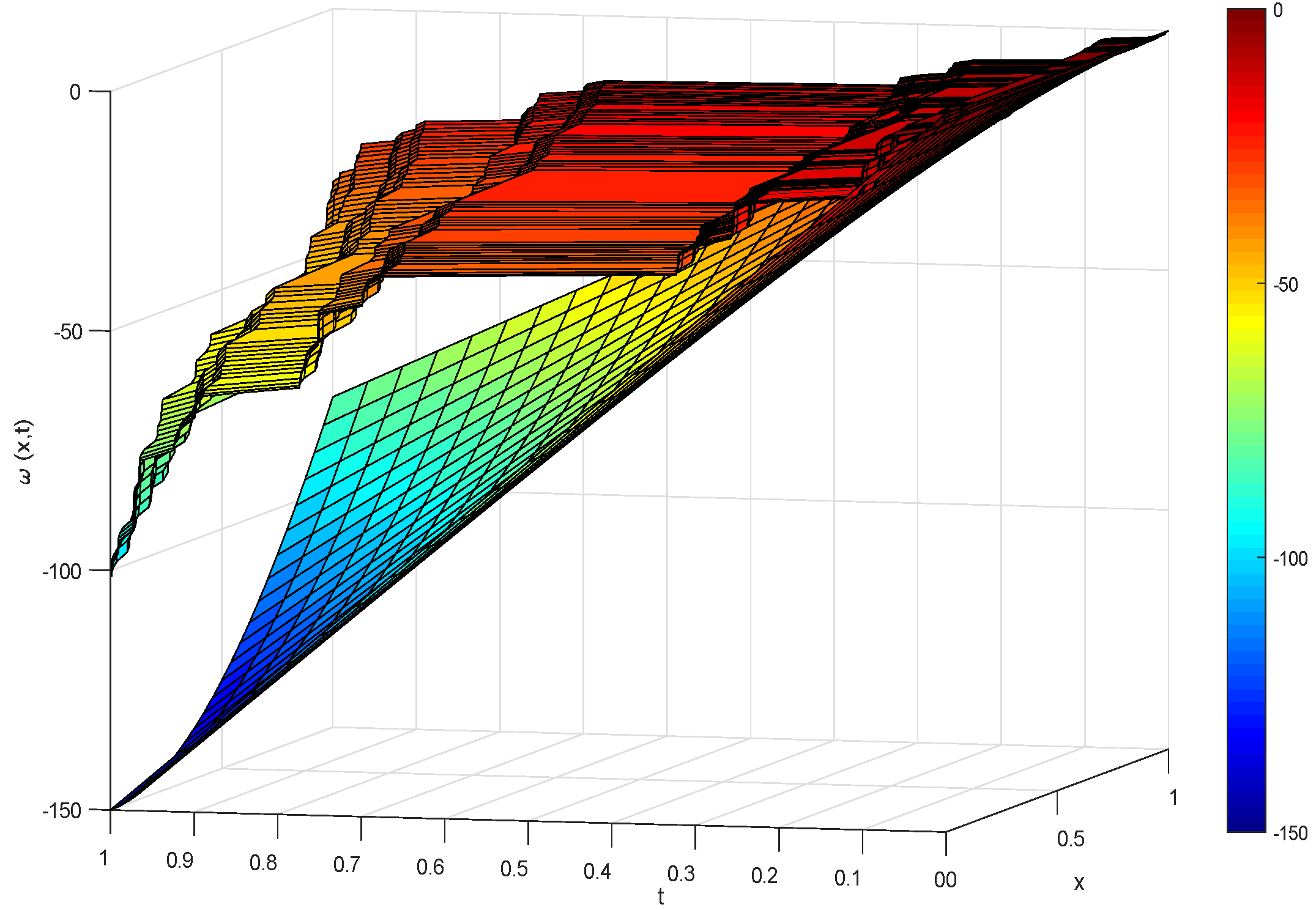
4. Solution of System of Equations

In this section, the solutions of coupled local fractional sine-Gordon equations are discussed.

We consider the following system of local fractional equations:

$$\left\{\begin{array}{c}\frac{{\mathsf{\partial }}^{2\epsilon }\psi }{\mathsf{\partial }{t}^{2\epsilon }}-\frac{{\mathsf{\partial }}^{2\epsilon }\psi }{\mathsf{\partial }{x}^{2\epsilon }}=-{\delta }^2{sin}_{\epsilon }{\left(\psi -\omega \right)}^{\epsilon },\hfill \\ \hfill \\ \frac{{\mathsf{\partial }}^{2\epsilon }\omega }{\mathsf{\partial }{t}^{2\epsilon }}-c^2\frac{{\mathsf{\partial }}^{2\epsilon }\omega }{\mathsf{\partial }{x}^{2\epsilon }}={sin}_{\epsilon }{\left(\psi -\omega \right)}^{\epsilon }.\hfill \end{array}\right.$$

(11)

In order to solve the coupled local part sine-Gordon equations, we can construct the following nondifferentiable homotopy:

$$\left\{\begin{array}{c}\left(1-{\rho }^{\epsilon }\right)\frac{{\mathsf{\partial }}^{2\epsilon }\psi }{\mathsf{\partial }{t}^{2\epsilon }}+{\rho }^{\epsilon }\left[\frac{{\mathsf{\partial }}^{2\epsilon }\psi }{\mathsf{\partial }{t}^{2\epsilon }}-\frac{{\mathsf{\partial }}^{2\epsilon }\psi }{\mathsf{\partial }{x}^{2\epsilon }}+{\delta }^2{sin}_{\epsilon }(\psi -\omega )\right]=0,\hfill \\ \hfill \\ \left(1-{\rho }^{\epsilon }\right)\frac{{\mathsf{\partial }}^{2\epsilon }\omega }{\mathsf{\partial }{t}^{2\epsilon }}+{\rho }^{\epsilon }\left[\frac{{\mathsf{\partial }}^{2\epsilon }\psi }{\mathsf{\partial }{t}^{2\epsilon }}-c^2\frac{{\mathsf{\partial }}^{2\epsilon }\omega }{\mathsf{\partial }{x}^{2\epsilon }}-{sin}_{\epsilon }(\psi -\omega )\right]=0.\hfill \end{array}\right.$$

(12)

Moreover,

$$\left\{\begin{array}{c}\psi =\sum _{j=0}^{\infty }{\rho }^{j\epsilon }{\psi }_j={\psi }_0+{\rho }^{\epsilon }{\psi }_1+{\rho }^{2\epsilon }{\psi }_2+\cdots ,\hfill \\ \hfill \\ \omega =\sum _{j=0}^{\infty }{\rho }^{j\epsilon }{\omega }_j={\omega }_0+{\rho }^{\epsilon }{\omega }_1+{\rho }^{2\epsilon }{\omega }_2+\cdots .\hfill \end{array}\right.$$

(13)

Submitting Equation (13) into Equation (12), we have

$$\left\{\begin{array}{c}\frac{{\mathsf{\partial }}^{2\epsilon }}{\mathsf{\partial }t}\left[\sum _{j=0}^{\infty }{\rho }^{j\epsilon }{\psi }_j(x,t)\right]-\frac{{\mathsf{\partial }}^{2\epsilon }{\psi }_0(x,t)}{\mathsf{\partial }{t}^{2\epsilon }}\hfill \\ ={\rho }^{\epsilon }\left\{\frac{{\mathsf{\partial }}^{2\epsilon }}{\mathsf{\partial }{x}^{2\epsilon }}\left[\sum _{j=0}^{\infty }{\rho }^{j\epsilon }{\psi }_j(x,t)\right]-{\delta }^2\left[\sum _{k=0}^{\infty }\frac{{(-1)}^k{(\psi -w)}^{2k+1}}{\mathsf{\Gamma }(1+(2k+1\left)\epsilon \right)}\right]-\frac{{\mathsf{\partial }}^{2\epsilon }{\psi }_0(x,t)}{\mathsf{\partial }{t}^{2\epsilon }}\right\},\hfill \\ \hfill \\ \frac{{\mathsf{\partial }}^{2\epsilon }}{\mathsf{\partial }{t}^{2\epsilon }}\left[\sum _{j=0}^{\infty }{\rho }^{j\epsilon }{\omega }_j(x,t)\right]-\frac{{\mathsf{\partial }}^{2\epsilon }{\omega }_0(x,t)}{\mathsf{\partial }{t}^{2\epsilon }}\hfill \\ ={\rho }^{\epsilon }\left\{c^2\frac{{\mathsf{\partial }}^{2\epsilon }}{\mathsf{\partial }{x}^{2\epsilon }}\left[\sum _{j=0}^{\infty }{\rho }^{j\epsilon }{\omega }_j(x,t)\right]+\left[\sum _{k=0}^{\infty }\frac{{(-1)}^k{(\psi -\omega )}^{2k+1}}{\mathsf{\Gamma }(1+(2k+1\left)\epsilon \right)}\right]-\frac{{\mathsf{\partial }}^{2\epsilon }{\omega }_0(x,t)}{\mathsf{\partial }{t}^{2\epsilon }}\right\}.\hfill \end{array}\right.$$

(14)

Taking $k=1,2,3$, then rearranging according to the power of $\rho$-terms, we obtain:

$${\rho }^{0\epsilon }:\left\{\begin{array}{c}\frac{{\mathsf{\partial }}^{2\epsilon }{\psi }_0(x,t)}{\mathsf{\partial }{t}^{2\epsilon }}-\frac{{\mathsf{\partial }}^{2\epsilon }{\psi }_0(x,t)}{\mathsf{\partial }{t}^{2\epsilon }}=0,{\psi }_0(x,t)=A{cos}_{\epsilon }\left(k{x}^{\epsilon }\right),\hfill \\ \hfill \\ \frac{{\mathsf{\partial }}^{2\epsilon }{\omega }_0(x,t)}{\mathsf{\partial }{t}^{2\epsilon }}-\frac{\mathsf{\partial }{\omega }_0(x,t)}{\mathsf{\partial }{t}^{2\epsilon }}=0,{\omega }_0(x,t)=0.\hfill \end{array}\right.$$

(15)

$${\rho }^{1\epsilon }:\left\{\begin{array}{c}\frac{{\mathsf{\partial }}^{2\epsilon }{\psi }_1}{\mathsf{\partial }{t}^{2\epsilon }}=\frac{{\mathsf{\partial }}^{2\epsilon }{\psi }_0}{\mathsf{\partial }{x}^{2\epsilon }}-{\delta }^2\frac{{\psi }_0-{\omega }_0}{\mathsf{\Gamma }(1+\epsilon )}+{\delta }^2\frac{{\psi }_0^3-3{\psi }_0^2{\omega }_0+3{\psi }_0{\omega }_0^3-{\omega }_0^3}{\mathsf{\Gamma }(1+3\epsilon )}\hfill \\ -{\delta }^2\frac{{\psi }_0^5-5{\psi }_0^4{\omega }_0+10{\psi }_0^3{\omega }_0^2-10{\psi }_0^2{\omega }_0^3+5{\psi }_0^2{\omega }_0^3+5{\psi }_0{\omega }_0^4-{\omega }_0^5}{\mathsf{\Gamma }(1+5\epsilon )}-\frac{{\mathsf{\partial }}^{2\epsilon }{\psi }_0}{\mathsf{\partial }{t}^{2\epsilon }},\hfill \\ \hfill \\ \frac{{\mathsf{\partial }}^{2\epsilon }{\omega }_1}{\mathsf{\partial }{t}^{2\epsilon }}=c^2\frac{{\mathsf{\partial }}^2{\omega }_0}{\mathsf{\partial }{x}^{2\epsilon }}+\frac{{\psi }_0-{\omega }_0}{\mathsf{\Gamma }(1+\epsilon )}-\frac{{\psi }_0^3-3{\psi }_0^2{\omega }_0+3{\psi }_0{\omega }_0^3-{\omega }_0^3}{\mathsf{\Gamma }(1+3\epsilon )}\hfill \\ +\frac{{\psi }_0^5-5{\psi }_0^4{\omega }_0+10{\psi }_0^3{\omega }_0^2-10{\psi }_0^2{\omega }_0^3+5{\psi }_0^2{\omega }_0^3+5{\psi }_0{\omega }_0^4-{\omega }_0^5}{\mathsf{\Gamma }(1+5\epsilon )}-\frac{{\mathsf{\partial }}^{2\epsilon }{\omega }_0}{\mathsf{\partial }{t}^{2\epsilon }}.\hfill \end{array}\right.$$

(16)

$${\rho }^{2\epsilon }:\left\{\begin{array}{c}\frac{{\mathsf{\partial }}^{2\epsilon }{\psi }_2}{\mathsf{\partial }{t}^{2\epsilon }}=\frac{{\mathsf{\partial }}^{2\epsilon }{\psi }_1}{\mathsf{\partial }{x}^{2\epsilon }}-{\delta }^2\left[\frac{{\psi }_1-{\omega }_1}{\mathsf{\Gamma }(1+\epsilon )}-\frac{1}{\mathsf{\Gamma }(1+3\epsilon )}\left(3{\psi }_0^2{\psi }_1-3{\psi }_0^2{\omega }_1-6{\psi }_0{\psi }_1{\omega }_0+6{\psi }_0{\omega }_0{\omega }_1+3{\psi }_1{\omega }_0^2-3{\omega }_0^2{\omega }_1\right)\right.\hfill \\ +\frac{1}{\mathsf{\Gamma }(1+5\epsilon )}\left(2{\psi }_0^3{\psi }_1+2{\psi }_0^4{\psi }_1-10{\psi }_0{\psi }_1{\omega }_0-5{\psi }_0^3{\psi }_1{\omega }_0-5{\psi }_0^4{\omega }_1+30{\psi }_0^2{\psi }_1{\omega }_0^2+20{\psi }_0^3{\omega }_0{\omega }_1\right.\hfill \\ \left.\left.-30{\psi }_0^2{\omega }_0^2{\omega }_1-20{\psi }_0{\psi }_1{\omega }_0^3+10{\psi }_0{\omega }_0{\omega }_1+5{\psi }_0{\omega }_0^3{\omega }_1+5{\psi }_1{\omega }_0^4-2{\omega }_0^3{\omega }_1-2{\omega }_0^4{\omega }_1\right)\right],\hfill \\ \hfill \\ \frac{{\mathsf{\partial }}^{2\epsilon }{\omega }_2}{\mathsf{\partial }{t}^{2\epsilon }}=c^2\frac{{\mathsf{\partial }}^{2\epsilon }{\omega }_1}{\mathsf{\partial }{x}^{2\epsilon }}+\frac{{\psi }_1-{\omega }_1}{\mathsf{\Gamma }(1+\epsilon )}-\frac{1}{\mathsf{\Gamma }(1+3\epsilon )}\left(3{\psi }_0^2{\psi }_1-3{\psi }_0^2{\omega }_1-6{\psi }_0{\psi }_1{\omega }_0+6{\psi }_0{\omega }_0{\omega }_1+3{\psi }_1{\omega }_0^2-3{\omega }_0^3{\omega }_1\right)\hfill \\ +\frac{1}{\mathsf{\Gamma }(1+5\epsilon )}\left(2{\psi }_0^3{\psi }_1+2{\psi }_0^4{\psi }_1-10{\psi }_0{\psi }_1{\omega }_0-5{\psi }_0^3{\psi }_1{\omega }_0-5{\psi }_0^4{\omega }_1+30{\psi }_0^2{\psi }_1{\omega }_0^2+20{\psi }_0^3{\omega }_0{\omega }_1\right.\hfill \\ \left.-30{\psi }_0^2{\omega }_0^2{\omega }_1-20{\psi }_0{\psi }_1{\omega }_0^3+10{\psi }_0{\omega }_0{\omega }_1+5{\psi }_0{\omega }_0^3{\omega }_1+5{\psi }_1{\omega }_0^4-2{\omega }_0^3{\omega }_1-2{\omega }_0^4{\omega }_1\right).\hfill \end{array}\right.$$

(17)

Solving Equations (15)–(17), we obtain:

$$\left\{\begin{array}{c}{\psi }_0(x,t)=Acos\left(k{x}^{\epsilon }\right),\hfill \\ \hfill \\ {\omega }_0(x,t)=0.\hfill \end{array}\right.$$

$$\left\{\begin{array}{cc}{\psi }_1(x,t)=\hfill & \frac{t^{2\epsilon }}{\mathsf{\Gamma }(1+2\epsilon )}\left[-A{k}^2{cos}_{\epsilon }\left(k{x}^{\epsilon }\right)-{\delta }^2\frac{1}{\mathsf{\Gamma }(1+\epsilon )}A{cos}_{\epsilon }\left(k{x}^{\epsilon }\right)\right.\hfill \\ & \left.+{\delta }^2\frac{1}{\mathsf{\Gamma }(1+3\epsilon )}{A}^3{cos}_{\epsilon }^3\left(k{x}^{\epsilon }\right)-{\delta }^2\frac{1}{\mathsf{\Gamma }(1+5\epsilon )}{A}^5{cos}_{\epsilon }^5\left(k{x}^{\epsilon }\right)\right],\hfill \\ \hfill \\ {\omega }_1(x,t)=\hfill & \frac{t^{2\epsilon }}{\mathsf{\Gamma }(1+2\epsilon )}\left[\frac{1}{\mathsf{\Gamma }(1+\epsilon )}A{cos}_{\epsilon }\left(k{x}^{\epsilon }\right)-\frac{1}{\mathsf{\Gamma }(1+3\epsilon )}{A}^3{cos}_{\epsilon }^3\left(k{x}^{\epsilon }\right)\right.\hfill \\ & \left.+\frac{1}{\mathsf{\Gamma }(1+5\epsilon )}{A}^5{cos}_{\epsilon }^5\left(k{x}^{\epsilon }\right)\right].\hfill \end{array}\right.$$

$$\begin{array}{cc}{\psi }_2(x,t)=\frac{t^{4\epsilon }}{\mathsf{\Gamma }(1+4\epsilon )}\hfill & \left\{A\left[k^2+2k^2\frac{{\delta }^2}{\mathsf{\Gamma }(1+\epsilon )}+\frac{{\delta }^4+{\delta }^2}{\mathsf{\Gamma }(1+\epsilon )\mathsf{\Gamma }(1+\epsilon )}+6A^2{k}^2\frac{{\delta }^2}{\mathsf{\Gamma }(1+3\epsilon )}\right]{cos}_{\epsilon }\left(k{x}^{\epsilon }\right)\right.\hfill \\ & -A^3\left[12k^2\frac{{\delta }^2}{\mathsf{\Gamma }(1+3\epsilon )}+20A^2{k}^2\frac{{\delta }^2}{\mathsf{\Gamma }(1+5\epsilon )}+4\frac{{\delta }^4+{\delta }^2}{\mathsf{\Gamma }(1+\epsilon )\mathsf{\Gamma }(1+3\epsilon )}\right]{cos}_{\epsilon }^3\left(k{x}^{\epsilon }\right)\hfill \\ & +A^5\left[27k^2\frac{{\delta }^2}{\mathsf{\Gamma }(1+5\epsilon )}+\frac{3{\delta }^4+6{\delta }^2}{\mathsf{\Gamma }(1+\epsilon )\mathsf{\Gamma }(1+5\epsilon )}+3\frac{{\delta }^4+{\delta }^2}{\mathsf{\Gamma }(1+3\epsilon )\mathsf{\Gamma }(1+3\epsilon )}\right]{cos}_{\epsilon }^5\left(k{x}^{\epsilon }\right)\hfill \\ & -A^7\left[\frac{5{\delta }^4+8{\delta }^2}{\mathsf{\Gamma }(1+3\epsilon )\mathsf{\Gamma }(1+5\epsilon )}\right]{cos}_{\epsilon }^7\left(k{x}^{\epsilon }\right)+A^9\left[\frac{2{\delta }^4+5{\delta }^2}{\mathsf{\Gamma }(1+5\epsilon )\mathsf{\Gamma }(1+5\epsilon )}\right]{cos}_{\epsilon }^9\left(k{x}^{\epsilon }\right)\hfill \\ & +A^4\left[2k^2\frac{{\delta }^2}{\mathsf{\Gamma }(1+5\epsilon )}+2\frac{{\delta }^4}{\mathsf{\Gamma }(1+\epsilon )\mathsf{\Gamma }(1+5\epsilon )}\right]{cos}_{\epsilon }^4\left(k{x}^{\epsilon }\right)\hfill \\ & \left.-A{}^6\left[2\frac{{\delta }^4}{\mathsf{\Gamma }(1+3\epsilon )\mathsf{\Gamma }(1+5\epsilon )}\right]{cos}_{\epsilon }^6\left(k{x}^{\epsilon }\right)+A^8\left[2\frac{{\delta }^4}{\mathsf{\Gamma }(1+5\epsilon )\mathsf{\Gamma }(1+5\epsilon )}\right]{cos}_{\epsilon }^8\left(k{x}^{\epsilon }\right)\right\},\hfill \end{array}$$

$$\begin{array}{cc}{\omega }_2(x,t)=\frac{t^{4\epsilon }}{\mathsf{\Gamma }(1+4\epsilon )}\hfill & \left\{-A\left[k^2\frac{c^2+1}{\mathsf{\Gamma }(1+\epsilon )}+\frac{{\delta }^2+1}{\mathsf{\Gamma }(1+\epsilon )\mathsf{\Gamma }(1+\epsilon )}+6A^2{k}^2\frac{c^2}{\mathsf{\Gamma }(1+3\epsilon )}\right]{cos}_{\epsilon }\left(k{x}^{\epsilon }\right)\right.\hfill \\ & +A^3\left[12k^2\frac{c^2}{\mathsf{\Gamma }(1+3\epsilon )}+20A^2{k}^2\frac{c^2}{\mathsf{\Gamma }(1+5\epsilon )}+4\frac{{\delta }^2+1}{\mathsf{\Gamma }(1+\epsilon )\mathsf{\Gamma }(1+3\epsilon )}\right]{cos}_{\epsilon }^3\left(k{x}^{\epsilon }\right)\hfill \\ & -A^5\left[27k^2\frac{c^2}{\mathsf{\Gamma }(1+5\epsilon )}+\frac{3{\delta }^2+6}{\mathsf{\Gamma }(1+\epsilon )\mathsf{\Gamma }(1+5\epsilon )}+3\frac{{\delta }^2+1}{\mathsf{\Gamma }(1+3\epsilon )\mathsf{\Gamma }(1+3\epsilon )}\right]{cos}_{\epsilon }^5\left(k{x}^{\epsilon }\right)\hfill \\ & +A^7\left[\frac{5{\delta }^2+8}{\mathsf{\Gamma }(1+3\epsilon )\mathsf{\Gamma }(1+5\epsilon )}\right]{cos}_{\epsilon }^7\left(k{x}^{\epsilon }\right)-A^9\left[\frac{2{\delta }^2+5}{\mathsf{\Gamma }(1+5\epsilon )\mathsf{\Gamma }(1+5\epsilon )}\right]{cos}_{\epsilon }^9\left(k{x}^{\epsilon }\right)\hfill \\ & -A^4\left[2k^2\frac{1}{\mathsf{\Gamma }(1+5\epsilon )}+2\frac{{\delta }^2}{\mathsf{\Gamma }(1+\epsilon )\mathsf{\Gamma }(1+5\epsilon )}\right]{cos}_{\epsilon }^4\left(k{x}^{\epsilon }\right)\hfill \\ & \left.+A^6\left[2\frac{{\delta }^2}{\mathsf{\Gamma }(1+3\epsilon )\mathsf{\Gamma }(1+5\epsilon )}\right]{cos}_{\epsilon }^6\left(k{x}^{\epsilon }\right)-A^8\left[2\frac{{\delta }^2}{\mathsf{\Gamma }(1+5\epsilon )\mathsf{\Gamma }(1+5\epsilon )}\right]{cos}_{\epsilon }^8\left(k{x}^{\epsilon }\right)\right\}.\hfill \end{array}$$

When $\rho \to 1$, the solutions of the coupled local fractional sine-Gordon equations are

$$\left\{\begin{array}{c}\psi (x,t)={\psi }_0(x,t)+{\psi }_1(x,t)+{\psi }_2(x,t),\hfill \\ \hfill \\ \omega (x,t)={\omega }_0(x,t)+{\omega }_1(x,t)+{\omega }_2(x,t).\hfill \end{array}\right.$$

(18)

When the fractal dimension is $\epsilon =ln2/ln3$, the corresponding diagrams of $\psi (x,t)$ and $\omega (x,t)$ are as shown in Figure 1 and Figure 2.

The time-dependent behavior of $\psi (x,t)$ and $\omega (x,t)$ obtained from the theory of the local number order homotopy perturbation method is shown in Figure 3. We show the elastic interaction between two solitons. It can be seen that both solitons maintain their initial velocity and shape after interaction. In Figure 4, we compare the local motion diagram of the sine-Gordon equation with integer order and fractal dimension $\epsilon =ln2/ln3$. Compared with the general homotopy perturbation method, the behavior graph obtained by this method is more realistic.

5. Conclusions

In this paper, we obtain the exact solution of a coupled local fractional sinusoidal Gordon equation by using the LFHP method, and show the special function graphs defined on the Cantor set when the fractal dimension is $\epsilon =ln2/ln3$. The results show that the technique is effective in solving nonlinear partial order equations. The LFHP method solves many nonlinear problems in science and engineering. We consider that the LFHP method can theoretically solve the ac-driven sine-Gordon equation [29]. We will study it in future work. With the help of MATLAB and other mathematical software, this method provides a powerful mathematical tool for more complex nonlinear systems. In a word, the LFHP method provides highly accurate fractal solutions for nonlinear problems.

References

1. Charpentier, I. On Higher-order Differentiation in Nonlinear Mechanics. Optim. Methods Softw. 2012, 27, 221–232. [Google Scholar] [CrossRef]
2. Viana, R.L.; Silva, E.; Kroetz, T.; Caldas, I.T.; Roberto, M.; Sanjuan, A.F. Fractal Structures in Nonlinear Plasma Physics. Philos. Trans. R. Soc. A 2011, 369, 371–395. [Google Scholar] [CrossRef] [PubMed] [Green Version]
3. Kalashnikov, A.S. The Propagation of Disturbances in Problem of Nonlinear Heat Conduction with Absorption. Comput. Math. Math. Phys. 1974, 14, 70–85. [Google Scholar] [CrossRef]
4. Chowdhury, A.R.; Pal, S.K. N-fold Backlund Transformation for Deformed Nonlinear Schrödinger Equation. Int. J. Theor. Phys. 1997, 36, 1021–1031. [Google Scholar] [CrossRef]
5. Liu, W.J.; Tian, B.; Zhang, H.Q.; Li, L.L.; Xue, Y.S. Soliton Interaction in the Higher-order Nonlinear Schrodinger equation Investigated with Hirota’s Bilinear Method. Phys. Rev. E 2008, 77, 066605. [Google Scholar] [CrossRef]
6. Wazwaz, A.M. A Sine-cosine Method for Handling Nonlinear Wave Equations. Math. Comput. Model. 2004, 40, 499–508. [Google Scholar] [CrossRef]
7. Ray, S.S.; Bera, R.K. An Approximate Solution of a Nonlinear Fractional Differential Equation by Adomian Decomposition Method. Appli. Math. Comp. 2005, 167, 561–571. [Google Scholar]
8. Askari, H.; Zhang, D.; Esmailzadeh, E. Periodic Solutions for Nonlinear Oscillations of Nanowires Using Variational Iteration Method. In Proceedings of the 2013 13th IEEE International Conference on Nanotechnology (IEEE-NANO 2013), Beijing, China, 5–8 August 2013. [Google Scholar]
9. Wu, X.H.; He, J.H. EXP-function Method and its Application to Nonlinear Equations. Chaos Solitons Fractals 2008, 38, 903–910. [Google Scholar]
10. Rajabi, A.; Ganji, D.D.; Taherian, H. Application of Homotopy Perturbation Method in Nonlinear Heat Conduction and Convection Equations. Phys. Lett. 2007, 360, 570–573. [Google Scholar] [CrossRef]
11. Asllanaj, F.; Jeandel, G.; Roche, J.R. Numerical Solution of Radiative Transfer Equation Coupled with Nonlinear Heat Conduction Equation. Int. J. Numer. Methods Heat Fluid Flow 2015, 11, 449–473. [Google Scholar] [CrossRef]
12. He, J.H. Application of Homotopy Perturbation Method to Nonlinear Wave Equations. Chaos Solitons Fractals 2005, 26, 695–700. [Google Scholar] [CrossRef]
13. Ganji, D.D.; Sadighi, A.; Ganjavi, B. Traveling Wave Solutions of the Sine-gordon and the Coupled Sine-gordon Equations Using the Homotopy-perturbation Method. Sci. Iran. 2009, 16, 189–195. [Google Scholar]
14. Mustafa Inc. He’s Homotopy Perturbation Method for Solving Korteweg-de Vries Burgers Equation with Initial Condition. Numer. Methods Partial. Differ. Equ. 2010, 26, 1224–1235. [Google Scholar]
15. Ganji, D.D. The Application of He’s Homotopy Perturbation Method to Nonlinear Equations Arising in Heat Transfer-Science Direct. Phys. Lett. A 2006, 355, 337–341. [Google Scholar] [CrossRef]
16. Ganji, D.D.; Sadighi, A. Application of He’s Homotopy-perturbation Method to Nonlinear Coupled Systems of Reaction-diffusion Equations. Int. J. Nonlinear Sci. Num. Simul. 2006, 7, 411–418. [Google Scholar] [CrossRef]
17. Yang, X.J. Advanced Local Fractional Calculus and Its Applications; Orld Science: New York, NY, USA, 2012. [Google Scholar]
18. Yang, X.J.; Srivastava, H.M.; Cattani, C. Local Fractional Homotopy Perturbation Method for Solving Fractal Partial Differential Equation Arising in Mathematical Physics. Rom. Rep. Phys. 2015, 67, 752–761. [Google Scholar]
19. Zhang, Y.; Carlo, C. and Yang, X.J. Local Fractional Homotopy Perturbation Method for Solving Non-Homogeneous Heat Conduction Equations in Fractal Domains. Entropy 2015, 17, 6753–6764. [Google Scholar] [CrossRef] [Green Version]
20. Braun, O.M.; Kivshar, Y.S. Nonlinear Dynamics of the Frenkel-Kontorova Model with Impurities. Phys. Rev. B Condens Matter 1998, 306, 1060–1073. [Google Scholar] [CrossRef]
21. Saha, S.; Ray. A Numerical Solution of the Coupled Sine-Gordon Equation Using the Modified Decomposition Method. Appl. Math. Comput. 2006, 175, 1046–1054. [Google Scholar]
22. Hosseini, K.; Mayeli, P.; Kumar, D. New exact solutions of the coupled sine-Gordon equations in nonlinear optics using the modified Kudryashov method. J. Mod. Opt. 2017, 65, 361–364. [Google Scholar] [CrossRef]
23. Salas, A.H. Exact Solutions of Coupled Sine-Gordon Equations. Nonlinear Anal.-Real 2010, 11, 3930–3935. [Google Scholar] [CrossRef]
24. Zhao, Y.M.; Liu, H.H.; Yang, Y.J. Exact Solutions for the Coupled Sine-Gordon Equations by a New Hyperbolic Auxiliary Function Method. Appl. Math. Sci. 2011, 5, 1621–1629. [Google Scholar]
25. Yang, X.J.; Machado, J.A.T.; Hristov, J. Nonlinear Dynamics for Local Fractional Burgers’ equation Arising in Fractal Flow. Nonlinear Dyn. 2016, 84, 3–7. [Google Scholar] [CrossRef] [Green Version]
26. Ghanbari, B. On Novel Nondifferentiable Exact Solutions to Local Fractional Gardner’s Equation Using an Effective Technique. Math. Method Appl. Sci. 2021, 44, 4673–4685. [Google Scholar] [CrossRef]
27. Yang, X.J.; Machado, J.T.; Baleanu, D.; Cattani, C. On Exact Traveling-wave Solutions for Local Fractional Korteweg-de Vries Equation. Chaos 2016, 26, 110–118. [Google Scholar] [CrossRef]
28. Yang, X.J. Local Fractional Integral Transforms and Their Applications; Academic Press: Cambridge, MA, USA, 1995. [Google Scholar]
29. Quintero, R.N.; Sánchez, A. Ac driven sine-Gordon solitons: Dynamics and stability. Eur. Phys. J. B 1998, 6, 133–142. [Google Scholar] [CrossRef] [Green Version]
Figure 1. In the case of ψ ( x , t ) solution in the local fractional sine-Gordon equations, by choosing A = 1 , k = 1 , c = 1 , δ = 1 . (a) 0 ≤ t ≤ 1; (b) −1 ≤ t ≤ 1.
Fractalfract 06 00404 g001
Figure 2. In the case of ω ( x , t ) solution in the local fractional sine-Gordon equations, by choosing A = 1 , k = 1 , c = 1 , δ = 1 . (a) 0 ≤ t ≤ 1; (b) −1 ≤ t ≤ 1.
Fractalfract 06 00404 g002
Figure 3. In the case of local fractional sine-Gordon equations, by choosing parameters A = 1 , k = 1 , c = 1 , δ = 1 .
Fractalfract 06 00404 g003
Figure 4. Comparison of integer order ε = 1 and fractional dimension ε = l n 2 / l n 3 .
Fractalfract 06 00404 g004
Publisher’s Note: MDPI stays neutral with regard to jurisdictional claims in published maps and institutional affiliations.