Second Derivative Block Hybrid Methods for the Numerical Integration of Differential Systems

Abstract

The second derivative block hybrid method for the continuous integration of differential systems within the interval of integration was derived. The second derivative block hybrid method maintained the stability properties of the Runge–Kutta methods suitable for solving stiff differential systems. The lack of such stability properties makes the continuous solution not reliable, especially in solving large stiff differential systems. We derive these methods by using one intermediate off-grid point in between the familiar grid points for continuous solution within the interval of integration. The new family had a high accuracy, non-overlapping piecewise continuous solution with very low error constants and converged under the suitable conditions of stability and consistency. The results of computational experiments are presented to demonstrate the efficiency and usefulness of the methods, which also indicate that the block hybrid methods are competitive with some strong stability stiff integrators.

1. Introduction

The system whose numerical approximation is sought is written in the form

$$\{\begin{array}{l}\frac{dy}{dx}=f(x,y),\hspace{1em}\hspace{1em}(a\le x\le b),\\ y(x_0)=y_0\hspace{0.17em}\hspace{0.17em}.\end{array}$$

(1)

In Equation (1), $y:[a,b]\to R^m$ and $f:[a,b]\times R^m\to R^m$ are differentiable. To obtain accurate integration methods, which combine, to some extent, the advantages of the Runge–Kutta methods (RKMs) and linear multistep methods (LMMs), the use of the multistep collocation technique has been proposed by many authors, for example, Onumanyi et al. [1], Chollom and Jackiewicz [2], Chollom and Onumanyi [3], and Jator [4]. In this work, methods were designed for finding a continuous approximate solution of the system in Equation (1), where y(x) belongs to C¹([a, b], R^m) and the set of points defined as

$$\mathsf{\Omega }:a=x_0<x_1<\cdots <x_{n+1}=b,$$

so that

$$x_n:x_n=x_0+nh, n=0,1,\cdots ,N-1,h=x_{n+1}-x_n \mathrm{and} N=(b-a)/h.$$

The h in this paper, for simplicity, is a constant and N is a positive integer. Some of the methods derived for Equation (1) were, in fact, to evaluate the solution only at the first derivative of Equation (1). Long before our consideration of introducing the off-step points, Gragg and Stetter [5], Butcher [6,7], and Gear [8] had already considered introducing some off-step points and referred to them as generalized multistep predictor–corrector methods, a modified multistep method, and hybrid methods, respectively. Similarly, the introduction of the second derivative terms had already been considered by many authors. For example, earlier, Urabe [9] worked on a second derivative method with $y^{″}(x)=g(x,y)$ to obtain a starting method for the single-step integrator in the paper. In [10], Mitsui changed slightly Urabe’s PC pair to improve the performance of the method. To unify and extend this result after some years, Cash [11] generalized the PC pair of Urabe’s type of method. Gupta, in [12], derived and implemented second-derivative methods. Shaintani [13,14] suggested some integration algorithms very similar to RKMs, with $y^{\prime }(x)=f(x,y)$ and $y^{″}(x)=g(x,y)$. In [15], the author constructed $(p,q)$-stage RKMs, which exhibit $y^{″}(x)=g(x,y)$ evaluation. Chan and Tsai [16] considered explicit two-derivative RKMs, which are cheaper to calculate with fewer function evaluations than the standard RKMs. Recently, many authors have worked on methods to obtain better approximate solutions to differential equations or on stability properties to improve the accuracy and efficiency of solution of differential equations (see, for example, [17,18,19,20,21,22,23,24]).

In this article, we extend the work of Yakubu et al. [25] to derive block-hybrid methods that show a high order of accuracy with very low error constants and large regions of absolute stability and converge rapidly to the required solution. We should also point out that the effectiveness of this class of methods for the treatment of stiff systems is shown on the basis of their attractive properties and the efficient technique to deal with a large system of a stiff initial value problem of ordinary differential equations.

Definition 1

([26]). Let $Y_m$ and $F_m$ be vectors given by

$$Y_m={(y_n,y_{n+1},\dots ,y_{n+r-1})}^T,$$

$$F_m={(f_n,f_{n+1},\dots ,f_{n+r-1})}^T.$$

Then the k-block method is of the form

$$Y_m={\displaystyle \sum _{i=1}^k{A}_i{Y}_{m-i}}+{\displaystyle \sum _{i=0}^k{B}_i}{F}_{m-i}.$$

(2)

If r = 1, then the above equation in Equation (2) is just the classical k-step method. When B₀ = 0, Equation (2) is explicit; otherwise, it is implicit.

The below diagram depicts the idea of the new methods.

In Figure 1, [a, b] is divided into a series of equal lengths of a block of six points with size or length h. The approximate solutions $\{y_{n+u},y_{n+1},y_{n+v},y_{n+2},y_{n+w},y_{n+3}\}$ are computed simultaneously in the block at the points $\{x_{n+u},x_{n+1},x_{n+v},x_{n+2},x_{n+w},x_{n+3}\}$ in the kth block. Since the methods are self-starting, we do not need predictors to start the block methods.

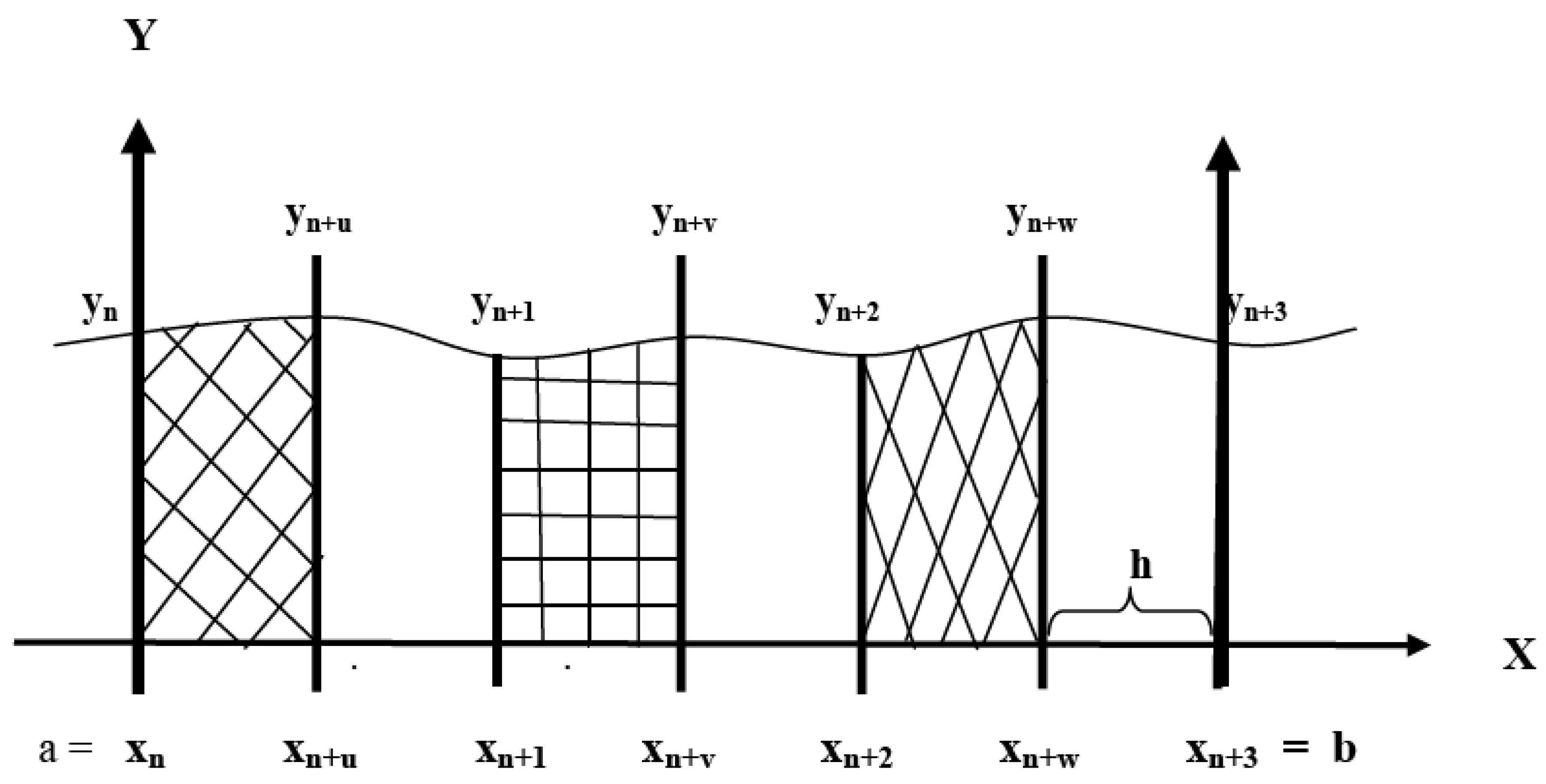
2. The Block Hybrid Methods

The block hybrid methods in this segment are based on the polynomial of the form

$$y(x)={\alpha }_0+{\alpha }_{1}x+{\alpha }_2{x}^2+\cdots +{\alpha }_{p-1}{x}^{p-1}={\displaystyle \sum _{i=0}^{p-1}{\alpha }_i}{x}^i$$

(3)

and are referred to as interpolation polynomials, which is twice continuously differentiable. The $y(x)$ is interpolated at $\left\{x_{n+j}\right\}$, and $y^{\prime }(x)$ and $y^{″}(x)$ are collocated at $\left\{c_{n+j}\right\}$ to obtain the system,

$$y(x_{n+j})=y(x_n+jh),\hspace{1em}\hspace{1em}\hspace{1em}\hspace{1em}\hspace{1em}j\in \left\{0,1,2,\dots ,r-1\right\},$$

(4)

$$y^{\prime }(c_{n+j})=f_{n+j}=f(x_n+jh,y(x_n+jh)),\hspace{1em}\hspace{1em}j=0,1,2,\dots ,s-1,$$

(5)

$$y^{″}(c_{n+j})=g_{n+j}=f_x+f_y{y}^{\prime }=f_x+f{f}_y,\hspace{1em}\hspace{1em}j=0,1,2,\dots ,t-1.$$

(6)

Following Yakubu et al. [25], we put Equations (4)–(6) as:

$$V\alpha =y$$

(7)

to have

$$V\hspace{0.17em}\hspace{0.17em}\hspace{0.17em}=\hspace{0.17em}\hspace{0.17em}\hspace{0.17em}\left(\begin{array}{lllllll}1& \hspace{1em}{x}_n& x_n^2& x_n^3& x_n^4& \cdots & x_n^{p-1}\\ ⋮& \hspace{1em}⋮& ⋮& ⋮& ⋮& \ddots & ⋮\\ 1& \hspace{1em}{x}_{n+r-1}& x_{n+r-1}^2& x_{n+r-1}^3& x_{n+r-1}^4& \cdots & x_{n+r-1}^{p-1}\\ 0& \hspace{1em}1& 2x_n& 3x_n^2& 4x_n^3& \cdots & D^{\prime }{x}_n^{p-2}\\ ⋮& \hspace{1em}⋮& ⋮& ⋮& ⋮& \ddots & ⋮\\ 0& \hspace{1em}1& 2x_{n+s-1}& 3x_{n+s-1}^2& 4x_{n+s-1}^3& \cdots & D^{\prime }{x}_{n+s-1}^{p-2}\\ 0& \hspace{1em}0& 2& 6x_n& 12x_n^2& \cdots & D^{″}{x}_n^{p-3}\\ ⋮& \hspace{1em}⋮& ⋮& ⋮& ⋮& \ddots & ⋮\\ 0& \hspace{1em}0& 2\cdots & 6x_{n+t-1}& 12x_{n+t-1}^2& \cdots & D^{″}\hspace{0.17em}{x}_{n+t-1}^{p-3}\end{array}\right)$$

(8)

$$\alpha ={({\alpha }_0,{\alpha }_1,{\alpha }_2,\cdots ,{\alpha }_{p-1})}^T, y={(y_n,\cdots ,y_{n+r-1},f_n,\cdots ,f_{n+s-1},\hspace{0.17em}{g}_n,\hspace{0.17em}\cdots ,g_{n+t-1})}^T.$$

The $D^{\prime }=(p-1)$ and $D^{″}=(p-1)(p-2)$ are first and second derivatives. From Equation (7), we have

$$\alpha =Uy, \mathrm{where} U=V^{-1}$$

(9)

which is rearranged to have

$$y(x)={\displaystyle \sum _{j=0}^{r-1}{\alpha }_j}(x)y_{n+j}+h{\displaystyle \sum _{j=0}^{s-1}{\beta }_j(x)f_{n+j}+}{h}^2{\displaystyle \sum _{j=0}^{t-1}{\gamma }_j(x)g_{n+j}},$$

(10)

where

$${\alpha }_j(x)={\displaystyle \sum _{i=0}^{p-1}{\alpha }_{j,\hspace{0.17em}i+1}{x}^i,}\hspace{1em}\hspace{1em}\hspace{1em}j=0,\hspace{0.17em}\hspace{0.17em}1,\hspace{0.17em}\hspace{0.17em}2,\hspace{0.17em}\hspace{0.17em}\dots ,\hspace{0.17em}r-1,$$

(11a)

$$h{\beta }_j(x)=h{\displaystyle \sum _{i=0}^{p-1}{\beta }_{j,\hspace{0.17em}i+1}{x}^i},\hspace{1em}\hspace{1em}j=0,\hspace{0.17em}\hspace{0.17em}1,\hspace{0.17em}\hspace{0.17em}2,\hspace{0.17em}\hspace{0.17em}\dots ,\hspace{0.17em}s-1,$$

(11b)

$$h^2{\gamma }_j(x)=h^2{\displaystyle \sum _{i=0}^{p-1}{\gamma }_{j,\hspace{0.17em}i+1}{x}^i},\hspace{1em}j=0,\hspace{0.17em}\hspace{0.17em}1,\hspace{0.17em}\hspace{0.17em}2,\hspace{0.17em}\hspace{0.17em}\dots ,\hspace{0.17em}t-1.$$

(11c)

In fact, the coefficients in Equation (11) can be calculated from the inverse of the matrix U, as in Equation (9), or written as

$$U=V^{-1}.$$

(12)

Insert Equation (11) into Equation (10) (see Yakubu et al. [25,27]) to have

$$y(x)={\displaystyle \sum _{j=0}^{r-1}{\displaystyle \sum _{i=0}^{r+s+t-1}{\alpha }_{i+1,j}}}{y}_{n+j}{P}_i(x)+h{\displaystyle \sum _{j=0}^{s-1}{\displaystyle \sum _{i=0}^{r+s+t-1}{\beta }_{i+1,j}{f}_{n+j}}{P}_i(x)+}{h}^2{\displaystyle \sum _{j=0}^{t-1}{\displaystyle \sum _{i=0}^{r+s+t-1}{\gamma }_{i+1,j}}{g}_{n+j}{P}_i(x)}$$

which is factorized to obtain

$$\begin{array}{l}y(x)={\displaystyle \sum _{i=0}^{r+s+t-1}\left\{{\displaystyle \sum _{j=0}^{r-1}{\alpha }_{i+1,j}}{y}_{n+j}+h{\displaystyle \sum _{j=0}^{s-1}{\beta }_{i+1,j}{f}_{n+j}+}{h}^2{\displaystyle \sum _{j=0}^{t-1}{\gamma }_{i+1,j}{g}_{n+j}}\right\}{P}_i(x)}\\ \hspace{1em}={\displaystyle \sum _{i=0}^{r+s+t-1}{\phi }_i}{P}_i(x)\end{array}$$

(13)

where

$${\varphi }_i={\displaystyle \sum _{j=0}^{r-1}{\alpha }_{i+1,j}}{y}_{n+j}+h{\displaystyle \sum _{j=0}^{s-1}{\beta }_{i+1,j}{f}_{n+j}+}{h}^2{\displaystyle \sum _{j=0}^{t-1}{\gamma }_{i+1,j}{g}_{n+j}}.$$

Then Equation (13) becomes

$$y(x)=\{{\displaystyle \sum _{j=0}^{r-1}{\alpha }_{j,1}}{y}_{n+j}+h{\displaystyle \sum _{j=0}^{s-1}{\beta }_{j,1}{f}_{n+j}+}{h}^2{\displaystyle \sum _{j=0}^{t-1}{\gamma }_{j,1}{g}_{n+j}},$$

$$\begin{array}{l}{\displaystyle \sum _{j=0}^{r-1}{\alpha }_{j,2}}{y}_{n+j}+h{\displaystyle \sum _{j=0}^{s-1}{\beta }_{j,2}{f}_{n+j}+}{h}^2{\displaystyle \sum _{j=0}^{t-1}{\gamma }_{j,2}{g}_{n+j,}}\\ \hspace{0.17em}\hspace{0.17em}⋮\hspace{0.17em}\hspace{0.17em}\hspace{0.17em}\hspace{0.17em}\hspace{0.17em}\hspace{0.17em}\hspace{0.17em}\hspace{0.17em}\hspace{0.17em}\hspace{0.17em}\hspace{0.17em}\hspace{0.17em}\hspace{0.17em}\hspace{0.17em}\hspace{0.17em}\hspace{0.17em}\hspace{0.17em}\hspace{0.17em}⋮\hspace{0.17em}\hspace{0.17em}\hspace{0.17em}\hspace{0.17em}\hspace{0.17em}\hspace{0.17em}\hspace{0.17em}\hspace{0.17em}\hspace{0.17em}\hspace{0.17em}\hspace{0.17em}\hspace{0.17em}\hspace{0.17em}\hspace{0.17em}\hspace{0.17em}\hspace{0.17em}\hspace{0.17em}\hspace{0.17em}\hspace{0.17em}\hspace{0.17em}\hspace{0.17em}⋮\hspace{0.17em}\hspace{0.17em}\hspace{0.17em}\end{array}$$

$${\displaystyle \sum _{j=0}^{r-1}{\alpha }_{j,r+s+t-1}}{y}_{n+j}+h{\displaystyle \sum _{j=0}^{s-1}{\beta }_{j,r+s+t-1}{f}_{n+j}+}{h}^2{\displaystyle \sum _{j=0}^{t-1}{\gamma }_{j,r+s+t-1}{g}_{n+j}}\}{\left(1,x,x^2,\cdots ,x^{r+s+t-1}\right)}^T\hspace{0.17em}.$$

(14)

Expanding Equation (14) fully, we obtain

$$y(x)={(y_n,\cdots ,y_{n+r-1},f_n,\cdots ,f_{n+s-1},g_n,\cdots ,g_{n+t-1})}^T{U}^T{(1,x,\cdots ,x^{r+s+t-1})}^T.$$

(15)

The T in Equation (15) denotes the transpose of.

3. Specification of the Multistep Block Hybrid Methods

3.1. Block Hybrid Method of Seventh Order

In this segment, we use the multistep approach for the construction of the new block hybrid method with symmetric points of order seven. We introduce three off-step points, $u=\frac{1}{2}$, $v=\frac{3}{2}$, and $w=\frac{5}{2}$, and $\eta =(x-x_n)$ for the construction of the continuous scheme. These points are carefully chosen to guarantee the convergence of the method, as pointed out by [28,29,30]. From Equation (10), putting $r=1$ and $s=7$ gives the block hybrid method of the form

$$y(x)={\alpha }_0(x)y_n+h{\displaystyle \sum _{j=0}^6{\beta }_j}(x)f_{n+j}.$$

(16)

Simplifying Equation (16), the interpolation and collocation polynomial in Equation (10) reduces to the proposed continuous scheme of the form in Equation (15), as follows:

$$y(x)={\alpha }_0(x)y_n+h\left[{\beta }_0(x)f_n+{\beta }_1(x)f_{n+u}+{\beta }_2(x)f_{n+1}+{\beta }_3(x)f_{n+v}+{\beta }_4(x)f_{n+2}+{\beta }_5(x)f_{n+w}+{\beta }_6(x)f_{n+3}\right]$$

(17)

where

$${\alpha }_0(x)=1,$$

$${\beta }_0(x)=\left[\frac{96{\eta }^7-1176h{\eta }^6+5880h^2{\eta }^5-\mathrm{15,435}{h}^3{\eta }^4+\mathrm{22,736}{h}^4{\eta }^3-\mathrm{18,522}{h}^5{\eta }^2+7560h^6\eta }{7560h^6}\right],$$

$${\beta }_1(x)=\left[\frac{-24{\eta }^7+280h{\eta }^6-1302h^2{\eta }^5+3045h^3{\eta }^4-3654h^4{\eta }^3+1890h^5{\eta }^2}{315h^6}\right],$$

$${\beta }_2(x)=\left[\frac{480{\eta }^7-5320h{\eta }^6+\mathrm{23,016}{h}^2{\eta }^5-\mathrm{48,405}{h}^3{\eta }^4+\mathrm{49,140}{h}^4{\eta }^3-\mathrm{18,900}{h}^5{\eta }^2}{2520h^6}\right]\hspace{0.17em},$$

$${\beta }_3(x)=\left[\frac{-240{\eta }^7+2520h{\eta }^6-\mathrm{10,164}{h}^2{\eta }^5+\mathrm{19,530}{h}^3{\eta }^4-\mathrm{17,780}{h}^4{\eta }^3+6300h^5{\eta }^2}{945h^6}\right]\hspace{0.17em},$$

$${\beta }_4(x)=\left[\frac{480{\eta }^7-4760h{\eta }^6+\mathrm{17,976}{h}^2{\eta }^5-\mathrm{32,235}{h}^3{\eta }^4+\mathrm{27,720}{h}^4{\eta }^3-9450h^5{\eta }^2}{2520h^6}\right]\hspace{0.17em},$$

$${\beta }_5(x)=\left[\frac{-24{\eta }^7+224h{\eta }^6-798h^2{\eta }^5+1365h^3{\eta }^4-1134h^4{\eta }^3+378h^5{\eta }^2}{315h^6}\right]\hspace{0.17em},$$

$${\beta }_6(x)=\left[\frac{96{\eta }^7-840h{\eta }^6+2856h^2{\eta }^5-4725h^3{\eta }^4+3836h^4{\eta }^3-1260h^5{\eta }^2}{7560h^6}\right],$$

Evaluate Equation (17) at $x_{n+u}$, $x_{n+1}$$x_{n+v}$, $x_{n+2}$, $x_{n+w}$, and $x_{n+3}$ to obtain the method:

$$y_{n+u}=y_n+\frac{h}{\mathrm{120,960}}\left[\mathrm{19,087}{f}_n+\mathrm{65,112}{f}_{n+u}-\mathrm{46,461}{f}_{n+1}+\mathrm{37,504}{f}_{n+v}-\mathrm{20,211}{f}_{n+2}+6312f_{n+w}-863f_{n+3}\right]$$

(18)

$$y_{n+1}=y_n+\frac{h}{7560}\left[1139f_n+5640f_{n+u}+33f_{n+1}+1328f_{n+v}-807f_{n+2}+264f_{n+w}-37f_{n+3}\right]$$

$$y_{n+v}=y_n+\frac{h}{4480}\left[685f_n+3240f_{n+u}+1161f_{n+1}+2176f_{n+v}-729f_{n+2}+216f_{n+w}-29f_{n+3}\right]$$

$$y_{n+2}=y_n+\frac{h}{945}\left[143f_n+696f_{n+u}+192f_{n+1}+752f_{n+v}+87f_{n+2}+24f_{n+w}-4f_{n+3}\right]$$

$$y_{n+w}=y_n+\frac{h}{\mathrm{24,192}}\left[3715f_n+\mathrm{17,400}{f}_{n+u}+6375f_{n+1}+\mathrm{16,000}{f}_{n+v}+\mathrm{11,625}{f}_{n+2}+5640f_{n+w}-275f_{n+3}\right]$$

$$y_{n+3}=y_n+\frac{h}{280}\left[41f_n+216f_{n+u}+27f_{n+1}+272f_{n+v}+27f_{n+2}+216f_{n+w}+41f_{n+3}\right]$$

3.2. Second-Derivative Block Hybrid Method of Order 14

Here, we introduce the second-derivative term to have the block hybrid method of order 14 whereby we have the following interpolation and collocation polynomial of the form

$$y(x)={\alpha }_0(x)y_n+h{\displaystyle \sum _{j=0}^6{\beta }_j}(x)f_{n+j}+h^2{\displaystyle \sum _{j=0}^6{\gamma }_j}(x)g_{n+j}$$

(19)

Simplify Equation (19) to obtain the proposed continuous scheme of the form in Equation (15) as:

$$\begin{array}{l}y(x)={\alpha }_0(x)y_n+h\left[{\beta }_0(x)f_n+{\beta }_1(x)f_{n+u}+{\beta }_2(x)f_{n+1}+{\beta }_3(x)f_{n+v}+{\beta }_4(x)f_{n+2}+{\beta }_5(x)f_{n+w}+{\beta }_6(x)f_{n+3}\right]\\ \hspace{0.17em}\hspace{0.17em}\hspace{0.17em}\hspace{0.17em}\hspace{0.17em}\hspace{0.17em}\hspace{0.17em}\hspace{0.17em}\hspace{0.17em}\hspace{0.17em}\hspace{0.17em}\hspace{0.17em}\hspace{0.17em}\hspace{0.17em}\hspace{0.17em}\hspace{0.17em}\hspace{0.17em}\hspace{0.17em}\hspace{0.17em}\hspace{0.17em}\hspace{0.17em}+h^2\left[{\gamma }_0(x)g_n+{\gamma }_1(x)g_{n+u}+{\gamma }_2(x)g_{n+1}+{\gamma }_3(x)g_{n+v}+{\gamma }_4(x)g_{n+2}+{\gamma }_5(x)g_{n+w}+{\gamma }_6(x)g_{n+3}\right]\end{array}$$

(20)

where

$${\alpha }_0(x)=1,$$

$${\beta }_0(x)=\left[\begin{array}{l}\frac{56{\eta }^{14}}{\mathrm{10,125}{h}^{13}}-\frac{\mathrm{16,384}{\eta }^{13}}{\mathrm{131,625}{h}^{12}}+\frac{\mathrm{38,339}{\eta }^{12}}{\mathrm{30,375}{h}^{11}}-\frac{\mathrm{15,428}{\eta }^{11}}{2025h^{10}}+\frac{\mathrm{1,028,069}{\eta }^{10}}{\mathrm{33,750}{h}^9}-\frac{\mathrm{2,578,814}{\eta }^9}{\mathrm{30,375}{h}^8}+\frac{\mathrm{54,733,637}{\eta }^8}{\mathrm{324,000}{h}^7}\\ -\frac{\mathrm{2,737,391}{\eta }^7}{\mathrm{11,340}{h}^6}+\frac{\mathrm{29,786,393}{\eta }^6}{\mathrm{121,500}{h}^5}-\frac{\mathrm{173,613,232}{\eta }^5}{\mathrm{101,250}{h}^4}+\frac{\mathrm{1,383,221}{\eta }^4}{\mathrm{18,000}{h}^3}-\frac{\mathrm{48,587}{\eta }^3}{2700h^2}+\eta \end{array}\right],$$

$${\beta }_1(x)=\left[\begin{array}{l}\frac{352{\eta }^{14}}{3375h^{13}}-\frac{\mathrm{100,064}{\eta }^{13}}{\mathrm{43,875}{h}^{12}}+\frac{3016{\eta }^{12}}{135h^{11}}-\frac{\mathrm{320,048}{\eta }^{11}}{2475h^{10}}+\frac{\mathrm{2,762,014}{\eta }^{10}}{5625h^9}-\frac{\mathrm{12,992,474}{\eta }^9}{\mathrm{10,125}{h}^8}\\ +\frac{\mathrm{1,588,042}{\eta }^8}{675h^7}-\frac{\mathrm{14,281,196}{\eta }^7}{4725h^6}+\frac{\mathrm{2,995,066}{\eta }^6}{1125h^5}-\frac{\mathrm{2,864,446}{\eta }^5}{1875h^4}+\frac{\mathrm{12,798}{\eta }^4}{25h^3}-\frac{375{\eta }^3}{5h^2}\end{array}\right],$$

$${\beta }_2(x)=\left[\begin{array}{l}\frac{8{\eta }^{14}}{27h^{13}}-\frac{2192{\eta }^{13}}{351h^{12}}+\frac{1583{\eta }^{12}}{27h^{11}}-\frac{31984{\eta }^{11}}{99h^{10}}+\frac{\mathrm{104,287}{\eta }^{10}}{90h^9}-\frac{\mathrm{229,583}{\eta }^9}{81h^8}+\\ \frac{\mathrm{4,159,523}{\eta }^8}{864h^7}-\frac{\mathrm{2,142,395}{\eta }^7}{378h^6}+\frac{\mathrm{36,235}{\eta }^6}{8h^5}-\frac{\mathrm{35,194}{\eta }^5}{15h^4}+\frac{2865{\eta }^4}{4h^3}-\frac{100{\eta }^3}{h^2}\end{array}\right],$$

$${\beta }_3(x)=\left[\begin{array}{l}\frac{256{\eta }^{13}}{1053h^{12}}-\frac{128{\eta }^{12}}{27h^{11}}+\frac{\mathrm{36,224}{\eta }^{11}}{891h^{10}}-\frac{5440{\eta }^{10}}{27h^9}+\frac{\mathrm{154,928}{\eta }^9}{243h^8}-\frac{\mathrm{12,088}{\eta }^8}{9h^7}+\\ \frac{\mathrm{1,079,840}{\eta }^7}{567h^6}-\frac{\mathrm{48,448}{\eta }^6}{27h^5}+\frac{\mathrm{436,624}{\eta }^5}{405h^4}-\frac{\mathrm{10,160}{\eta }^4}{27h^3}+\frac{1600{\eta }^3}{27h^2}\end{array}\right],$$

$${\beta }_4(x)=\left[\begin{array}{l}-\frac{8{\eta }^{14}}{27h^{13}}+\frac{2176{\eta }^{13}}{351h^{12}}-\frac{1559{\eta }^{12}}{27h^{11}}+\frac{\mathrm{31,244}{\eta }^{11}}{99h^{10}}-\frac{\mathrm{101,107}{\eta }^{10}}{90h^9}+\frac{\mathrm{221,290}{\eta }^9}{81h^8}\\ -\frac{\mathrm{3,999,539}{\eta }^8}{864h^7}+\frac{\mathrm{4,132,745}{\eta }^7}{756h^6}-\frac{\mathrm{158,999}{\eta }^6}{36h^5}+\frac{\mathrm{70,051}{\eta }^5}{30h^4}-\frac{\mathrm{11,745}{\eta }^4}{16h^3}+\frac{425{\eta }^3}{4h^2}\end{array}\right],$$

$${\beta }_5(x)=\left[\begin{array}{l}-\frac{352{\eta }^{14}}{3375h^{13}}+\frac{\mathrm{92,128}{\eta }^{13}}{\mathrm{43,875}{h}^{12}}-\frac{\mathrm{63,496}{\eta }^{12}}{3375h^{11}}+\frac{\mathrm{244,912}{\eta }^{11}}{2475h^{10}}-\frac{\mathrm{1,908,574}{\eta }^{10}}{5625h^9}+\frac{\mathrm{8,060,938}{\eta }^9}{\mathrm{10,125}{h}^8}\\ -\frac{\mathrm{4,402,922}{\eta }^8}{3375h^7}+\frac{\mathrm{1,411,868}{\eta }^7}{945h^6}-\frac{\mathrm{146,794}{\eta }^6}{125h^5}+\frac{\mathrm{1,136,462}{\eta }^5}{1875h^4}-\frac{\mathrm{23,334}{\eta }^4}{125h^3}+\frac{664{\eta }^3}{25h^2}\end{array}\right],$$

$${\beta }_6(x)=\left[\begin{array}{l}-\frac{56{\eta }^{14}}{\mathrm{10,125}{h}^{13}}+\frac{\mathrm{14,192}{\eta }^{13}}{\mathrm{131,625}{h}^{12}}-\frac{1139{\eta }^{12}}{1215h^{11}}+\frac{9712{\eta }^{11}}{2025h^{10}}-\frac{\mathrm{180,403}{\eta }^{10}}{\mathrm{11,250}{h}^9}+\frac{\mathrm{1,117,297}{\eta }^9}{\mathrm{30,375}{h}^8}\\ -\frac{\mathrm{3,827,857}{\eta }^8}{\mathrm{64,800}{h}^7}+\frac{\mathrm{1,884,301}{\eta }^7}{\mathrm{28,350}{h}^6}-\frac{\mathrm{12,502,381}{\eta }^6}{\mathrm{243,000}{h}^5}+\frac{\mathrm{1,326,917}{\eta }^5}{\mathrm{50,625}{h}^4}-\frac{\mathrm{21,559}{\eta }^4}{2700h^3}+\frac{152{\eta }^3}{135h^2}\end{array}\right],$$

$${\gamma }_0(x)=\left[\begin{array}{l}\frac{8{\eta }^{14}}{\mathrm{14,175}{h}^{12}}-\frac{112{\eta }^{13}}{8775h^{11}}+\frac{791{\eta }^{12}}{6075h^{10}}-\frac{392{\eta }^{11}}{495h^9}+\frac{\mathrm{21,581}{\eta }^{10}}{6750h^8}-\frac{\mathrm{18,277}{\eta }^9}{2025h^7}+\\ \frac{\mathrm{1,184,153}{\eta }^8}{\mathrm{64,800}{h}^6}-\frac{3613{\eta }^7}{135h^5}+\frac{\mathrm{685,307}{\eta }^6}{\mathrm{24,300}{h}^4}-\frac{\mathrm{23,569}{\eta }^5}{1125h^3}+\frac{\mathrm{37,849}{\eta }^4}{3600h^2}-\frac{49{\eta }^3}{15h}+\frac{{\eta }^2}{2}\end{array}\right],$$

$${\gamma }_1(x)=\left[\begin{array}{l}\frac{32{\eta }^{14}}{1575h^{12}}-\frac{1312{\eta }^{13}}{2925h^{11}}+\frac{40{\eta }^{12}}{95h^{10}}-\frac{4304{\eta }^{11}}{165h^9}+\frac{\mathrm{12,594}{\eta }^{10}}{125h^8}-\frac{\mathrm{60,514}{\eta }^9}{225h^7}+\\ \frac{\mathrm{22,796}{\eta }^8}{45h^6}-\frac{\mathrm{212,308}{\eta }^7}{315h^5}+\frac{\mathrm{46,658}{\eta }^6}{75h^4}-\frac{47618{\eta }^5}{125h^3}+\frac{702{\eta }^4}{5h^2}-\frac{24{\eta }^3}{h}\end{array}\right],$$

$${\gamma }_2(x)=\left[\begin{array}{l}\frac{8{\eta }^{14}}{63h^{12}}-\frac{320{\eta }^{13}}{117h^{11}}+\frac{79{\eta }^{12}}{3h^{10}}-\frac{1644{\eta }^{11}}{11h^9}+\frac{\mathrm{16,649}{\eta }^{10}}{30h^8}-\frac{\mathrm{38,182}{\eta }^9}{27h^7}+\\ \frac{\mathrm{725,969}{\eta }^8}{288h^6}-\frac{\mathrm{791,491}{\eta }^7}{252h^5}+\frac{\mathrm{21,449}{\eta }^6}{8h^4}-\frac{\mathrm{29,929}{\eta }^5}{20h^3}+\frac{495{\eta }^4}{h^2}-\frac{75{\eta }^3}{h}\end{array}\right],$$

$${\gamma }_3(x)=\left[\begin{array}{l}\frac{128{\eta }^{14}}{567h^{12}}-\frac{128{\eta }^{13}}{27h^{11}}+\frac{\mathrm{10,784}{\eta }^{12}}{243h^{10}}-\frac{6592{\eta }^{11}}{27h^9}+\frac{\mathrm{118,264}{\eta }^{10}}{135h^8}-\frac{\mathrm{19,352}{\eta }^9}{9h^7}+\\ \frac{\mathrm{298,168}{\eta }^8}{81h^6}-\frac{\mathrm{830,608}{\eta }^7}{189h^5}+\frac{\mathrm{872,360}{\eta }^6}{243h^4}-\frac{\mathrm{258,952}{\eta }^5}{135h^3}+\frac{5480{\eta }^4}{9h^2}-\frac{800{\eta }^3}{9h}\end{array}\right]\hspace{0.17em},$$

$${\gamma }_4(x)=\left[\begin{array}{l}\frac{8{\eta }^{14}}{63h^{12}}-\frac{304{\eta }^{13}}{117h^{11}}+\frac{71{\eta }^{12}}{3h^{10}}-\frac{1392{\eta }^{11}}{11h^9}+\frac{\mathrm{13,229}{\eta }^{10}}{30h^8}-\frac{\mathrm{28,373}{\eta }^9}{27h^7}+\\ \frac{\mathrm{503,201}{\eta }^8}{288h^6}-\frac{\mathrm{255,529}{\eta }^7}{126h^5}+\frac{\mathrm{19,361}{\eta }^6}{12h^4}-\frac{4208{\eta }^5}{5h^3}+\frac{4185{\eta }^4}{16h^2}-\frac{75{\eta }^3}{2h}\end{array}\right],$$

$${\gamma }_5(x)=\left[\begin{array}{l}\frac{32{\eta }^{14}}{1575h^{12}}-\frac{1184{\eta }^{13}}{2925h^{11}}+\frac{808{\eta }^{12}}{225h^{10}}-\frac{3088{\eta }^{11}}{165h^9}+\frac{7954{\eta }^{10}}{125h^8}-\frac{\mathrm{33,338}{\eta }^9}{225h^7}+\\ \frac{\mathrm{54,256}{\eta }^8}{225h^6}-\frac{\mathrm{86,468}{\eta }^7}{315h^5}+\frac{5366{\eta }^6}{25h^4}-\frac{\mathrm{13,786}{\eta }^5}{125h^3}+\frac{846{\eta }^4}{25h^2}-\frac{24{\eta }^3}{5h}\end{array}\right],$$

$${\gamma }_6(x)=\left[\begin{array}{l}\frac{8{\eta }^{14}}{\mathrm{14,175}{h}^{12}}-\frac{32{\eta }^{13}}{2925h^{11}}+\frac{23{\eta }^{12}}{243h^{10}}-\frac{716{\eta }^{11}}{1485h^9}+\frac{\mathrm{10,841}{\eta }^{10}}{6750h^8}-\frac{7436{\eta }^9}{2025h^7}+\\ \frac{\mathrm{76,213}{\eta }^8}{\mathrm{12,960}{h}^6}-\frac{8317{\eta }^7}{1260h^5}+\frac{\mathrm{247,819}{\eta }^6}{\mathrm{48,600}{h}^4}-\frac{\mathrm{35,009}{\eta }^5}{\mathrm{13,500}{h}^3}+\frac{71{\eta }^4}{90h^2}-\frac{{\eta }^3}{9h}\end{array}\right],$$

Evaluating the continuous scheme in Equation (20) as usual at $x_{n+u}$, $x_{n+1}$$x_{n+v}$, $x_{n+2}$, $x_{n+w}$, and $x_{n+3}$, we obtain the method

$$\begin{array}{l}{y}_{n+u}=y_n+\frac{h}{\mathrm{1,245,404,160,000}}\left[\begin{array}{l}\mathrm{199,368,819,177}{f}_n-\mathrm{68,951,829,552}{f}_{n+u}-\mathrm{380,416,470,375}{f}_{n+1}+\mathrm{300,642,304,000}{f}_{n+v}\\ +\mathrm{457,138,998,375}{f}_{n+2}+\mathrm{110,327,270,448}{f}_{n+w}+\mathrm{4,592,987,927}{f}_{n+3}\end{array}\right]\\ \hspace{1em}\hspace{1em}\hspace{1em}\hspace{1em}\hspace{1em}\frac{h^2}{\mathrm{249,080,832,000}}\left[\begin{array}{l}\mathrm{1,784,098,013}{g}_n-\mathrm{33,488,665,488}{g}_{n+u}-\mathrm{71,514,207,675}{g}_{n+1}-\mathrm{77,935,000,000}{g}_{n+v}\\ -\mathrm{3,164,886,075}{g}_{n+2}-\mathrm{3,963,034,512}{g}_{n+w}-\mathrm{90,441,763}{g}_{n+3}\end{array}\right]\end{array}$$

(21)

$$\begin{array}{l}{y}_{n+1}=y_n+\frac{h}{\mathrm{4,864,860,000}}\left[\begin{array}{l}\mathrm{783,720,817}{f}_n+\mathrm{706,775,424}{f}_{n+u}-\mathrm{457,058,625}{f}_{n+1}+\mathrm{1,387,808,000}{f}_{n+v}\\ +\mathrm{1,957,353,375}{f}_{n+2}+\mathrm{466,919,808}{f}_{n+w}+\mathrm{19,341,201}{f}_{n+3}\end{array}\right]\\ \hspace{1em}\hspace{1em}\hspace{1em}\hspace{1em}\hspace{1em}\frac{h^2}{\mathrm{972,972,000}}\left[\begin{array}{l}\mathrm{7,057,013}{g}_n-\mathrm{117,681,984}{g}_{n+u}-\mathrm{337,970,925}{g}_{n+1}-\mathrm{336,793,600}{g}_{n+v}\\ -\mathrm{134,615,475}{g}_{n+2}-\mathrm{16,742,592}{g}_{n+w}-\mathrm{380,629}{g}_{n+3}\end{array}\right]\end{array}$$

$$\begin{array}{l}{y}_{n+v}=y_n+\frac{h}{\mathrm{5,125,120,000}}\left[\begin{array}{l}\mathrm{826,473,395}{f}_n+\mathrm{775,497,456}{f}_{n+u}+\mathrm{688,759,875}{f}_{n+1}+\mathrm{2,699,264,000}{f}_{n+v}\\ +\mathrm{2,168,488,125}{f}_{n+2}+\mathrm{508,254,480}{f}_{n+w}+\mathrm{20,942,669}{f}_{n+3}\end{array}\right]\\ \hspace{1em}\hspace{1em}\hspace{1em}\hspace{1em}\hspace{1em}\frac{h^2}{\mathrm{1,025,024,000}}\left[\begin{array}{l}\mathrm{7,450,095}{g}_n-\mathrm{123,030,576}{g}_{n+u}-\mathrm{333,689,625}{g}_{n+1}-\mathrm{390,561,600}{g}_{n+v}\\ -\mathrm{147,584,025}{g}_{n+2}-\mathrm{18,189,360}{g}_{n+w}-\mathrm{411,921}{g}_{n+3}\end{array}\right]\end{array}$$

$$\begin{array}{l}{y}_{n+2}=y_n+\frac{h}{\mathrm{152,026,875}}\left[\begin{array}{l}\mathrm{24,532,563}{f}_n+\mathrm{23,488,800}{f}_{n+u}+\mathrm{23,587,500}{f}_{n+1}+\mathrm{116,768,000}{f}_{n+v}\\ +\mathrm{99,037,875}{f}_{n+2}+\mathrm{15,993,312}{f}_{n+w}+\mathrm{645,700}{f}_{n+3}\end{array}\right]\\ \hspace{1em}\hspace{1em}\hspace{1em}\hspace{1em}\hspace{1em}\frac{h^2}{\mathrm{30,405,375}}\left[\begin{array}{l}\mathrm{221,317}{g}_n-\mathrm{3,633,120}{g}_{n+u}-\mathrm{9,727,200}{g}_{n+1}-\mathrm{10,524,800}{g}_{n+v}\\ -\mathrm{5,041,125}{g}_{n+2}-\mathrm{567,648}{g}_{n+w}-\mathrm{12,680}{g}_{n+3}\end{array}\right]\end{array}$$

$$\begin{array}{l}{y}_{n+w}=y_n+\frac{h}{\mathrm{1,992,646,656}}\left[\begin{array}{l}\mathrm{322,126,585}{f}_n+\mathrm{322,599,120}{f}_{n+u}+\mathrm{379,475,625}{f}_{n+1}+\mathrm{1,617,920,000}{f}_{n+v}\\ +\mathrm{1,719,564,375}{f}_{n+2}+\mathrm{609,445,680}{f}_{n+w}+\mathrm{10,485,255}{f}_{n+3}\end{array}\right]\\ \hspace{1em}\hspace{1em}\hspace{1em}\hspace{1em}\hspace{1em}\frac{h^2}{\mathrm{1,992,646,656}}\left[\begin{array}{l}\mathrm{14,560,225}{g}_n-\mathrm{235,515,600}{g}_{n+u}-\mathrm{614,964,375}{g}_{n+1}-\mathrm{623,480,000}{g}_{n+v}\\ -\mathrm{210,324,375}{g}_{n+2}-\mathrm{64,098,000}{g}_{n+w}-\mathrm{1,010,975}{g}_{n+3}\end{array}\right]\end{array}$$

$$\begin{array}{l}{y}_{n+3}=y_n+\frac{h}{\mathrm{20,020,000}}\left[\begin{array}{l}\mathrm{3,310,219}{f}_n+\mathrm{5,014,656}{f}_{n+u}+\mathrm{11,161,125}{f}_{n+1}+\mathrm{21,088,000}{f}_{n+v}\\ +\mathrm{11,161,125}{f}_{n+2}+\mathrm{5,014,656}{f}_{n+w}+\mathrm{3,310,219}{f}_{n+3}\end{array}\right]\\ \hspace{1em}\hspace{1em}\hspace{1em}\hspace{1em}\hspace{1em}\frac{h^2}{\mathrm{4,004,000}}\left[\begin{array}{l}\mathrm{30,711}{g}_n-\mathrm{409,536}{g}_{n+u}-\mathrm{726,975}{g}_{n+1}+\mathrm{726,975}{g}_{n+2}\\ +\mathrm{409,536}{g}_{n+w}-\mathrm{30,711}{g}_{n+3}\end{array}\right]\end{array}$$

The order and error constants for the constructed block hybrid methods are presented in

Table 1. Order and error constants for the block hybrid methods.

Method	Order	Error Constants
Block method (18)	(i) yn + u, P = 7	C8 = 4.4403 × 10−5
	(ii) yn + 1, P = 7	C8 = 3.3068 × 10−5
	(iii) yn + v, P = 7	C8 = 3.9236 × 10−5
	(iv) yn + 2, P = 7	C8 = 3.3068 × 10−5
	(v) yn + w, P = 7	C8 = 4.4403 × 10−5
	(vi) yn + 3, P = 8	C9 = 1.2555 × 10−5
Uniform order block method (21)	(i) yn + u, P = 14	C15 = 1.4789 × 10−12
	(ii) yn + 1, P = 14	C15 = 1.5718 × 10−12
	(iii) yn + v, P = 14	C15 = 1.5989 × 10−12
	(iv) yn + 2, P = 14	C15 = 1.6261 × 10−12
	(v) yn + w, P = 14	C15 = 1.7190 × 10−12
	(vi) yn + 3, P = 14	C15 = 3.1979 × 10−12

. It is clear from the table that the members of the block hybrid method without a second-derivative evaluation are all of order seven except the last member in the block, which has an order higher than the remaining members in the block (order eight). The members of the block hybrid method with a second derivative are of uniform accuracy of order 14 with smaller error constants and, hence, are more accurate than those without a second derivative.

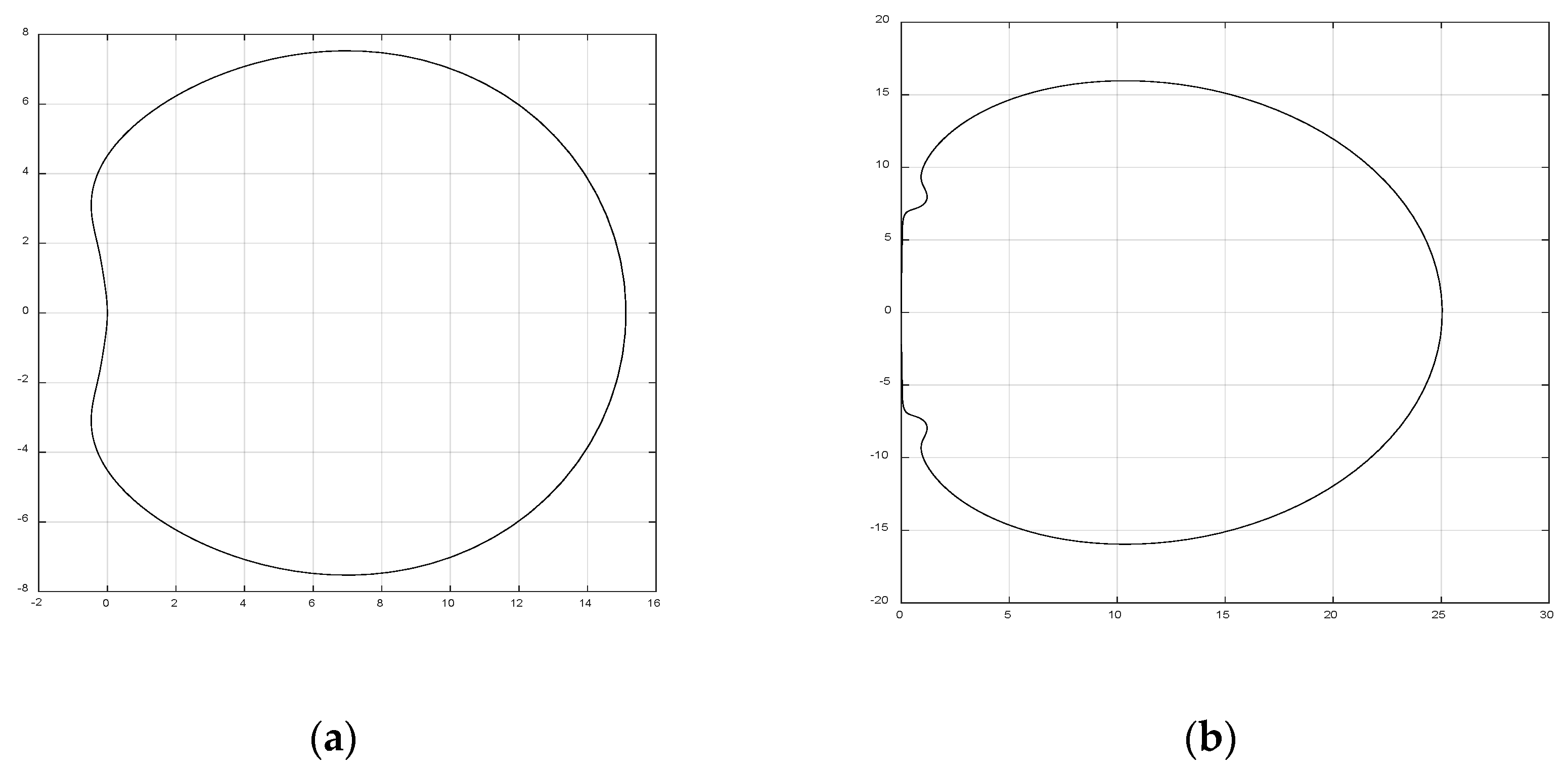
4. Regions of Absolute Stability (RAS) of the Block Hybrid Methods

Generally, in designing a new numerical method, it is very important to consider the stability properties of the method. Therefore, in this paper, we reformulate the block hybrid methods, as in [31,32], by the partitioning $(s+r)\times (s+r)$ of the form

$$\left[\begin{array}{l}{Y}^{\left[n\right]}\\ y^{\left[n-1\right]}\end{array}\right]=\left[\frac{A|\hspace{0.17em}U}{B\hspace{0.17em}|\hspace{0.17em}V}\right]\left[\begin{array}{l}hf\left(Y^{\left[n\right]}\right)\\ y^{\left[n\right]}\end{array}\right], n=1, 2, \dots , \mathrm{N},$$

(22a)

where

$$Y^{\left[n\right]}=\left[\begin{array}{c}{Y}_1^{\left[n\right]}\\ Y_2^{\left[n\right]}\\ ⋮\\ Y_s^{\left[n\right]}\end{array}\right], y^{\left[n-1\right]}=\left[\begin{array}{c}{y}_1^{\left[n-1\right]}\\ y_2^{\left[n-1\right]}\\ ⋮\\ y_r^{\left[n-1\right]}\end{array}\right], f\left(Y^{\left[n\right]}\right)=\left[\begin{array}{c}f(Y_1^{\left[n\right]})\\ f(Y_2^{\left[n\right]})\\ ⋮\\ f(Y_s^{\left[n\right]})\end{array}\right], y^{\left[n\right]}=\left[\begin{array}{c}{y}_1^{\left[n\right]}\\ y_2^{\left[n\right]}\\ ⋮\\ y_r^{\left[n\right]}\end{array}\right],$$

$$A=\left[\begin{array}{c}0\hspace{0.17em}\hspace{0.17em}\hspace{0.17em}\hspace{0.17em}\hspace{0.17em}\hspace{0.17em}\hspace{0.17em}0\\ A\hspace{0.17em}\hspace{0.17em}\hspace{0.17em}\hspace{0.17em}\hspace{0.17em}\hspace{0.17em}\hspace{0.17em}B\end{array}\right], U=\left[\begin{array}{c}I\hspace{0.17em}\hspace{0.17em}\hspace{0.17em}\hspace{0.17em}\hspace{0.17em}\hspace{0.17em}\hspace{0.17em}0\hspace{0.17em}\hspace{0.17em}\hspace{0.17em}\hspace{0.17em}\hspace{0.17em}\hspace{0.17em}\hspace{0.17em}0\\ 0\hspace{0.17em}\hspace{0.17em}\hspace{0.17em}\hspace{0.17em}\hspace{0.17em}\hspace{0.17em}\hspace{0.17em}\mu \hspace{0.17em}\hspace{0.17em}\hspace{0.17em}\hspace{0.17em}\hspace{0.17em}\hspace{0.17em}\hspace{0.17em}e-\mu \end{array}\right], B=\left[\begin{array}{c}A\hspace{0.17em}\hspace{0.17em}\hspace{0.17em}\hspace{0.17em}\hspace{0.17em}\hspace{0.17em}\hspace{0.17em}B\\ 0\hspace{0.17em}\hspace{0.17em}\hspace{0.17em}\hspace{0.17em}\hspace{0.17em}\hspace{0.17em}\hspace{0.17em}0\\ {\nu }^T\hspace{0.17em}\hspace{0.17em}\hspace{0.17em}\hspace{0.17em}\hspace{0.17em}\hspace{0.17em}\hspace{0.17em}{\omega }^T\end{array}\right], V=\left[\begin{array}{c}I\hspace{0.17em}\hspace{0.17em}\hspace{0.17em}\hspace{0.17em}\hspace{0.17em}\hspace{0.17em}\hspace{0.17em}\mu \hspace{0.17em}\hspace{0.17em}\hspace{0.17em}\hspace{0.17em}\hspace{0.17em}\hspace{0.17em}\hspace{0.17em}e-\mu \\ 0\hspace{0.17em}\hspace{0.17em}\hspace{0.17em}\hspace{0.17em}\hspace{0.17em}\hspace{0.17em}\hspace{0.17em}0\hspace{0.17em}\hspace{0.17em}\hspace{0.17em}\hspace{0.17em}\hspace{0.17em}\hspace{0.17em}\hspace{0.17em}I\\ 0\hspace{0.17em}\hspace{0.17em}\hspace{0.17em}\hspace{0.17em}\hspace{0.17em}\hspace{0.17em}\hspace{0.17em}0\hspace{0.17em}\hspace{0.17em}\hspace{0.17em}\hspace{0.17em}\hspace{0.17em}\hspace{0.17em}\hspace{0.17em}I-\theta \end{array}\right],$$

and $e={[1,\cdots ,1]}^T\in R^m$.

Thus, Equation (22a) is

$$\left[\begin{array}{c}{Y}_1^{\left[n\right]}\\ Y_2^{\left[n\right]}\\ ⋮\\ Y_s^{\left[n\right]}\\ -\\ y_1^{[n]}\\ ⋮\\ y_r^{[n]}\end{array}\right]=\left[\frac{A\hspace{0.17em}\hspace{0.17em}|\hspace{0.17em}\hspace{0.17em}U}{B\hspace{0.17em}\hspace{0.17em}|\hspace{0.17em}\hspace{0.17em}V}\right]\hspace{0.17em}\hspace{0.17em}\left[\begin{array}{c}hf(Y_1^{\left[n\right]})\\ hf(Y_2^{\left[n\right]})\\ ⋮\\ hf(Y_s^{\left[n\right]})\\ -\\ y_1^{[n-1]}\\ ⋮\\ y_r^{[n-1]}\end{array}\right].$$

(22b)

The values r and s denote output and stage values, respectively. Applying Equation (22) to the linear test equation $y^{\prime }=\lambda y,$$x\ge 0$ and $\lambda \in C$, we have $M(z)$ as

$$M(z)=V+zB{(1-zA)}^{-1}U$$

(23)

and the stability polynomial $\rho \left(\eta ,z\right)$ of the method can easily be obtained as

$$\rho \left(\eta ,z\right)=det\left(\eta I-M\left(z\right)\right).$$

(24)

The region of absolute stability $\Re$ of the method is defined as

$$\Re =x\in C:\rho (\eta ,z)=1\Rightarrow \left|\eta \right|\le 1.$$

Computing the stability function gives the stability polynomial of the method, which is plotted to produce the required graph of the region of absolute stability of the method, as shown in Figure 2.

Remark 1.

In the stable block hybrid second-derivative implicit method, we added the matrix D1 obtained from the coefficients of$h^2$to the matrices A, C, B, and D, which enabled us to plot the region of absolute stability of the new method. The region of absolute stability of method (18) is A($\alpha$)-stable while the region of absolute stability of the second-derivative implicit method (21) is A-stable since the region contains the complex plane outside the enclosed figure.

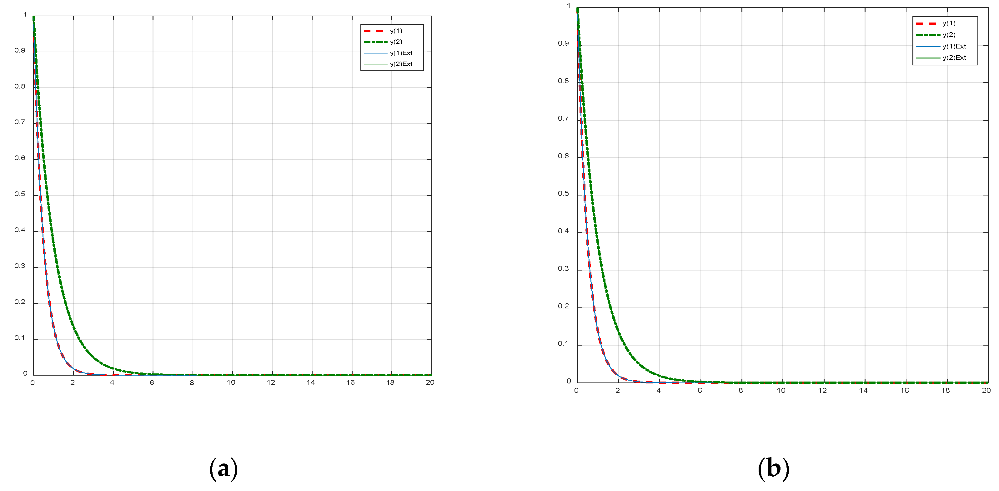
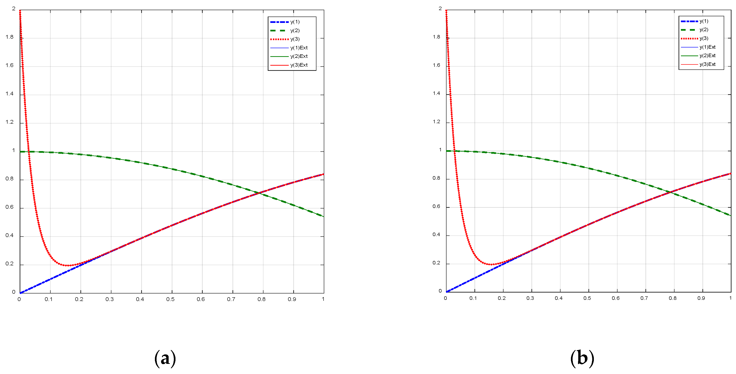
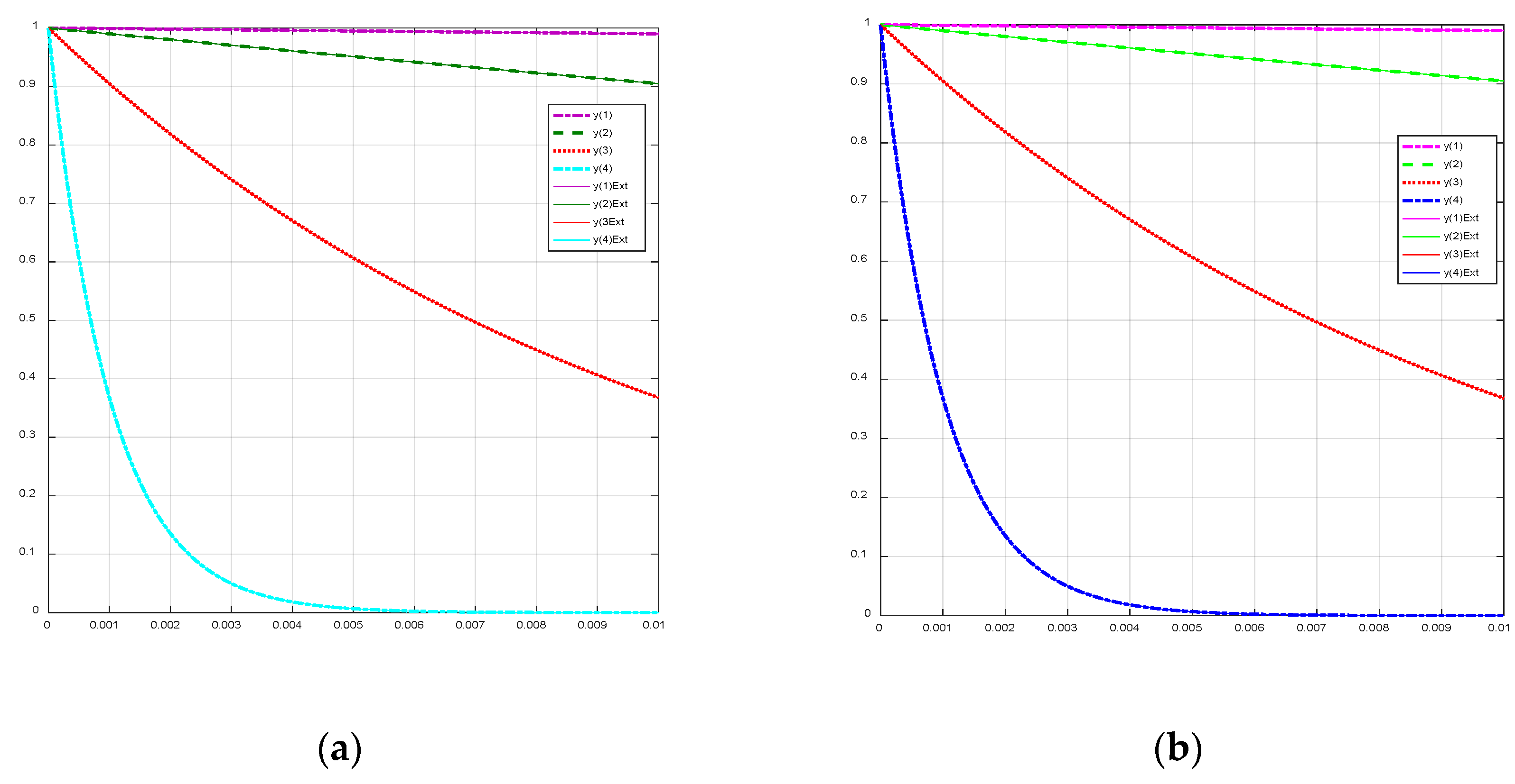
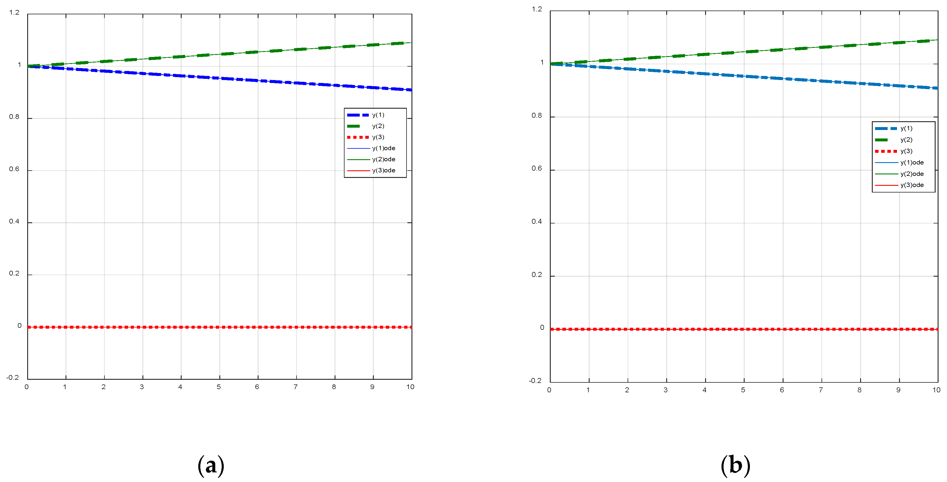
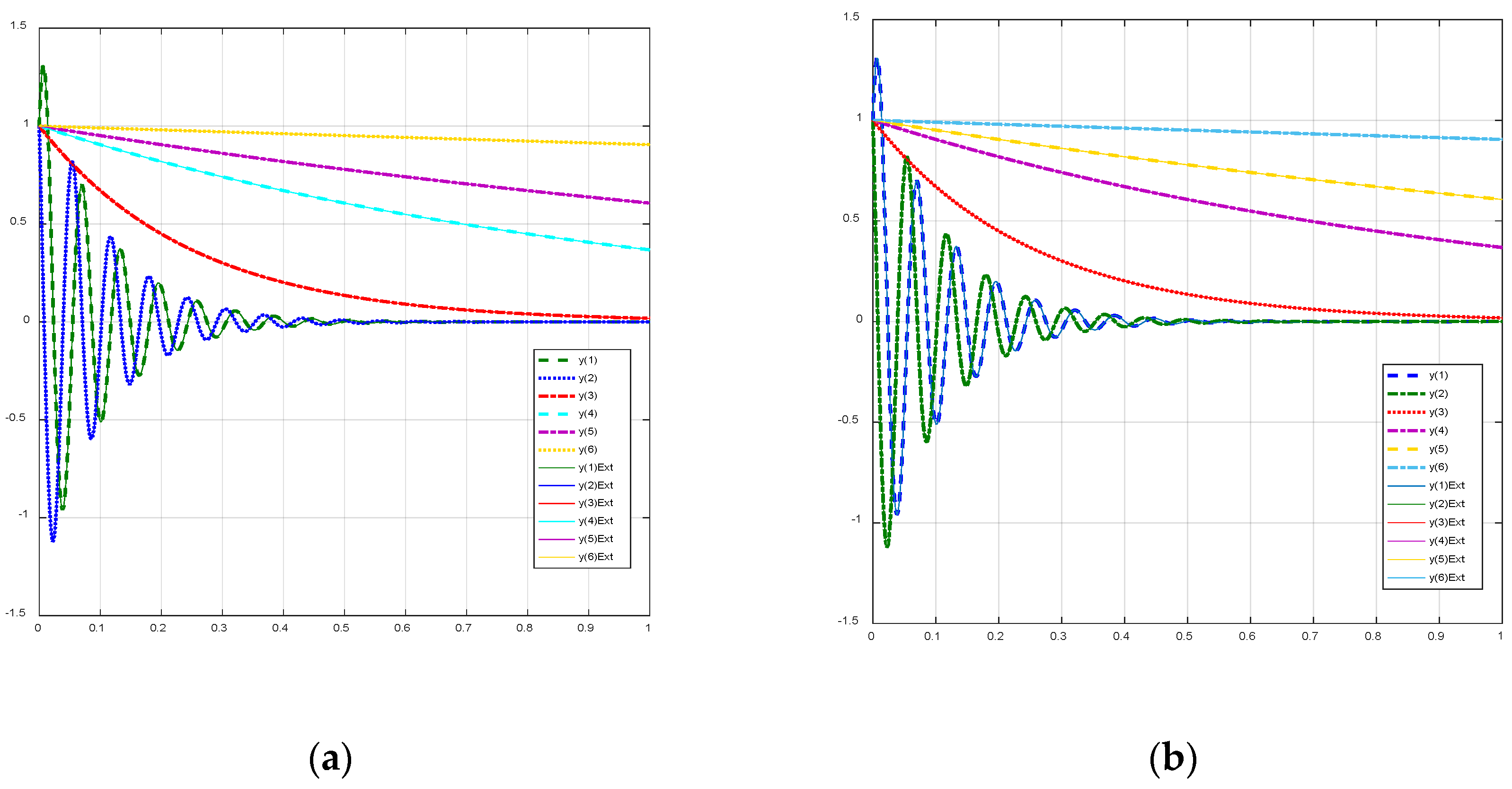
5. Numerical Illustrations

For the illustration of the performance of the derived methods, we consider both linear and nonlinear challenging systems. To provide a direct comparison, Matlab software codes were written for the preliminary test experiments using a fixed step length. We present the calculated results in tables and depict the curves in figures. Here, nfe and Ext are the function evaluations and exact values, respectively.

Example 1.

The Kaps problem [30].

We consider the nonlinear Kaps stiff system,

$$\left[\begin{array}{l}{y^{\prime }}_1(x)\\ {y^{\prime }}_2(x)\end{array}\right]=\left[\begin{array}{l}-1002 y_1(x)+1000 y_2^2(x)\\ y_1(x)-y_2(x)(1+y_2(x))\end{array}\right],\hspace{1em}\hspace{1em}\left[\begin{array}{l}{y}_1(0)\\ y_2(0)\end{array}\right]=\left[\begin{array}{l}1\\ 1\end{array}\right].$$

The exact value of the system is

$$\left[\begin{array}{l}{y}_1(x)\\ y_2(x)\end{array}\right]=\left[\begin{array}{l}\exp (-2x)\\ \exp (-x)\end{array}\right].$$

The solutions of this example are shown in

Table 2. Absolute errors in the numerical integration of example 1.

x	${\mathit{y}}_{\mathit{i}}$	Method (18)	Method (21)
	$y_1$	1.223052805026881 × 10−3	1.228938367083599 × 10−3
5	$y_2$	1.290570363021715 × 10−6	1.800318343625484 × 10−6
	$y_1$	3.320709446422848 × 10−5	3.325679258575631 × 10−5
50	$y_2$	9.887815172193726 × 10−8	5.804723043345561 × 10−7
	$y_1$	3.619658989642897 × 10−12	3.622719245691676 × 10−12
250	$y_2$	2.523305960607913 × 10−11	2.101212666995355 × 10−10
	$y_1$	7.167561881971770 × 10−21	7.173620185942641 × 10−21
500	$y_2$	1.122741130992365 × 10−15	9.350493168888896 × 10−15

and the solution curves are depicted in Figure 3.

Example 2.

Consider the linear stiff system.

$$\left[\begin{array}{l}{y^{\prime }}_1(x)\\ {y^{\prime }}_2(x)\\ {y^{\prime }}_3(x)\end{array}\right]=\left[\begin{array}{lll}0& \hspace{0.17em}1& \hspace{0.17em}0\\ -1& \hspace{0.17em}0& \hspace{0.17em}0\\ 25& \hspace{0.17em}1& \hspace{0.17em}-25\end{array}\right]\left[\begin{array}{l}{y}_1(x)\\ y_2(x)\\ y_3(x)\end{array}\right],\left[\begin{array}{l}{y}_1(0)\\ y_2(0)\\ y_3(0)\end{array}\right]=\left[\begin{array}{l}0\\ 1\\ 2\end{array}\right].$$

The exact value is

$$\left[\begin{array}{c}{y}_1\left(x\right)\\ y_2\left(x\right)\\ y_3\left(x\right)\end{array}\right]=\left[\begin{array}{l}sin(x)\\ cos(x)\\ sin(x)+2 exp(Lx)\end{array}\right].$$

The results of using the newly constructed methods are shown in

Table 3. Absolute errors in the numerical integration of example 2.

x	${\mathit{y}}_{\mathit{i}}$	Method (18)	Method (21)
	$y_1$	0	0
5	$y_2$	1.110223024625157 × 10−16	1.110223024625157 × 10−16
	$y_3$	7.993605777301127 × 10−15	0
	$y_1$	5.551115123125783 × 10−17	4.163336342344337 × 10−17
50	$y_2$	3.330669073875470 × 10−16	3.330669073875470 × 10−16
	$y_3$	1.038058528024521 × 10−14	0
	$y_1$	2.220446049250313 × 10−16	1.110223024625157 × 10−16
250	$y_2$	1.110223024625157 × 10−16	1.110223024625157 × 10−16
	$y_3$	3.330669073875470 × 10−16	1.665334536937735 × 10−16
	$y_1$	4.440892098500626 × 10−16	3.330669073875470 × 10−16
500	$y_2$	2.220446049250313 × 10−16	1.110223024625157 × 10−16
	$y_3$	3.330669073875470 × 10−16	2.220446049250313 × 10−16

and the solution curves are in Figure 4.

Example 3.

The linear problem by Enright [33] is given by:

$$\left[\begin{array}{l}{y^{\prime }}_1(x)\\ {y^{\prime }}_2(x)\\ {y^{\prime }}_3(x)\\ {y^{\prime }}_4(x)\end{array}\right]=\left[\begin{array}{llll}-1& \hspace{1em}0& \hspace{1em}0& \hspace{1em}0\\ 0& \hspace{1em}-10& \hspace{1em}0& \hspace{1em}0\\ 0& \hspace{1em}0& \hspace{1em}-100& \hspace{1em}0\\ 0& \hspace{1em}0& \hspace{1em}0& \hspace{1em}-1000\end{array}\right]\left[\begin{array}{l}{y}_1(x)\\ y_2(x)\\ y_3(x)\\ y_4(x)\end{array}\right],\hspace{0.17em}\hspace{0.17em}\hspace{0.17em}\hspace{0.17em}\left[\begin{array}{l}{y}_1(0)\\ y_2(0)\\ y_3(0)\\ y_4(0)\end{array}\right]=\left[\begin{array}{l}1\\ 1\\ 1\\ 1\end{array}\right].$$

The results of the integration are largely self-explanatory. If we examine the accuracy obtained, however, we see that the newly constructed methods are considerably accurate (see

Table 4. Absolute errors in the numerical integration of example 3.

x	${\mathit{y}}_{\mathit{i}}$	Method (18)	Method (21)
	$y_1$	0	0
5	$y_2$	0	0
	$y_3$	0	0
	$y_4$	1.110223024625157 × 10−16	1.110223024625157 × 10−16
	$y_1$	2.220446049250313 × 10−16	2.220446049250313 × 10−16
50	$y_2$	4.440892098500626 × 10−16	4.440892098500626 × 10−16
	$y_3$	1.110223024625157 × 10−16	1.110223024625157 × 10−16
	$y_4$	2.220446049250313 × 10−16	1.110223024625157 × 10−16
	$y_1$	5.551115123125783 × 10−16	5.551115123125783 × 10−16
250	$y_2$	7.771561172376096 × 10−16	7.771561172376096 × 10−16
	$y_3$	7.771561172376096 × 10−16	1.110223024625157 × 10−16
	$y_4$	5.204170427930421 × 10−18	5.204170427930421 × 10−18
	$y_1$	2.220446049250313 × 10−16	2.220446049250313 × 10−16
500	$y_2$	5.551115123125783 × 10−16	5.551115123125783 × 10−16
	$y_3$	3.885780586188048 × 10−16	2.775557561562891 × 10−16
	$y_4$	1.626303258728257 × 10−19	3.388131789017201 × 10−20

). The plotted curves are displayed in Figure 5.

Example 4.

This is given by Gear [34]:

$$\begin{array}{l}{y^{\prime }}_1==-0.013 y_1-1000 y_1{y}_3,\hspace{1em}\hspace{1em}\hspace{1em}\hspace{1em}\hspace{1em}\hspace{1em}{y}_1(0)=1,\\ {y^{\prime }}_2=-2500 y_2{y}_3,\hspace{1em}\hspace{1em}\hspace{1em}\hspace{1em}\hspace{1em}\hspace{1em}\hspace{1em}\hspace{1em}\hspace{1em}\hspace{1em} y_2(0)=1,\\ {y^{\prime }}_3=-0.013 y_1-1000 y_1{y}_3-2500 y_2{y}_3,\hspace{1em}\hspace{1em} y_3(0)=0\hspace{0.17em}.\end{array}$$

We solve this problem, and the solution curves are presented in Figure 6.

Example 5.

Here, the present problem was solved by [35]. Therefore, for comparison, we present the graphical plots of this example in Figure 7, comparing with the exact solution curves. The application of the newly derived methods to this problem is to demonstrate their performance. However, we considered only the first four components$\left\{y_1,y_2,y_3,y_4\right\}$, as shown in

Table 5. Absolute errors of numerical integration of example 5.

x	yi	Method (18)	Method (21)
	$y_1$	2.024105327791403 × 10−10	2.220446049250313 × 10−16
	$y_2$	4.056337835067758 × 10−10	1.318389841742373 × 10−16
5	$y_3$	0	0
	$y_4$	0	0
	$y_1$	1.721994824510631 × 10−9	3.330669073875470 × 10−16
	$y_2$	1.453979242560521 × 10−9	7.771561172376096 × 10−16
50	$y_3$	4.440892098500626 × 10−16	4.440892098500626 × 10−16
	$y_4$	0	1.110223024625157 × 10−16
	$y_1$	2.077217382476237 × 10−10	6.591949208711867 × 10−17
	$y_2$	1.233960850166582 × 10−11	1.734723475976807 × 10−18
250	$y_3$	2.775557561562891 × 10−17	8.326672684688674 × 10−17
	$y_4$	6.661338147750939 × 10−16	6.661338147750939 × 10−16
	$y_1$	2.711908290569135 × 10−12	6.810144895924575 × 10−19
	$y_2$	6.195955749334348 × 10−13	2.710505431213761 × 10−20
500	$y_3$	6.938893903907228 × 10−18	4.857225732735060 × 10−17
	$y_4$	3.885780586188048 × 10−16	3.330669073875470 × 10−16

.

$$\left[\begin{array}{l}{y^{\prime }}_1(x)\\ {y^{\prime }}_2(x)\\ {y^{\prime }}_3(x)\\ {y^{\prime }}_4(x)\\ {y^{\prime }}_5(x)\\ {y^{\prime }}_6(x)\end{array}\right]=\left[\begin{array}{llllll}-10& \hspace{1em}100& \hspace{1em}0& \hspace{1em}0& \hspace{1em}0& \hspace{1em}0\\ -100& \hspace{1em}-10& \hspace{1em}0& \hspace{1em}0& \hspace{1em}0& \hspace{1em}0\\ 0& \hspace{1em}0& \hspace{1em}-4& \hspace{1em}0& \hspace{1em}0& \hspace{1em}0\\ 0& \hspace{1em}0& \hspace{1em}0& \hspace{1em}-1& \hspace{1em}0& \hspace{1em}0\\ 0& \hspace{1em}0& \hspace{1em}0& \hspace{1em}0& \hspace{1em}-0.5& \hspace{1em}0\\ 0& \hspace{1em}0& \hspace{1em}0& \hspace{1em}0& \hspace{1em}0& \hspace{1em}-0.1\end{array}\right]\left[\begin{array}{l}{y}_1(x)\\ y_2(x)\\ y_3(x)\\ y_4(x)\\ y_5(x)\\ y_6(x)\end{array}\right],\hspace{0.17em}\hspace{0.17em}\left[\begin{array}{l}{y}_1(0)\\ y_2(0)\\ y_3(0)\\ y_4(0)\\ y_5(0)\\ y_6(0)\end{array}\right]=\hspace{0.17em}\hspace{0.17em}\hspace{0.17em}\hspace{0.17em}\left[\begin{array}{l}1\\ 1\\ 1\\ 1\\ 1\\ 1\end{array}\right]\hspace{0.17em}$$

6. Concluding Remarks

The presented second-derivative block hybrid method for a stiff system of ordinary differential equations is suitable for large systems. The second-derivative block hybrid time integrator provides good performance. Numerical results for the new second-derivative block hybrid method are promising and are demonstrably comparable to those obtained from popular high-order stiff time integrators found in the literature. Their stability properties, based on Remark 1, indicate that they are good candidates for large stiff systems. The next step of our research is to further apply some new methods to modeled differential equations that arise in other areas of scientific fields, such as chemical reaction, enzyme kinetics, cardiac electrophysiology, models of drug magnetic nanoparticle transport, and a model of tumor immune interaction, to mention just a few.

References

1. Onumanyi, P.; Awoyemi, D.O.; Jator, S.N.; Sirisena, U.W. New linear multi-step methods with continuous coefficients for first order initial value problems. J. Nig. Math. Soc. 1994, 13, 37–51. [Google Scholar]
2. Chollom, J.P.; Jackiewicz, Z. Construction of two step Runge-Kutta (TSRK) methods with large regions of absolute stability. J. Compt. Appl. Math. 2003, 157, 125–137. [Google Scholar] [CrossRef] [Green Version]
3. Chollom, J.P.; Onumanyi, P. Variable order A-stable Adams Moulton type block hybrid methods for solution of stiff first order ODEs. J. Math. Assoc. Niger. Abacus (31) B 2004, 2, 177–192. [Google Scholar]
4. Jator, S.N. Leaping type of algorithm for parabolic partial differential equations. JMS Natl. Math. Cent. Abuja Niger. 2013, 2, 149–172. [Google Scholar]
5. Gragg, W.B.; Stetter, H.J. Generalized multistep predictor-corrector methods. J. Assoc. Comput. Mach. 1964, 11, 188–209. [Google Scholar] [CrossRef]
6. Butcher, J.C. Modified multistep method for the numerical integration of ordinary differential equations. J. Assoc. Comput. Mach. 1965, 12, 124–135. [Google Scholar] [CrossRef]
7. Butcher, J.C. A multistep generalization of Runge-Kutta method with four or five stages. J. Ass. Comput. Mach. 1967, 14, 84–99. [Google Scholar] [CrossRef]
8. Gear, W.C. Hybrid multistep method for initial value in ordinary differential equations. J. SIAM Numer. Anal. 1965, 2, 69–86. [Google Scholar]
9. Urabe, M. An implicit one-step method of high-order accuracy for the numerical integration of ordinary differential equations. J. Numer. Math. 1970, 15, 151–164. [Google Scholar] [CrossRef]
10. Mitsui, T. A modified version of Urabe’s implicit single-step method. J. Comp. Appl. Math. 1987, 20, 325–332. [Google Scholar] [CrossRef] [Green Version]
11. Cash, J.R. High order methods for the numerical integration of ordinary differential equations. Numer. Math. 1978, 30, 385–409. [Google Scholar] [CrossRef]
12. Gupta, G.K. Implementing second-derivative multistep methods using the Nordsieck polynomial representation. J. Math. Comput. 1978, 32, 13–18. [Google Scholar] [CrossRef]
13. Shintani, H. On one-step methods utilizing the second derivative. Hiroshima Math. J. 1971, 1, 349–372. [Google Scholar] [CrossRef]
14. Shintani, H. On explicit one-step methods utilizing the second derivative. Hiroshima Math. J. 1972, 2, 353–368. [Google Scholar] [CrossRef]
15. Mitsui, T. Runge-Kutta type integration formulas including the evaluation of the second-derivative, Part I. Publ. Res. Inst. Math. Sci. 1982, 18, 325–364. [Google Scholar] [CrossRef] [Green Version]
16. Chan, R.P.K.; Tsai, A.Y.J. On explicit two-derivative Runge-Kutta methods. Numer. Algorithm 2010, 53, 171–194. [Google Scholar] [CrossRef]
17. Marian, D.; Ciplea, S.A.; Lungu, N. On the Ulam-Hyers Stability of Biharmonic Equation. Univ. Politeh. Buchar. Sci. Bull.-Ser. A-Appl. Math. Phys. 2020, 8, 141–148. [Google Scholar]
18. Shokri, A. The Symmetric P-Stable Hybrid Obrenchkoff Methods for the numerical solution of second Order IVPS. TWMS J. Pure Appl. Math. 2012, 5, 28–35. [Google Scholar]
19. Shokri, A. An explicit trigonometrically fitted ten-step method with phase-lag of order infinity for the numerical solution of the radial Schrödinger equation. J. Appl. Comput. Math. 2015, 14, 63–74. [Google Scholar]
20. Shokri, A.; Saadat, H. P-stability, TF and VSDPL technique in Obrechkoff methods for the numerical solution of the Schrödinger equation. Bull. Iran. Math. Soc. 2016, 42, 687–706. [Google Scholar]
21. Marian, D.; Ciplea, S.A.; Lungu, N. Ulam-Hyers stability of Darboux-Ionescu problem. Carpathian J. Math. 2021, 37, 211–216. [Google Scholar] [CrossRef]
22. Sunday, J.; Shokri, A.; Marian, D. Variable step hybrid block method for the approximation of Kepler problem. Fractal Fract. 2022, 6, 343. [Google Scholar] [CrossRef]
23. Kwami, A.M.; Kumleng, G.M.; Kolo, A.M.; Yakubu, D.G. Block hybrid multistep methods for the numerical integration of stiff systems of ordinary differential equations arising from chemical reactions. Abacus J. Math. Assoc. Nig. 2015, 42, 134–164. [Google Scholar]
24. Singh, G.; Garg, A.; Kanwar, V.; Ramos, H. An efficient optimized adaptive step-size hybrid block method for integrating differential systems. Appl. Math. Comp. 2019, 362, 124567. [Google Scholar] [CrossRef]
25. Yakubu, D.G.; Aminu, M.; Tumba, P.; Abdulhameed, M. An efficient family of second-derivative Runge-Kutta collocation methods for oscillatory systems. J. Nig. Math. Soc. 2018, 37, 111–138. [Google Scholar]
26. Chu, M.T.; Hamilton, H. Parallel solution of ordinary differential equations by multi-block methods. SIAM J. Sci. Stat. Comp. 1987, 8, 342–353. [Google Scholar] [CrossRef]
27. Yakubu, D.G.; Aminu, M.; Aminu, A. The numerical integration of stiff systems using stable multistep multi-derivative methods. Mod. Meth. Numer. Math. 2017, 8, 99–117. [Google Scholar] [CrossRef] [Green Version]
28. Fatunla, S.O. Block methods for second order ODEs. Intern. J.Comput. Math. 1991, 41, 55–63. [Google Scholar] [CrossRef]
29. Lambert, J.D. Computational Methods in Ordinary Differential Equations; John Willey and Sons: New York, NY, USA, 1973. [Google Scholar]
30. Lambert, J.D. Numerical Methods for Ordinary Differential Systems; John Wiley: New York, NY, USA, 1991. [Google Scholar]
31. Burrage, K.; Butcher, J.C. Non-linear stability for a general class of differential equation method. BIT Numer. Math. 1980, 20, 185–203. [Google Scholar] [CrossRef]
32. Butcher, J.C. Numerical Methods for Ordinary Differential Equations, 2nd ed.; John Wiley & Sons, Ltd.: New York, NY, USA, 2008. [Google Scholar]
33. Enright, W.H. Second derivative multistep methods for stiff ordinary differential equations. SIAM J. Numer. Anal. 1974, 11, 321–341. [Google Scholar] [CrossRef]
34. Gear, W.C. DIFSUB for Solution of ordinary differential equations. Comm. ACM 1971, 14, 185–190. [Google Scholar] [CrossRef]
35. Fatunla, S.O. Numerical integrators for stiff and highly oscillatory differential equations. J. Math. Comput. 1980, 34, 373–390. [Google Scholar] [CrossRef]
Figure 1. Schematic representation of the block hybrid methods for stiff system of initial value problems.
Fractalfract 06 00386 g001
Figure 2. Regions of absolute stability of the block hybrid methods. (a) Method (18) is A( α )-stable. (b) Method (21) is A-stable.
Fractalfract 06 00386 g002
Figure 3. Graphical plots of Example 1 using block hybrid methods with nfe = 500. (a) Solution curve of Example 1 using (18); (b) solution curve of Example 1 using (21).
Fractalfract 06 00386 g003
Figure 4. Graphical plots of Example 2 using block hybrid methods with nfe = 500. (a) Solution curve of Example 2 using (18); (b) solution curve of Example 2 using (21).
Fractalfract 06 00386 g004
Figure 5. Graphical plots of Example 3 using block hybrid methods with nfe = 500. (a) Solution curve of Example 3 using (18); (b) solution curve of Example 3 using (21).
Fractalfract 06 00386 g005
Figure 6. Graphical plots of Example 4 using the block hybrid methods with nfe = 500. (a) Solution curve of Example 4 using (18); (b) solution curve of Example 4 using (21).
Fractalfract 06 00386 g006
Figure 7. Graphical plots of Example 5 using block hybrid methods with nfe = 500. (a) Solution curve of Example 5 using method (18); (b) solution curve of Example 5 using method (21).
Fractalfract 06 00386 g007