Deflection of Beams Modeled by Fractional Differential Equations

Abstract

Using the concept of a fractional derivative, in Caputo’s sense, we derive and solve a fractional differential equation that models the deflection of beams. The scheme to introduce the fractional concept can be used for different situations; in the article, we only consider four cases as an example of its usefulness. In addition, we establish a relationship between the fractional index and the level of stiffness (or flexibility) of the material with which the beam is made.

1. Introduction

In applied mathematics, the study of beam deflection is one of the main issues due to the implications regarding the safety of structures, see for example [1,2]. Because this is important, without a doubt, we must consider more general models that consequently involve more factors in the model. In this way, models closer to reality are obtained. In order to increase the “toolbox”, that is, models, in the present work fractional differential equations are deduced, in the sense of Caputo, to model the deflection of beams.

It is known in the literature [3] that the fractional calculation is an effective mathematical entity to model phenomena where the viscoelasticity of certain materials intervenes, even more so the fractional index of the equation in this case is related to the memory of the material. Therefore, it is natural to consider fractional calculus to model the beam deflection phenomena. Indeed, as we will see, in our case, the index of the differential equation is related to the stiffness (or respectively elasticity) of the material with which the beam in question is made. In fact, certain materials, such as wood or PVC plastics, become more rigid with climate changes, such as solar radiation or acid rain. Or, they become more flexible, for example with heat, see [4]. In this way, we see that the fractional calculation is a useful means of modeling real phenomena, see [5,6], that could be very important for some sciences as civil engineering, for example.

At present, there is a great diversity of fractional derivatives, and among the classical derivatives are the Riemann–Liouville derivatives, which are frequently used in real analysis or calculus, the derivatives in the sense of Caputo, which are used, for example, in numerical analysis and in physics, and there are also derivatives in the Grunwald–Letnikov sense that are used in signal processing and control theory, among many others. In our case, we have chosen the derivative in the sense of Caputo because the derivative of constant functions is zero and because the order of the derivative, in the differential equations that we are going to consider, is an integer in the initial conditions. As we have commented, the use of the derivative in the sense of Caputo is frequently used because, for example, there is no ambiguity in the interpretation of the concept of fractional derivatives in the initial conditions, since they coincide with the classic case, that is, they are integers. This fact does not occur with all fractional derivatives; however, in some cases, attempts have been made to give it a physical meaning. In our opinion, we believe that there is nothing definitive (see for example [7,8,9]) and all fractional calculation is a current area of applied and pure mathematics, [10,11,12,13].

It is common, in the classical case, to use differentials in modeling real phenomenon, that is, small increases $\mathsf{\Delta }x$ in the independent variable are considered to produce an increase $\mathsf{\Delta }y=f(x+\mathsf{\Delta }x)-f\left(x\right)$ in the dependent variable, for some given function f. If the function f is differentiable, then $\mathsf{\Delta }y$ is approximately $f^{\prime }\left(x\right)\mathsf{\Delta }x$. It should be noted that this property ceases to hold in the fractional sense. That is, the increment $\mathsf{\Delta }y$ is no longer proportional to $f^{\left(\alpha \right)}\left(x\right)\mathsf{\Delta }x$, where $f^{\left(\alpha \right)}\left(x\right)$ is the $\alpha$-order fractional derivative of f, in one of the three senses mentioned before. As is known, this is a major obstacle in the derivation of fractional models and there is a great variety of methods to solve this problem, see for example [14,15,16]. In our case, to derive the fractional differential equation we proceed, broadly speaking, from the following way. We fix an arbitrary point x and, to derive the fractional differential equation, we consider a local approximation of the solution in x and we derive it in the sense of Caputo (here it comes into play that the derivative of constant functions is zero), and then we evaluate it in x. For more details, see for example the derivation of Equation (11).

On the other hand, it should be noted that in the classical derivation of the beam equation, as in the fractional calculus, the use of the chain rule is required. While it is true that the chain rule exists for some fractional derivatives, it is also true that such chain rules are of little or no use, since the derivative of a composition of functions implies the classical derivative of the functions of all orders, plus there is the fact that the resulting expression is not easy to apply, see for example [8,9].

In addition, in the literature, there are many derivatives that are said to be fractional but are not, since they retain the local character of the classical derivative, see for example [17]. For these pseudo-fractional derivatives, a certain complicated type of the chain rule is known, see for example [18,19]. However, our interest is that the non-local character of the beam deflection phenomenon enters, in some sense, into the model that we are going to consider. For example, if some force is applied to the beam at a certain point, then the beam has in some sense memory of that force. Conversely, we want the environment surrounding the beam to exert some change in its stiffness or flexibility. The problem here is that there is no fractional derivative (that is, a non-local derivative) that is zero for constant functions and that also satisfies the chain rule, see [20,21]. This difficulty is overcome by approximations of the solution, see for example the approximation (10).

In this way, in this paper we use the fractional derivative in the sense of Caputo to model different schemes of hanging beams (there is a great variety of schemes, see [22]). In the model, we note that the index of the fractional equation is a measure of the stiffness-deflection of the beam that can be acquired over time due to climatic factors (see Examples 1 and 3 below). Or, if some force is applied to it, then the fractional index in the equation can be a memory indicator of the force applied to the beam (see Examples 2 and 4 below).

The article is organized in the following manner. In Section 2, we briefly recall the derivation of the classical beam equation, this will help us to introduce some notations used in the fractional model. Next, in Section 3 and Section 4 we present some auxiliary results of the fractional calculus in the sense of Caputo and we deduce the fractional equation of the beam, respectively. As an application example, in Section 5 we present the deduction of four fractional equations with their corresponding analytical solutions. Later, in Section 6 we give numerical examples of the respective four analytical examples that illustrate the application of the fractional model. Finally, in Section 7 we conclude, giving some final comments and possible applications of the methodology developed here.

2. Classical Equation for the Deflection of a Beam

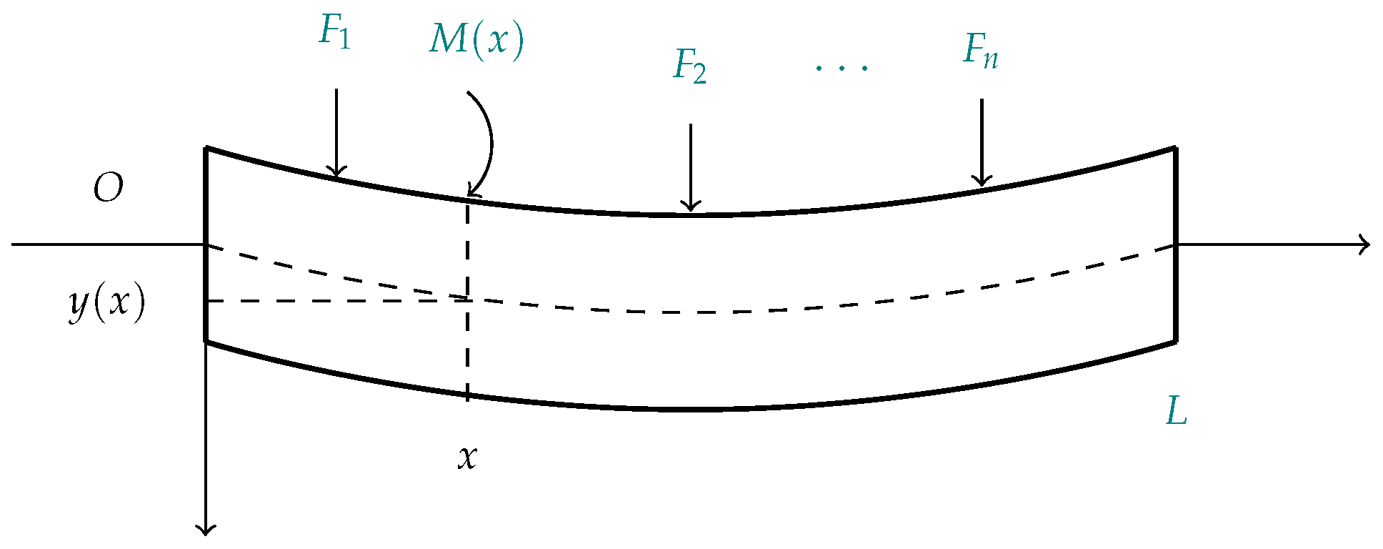
Due to the fact that it is convenient to introduce some concepts that will help us to understand the fractional model, next we briefly recall the classical deduction of the equation of a beam. For a detailed deduction, you can consult [23], for example. Suppose that an elastic beam is subjected to different forces, $F_1,...,F_n$, and due to them it deforms, see Figure 1. The curve resulting in the center of the beam is called elastic curve $y\left(x\right)$, and its determination is important to several areas of applied science. In what follows, we introduce some concepts to derive the elastic curve. Without loss of generality, we consider an elastic beam placed in the segment $OL$, O is the origin of coordinates and L its longitude. We will take as positive to the right of the origin O and as negative down from the origin. In this way, the forces applied to the beam, and its downward displacement, are considered positive. Let $M\left(x\right)$ be the bending moment in a vertical cross section of the beam at point x, that is, $M\left(x\right)$ is a measure of the tendency of forces to bend or twist the beam at point x. The displacement of the axis of symmetry $OL$, at point x, is called deflection of the beam and is denoted by $y\left(x\right)$, this is what determines the elastic curve of the beam, see Figure 1.

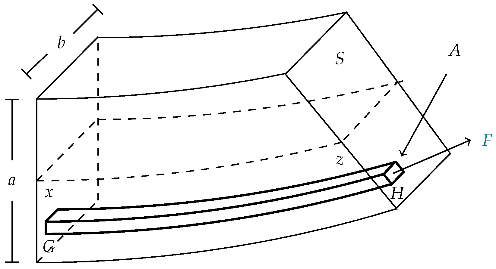
Suppose further that the beam is a units high and b units wide. That is, it has a cross-sectional area S of $ab$ square units. Let us consider an element of the beam between the points x and z, with z greater than x, but very close to x (notice that we avoid the use of differentials). Moreover, let $GH$ be a small rectangular fiber with a cross-sectional of area A that is below the elastic curve, see Figure 2.

Suppose the beam element at its midsection has length l, and let $\tilde{l}-l$ be the part of the beam that was elongated due to a perpendicular force F acting on area A. The moment of this force about the section mean is

$$M=uF,$$

(1)

where u is the distance from the $GH$ curve to the middle section of the fiber, see Figure 3.

Such elongation produces an angle $\theta$ (given in radians) and let R be the radius of curvature of the elastic curve (at point x), then we have

$$\frac{l}{R}=\theta =\frac{\tilde{l}-l}{u}.$$

(2)

On the other hand, the generalized Hook’s law (see [23]) implies

$$E·\frac{\tilde{l}-l}{l}=\frac{F}{A},$$

(3)

where E is a constant, called Young’s modulus of elasticity. The Equations (1)–(3) yield

$$M=\frac{E}{R}·u^{2}A.$$

Adding over all the contributions of the moments of the entire cross-sectional area S of the beam (that is, integrating over all the small rectangles A), we obtain the bending moment at the point x

$$M\left(x\right)=\frac{E}{R\left(x\right)}·I,$$

where $I:={\int }_S{u}^{2}dA$ is called the moment of inertia of the cross section of the beam at point x with respect to the horizontal line through the center of gravity of the beam. The product $EI$ is called flexural stiffness, and is usually considered constant. In the classical case, we know that the radius of curvature of the elastic curve is given by

$$R\left(x\right)=\frac{{(1+{\left(y^{\prime }\left(x\right)\right)}^2)}^{3/2}}{y^{″}\left(x\right)}.$$

If we assume that the beam bends only slightly, which is true for many practical purposes, then the slope $y^{\prime }\left(x\right)$ of the elastic curve is so small that its square is negligible compared to 1, then

$$R\left(x\right)\approx \frac{1}{y^{″}\left(x\right)}.$$

(4)

and the equation turns out to be, in this case,

$$EI{y}^{″}\left(x\right)=M\left(x\right),x\in (0,L),$$

(5)

whose solution is usually called the elastic curve for the beam, see for example [23].

3. Preliminaries on Fractional Calculus

In order to deduce the fractional beam equation, it is convenient to introduce some notation and results of fractional calculus. There are many good references in the literature dealing with fractional calculus; in particular, we use the notation introduced in [5,24].

Definition 1.

Let $f:[a,b]\to \mathbb{R}$ be a continuous function (i.e., $f\in C[a,b]$). The left and right Riemann–Liouville integral, $I_{a+}^{\alpha }f$ and $I_{b-}^{\alpha }f$, of f of order $\alpha \in \mathbb{R}$, are defined, respectively, as

$$\left(I_{a+}^{\alpha }f\right)\left(x\right)=\frac{1}{\mathsf{\Gamma }\left(\alpha \right)}{\int }_a^x\frac{f\left(t\right)}{{(x-t)}^{1-\alpha }}dt,x\in (a,b),$$

and

$$\left(I_{b-}^{\alpha }f\right)\left(x\right)=\frac{1}{\mathsf{\Gamma }\left(\alpha \right)}{\int }_x^b\frac{f\left(t\right)}{{(t-x)}^{1-\alpha }}dt,x\in (a,b).$$

Now, let us suppose that $\alpha >0$ and set $n:=\left[\alpha \right]+1$, where $[·]$ is the largest integer less than or equal to α. If $f^{\left(n\right)}$ exists and is continuous (i.e., $f\in C^n[a,b]$), then the fractional derivatives of Caputo, by the left and the right, ${}^C{D}_{a+}^{\alpha }f$ and ${}^C{D}_b^{\alpha }f$, are defined, respectively, as

$${(}^C{D}_{a+}^{\alpha }f)\left(x\right)=\left(I_{a+}^{n-\alpha }{f}^{\left(n\right)}\right)\left(x\right)=\frac{1}{\mathsf{\Gamma }(n-\alpha )}{\int }_a^x\frac{f^{\left(n\right)}\left(t\right)}{{(x-t)}^{1+\alpha -n}}dt,x\in (a,b),$$

and

$${(}^C{D}_{b-}^{\alpha }f)\left(x\right)={(-1)}^n\left(I_{b-}^{n-\alpha }{f}^{\left(n\right)}\right)\left(x\right)=\frac{{(-1)}^n}{\mathsf{\Gamma }(n-\alpha )}{\int }_x^b\frac{f^{\left(n\right)}\left(t\right)}{{(t-x)}^{1+\alpha -n}}dt,x\in (a,b).$$

In the above definition $\mathsf{\Gamma }\left(\alpha \right)$, $\alpha >0$, is the usual gamma function. It will help us to remember that

$$\alpha \mathsf{\Gamma }\left(\alpha \right)=\mathsf{\Gamma }(1+\alpha ),\mathrm{for}\mathrm{all}\alpha >0.$$

(6)

It is worth noting that, in the above definition of fractional derivatives, the derivative can also be applied for functions that have piecewise continuous derivatives and that the corresponding integral exists. Furthermore, note that the Caputo fractional derivative of a constant function is zero. Since we will not be using another fractional derivative, we will omit the C in the definition of a Caputo derivative, writing just $D^{\alpha }f$.

Proposition 1.

Let $\alpha >0$ and $n=\left[\alpha \right]+1$. If f has has continuous derivatives up to order $n-1$ and $f^{\left(n\right)}$ is absolutely continuous (i.e., $f\in A{C}^n[a,b]$), then

$$\left(I_{a+}^{\alpha }{D}_{a+}^{\alpha }f\right)\left(x\right)=f\left(x\right)-\sum _{k=0}^{n-1}\frac{f^{\left(k\right)}\left(a\right)}{k!}{(x-a)}^k,$$

and

$$\left(I_{b-}^{\alpha }{D}_{b-}^{\alpha }f\right)\left(x\right)=f\left(x\right)-\sum _{k=0}^{n-1}\frac{{(-1)}^k{f}^{\left(k\right)}\left(b\right)}{k!}{(b-x)}^k.$$

Proof. 

See Lemma 2.22 in [5]. □

Next, we present the non-commutativity of the derivative.

Proposition 2.

Let $\alpha >0$, $n=\left[\alpha \right]+1$ and $m\in \mathbb{N}$. If $f\in C^m[a,b]$ and $D^{\alpha }f$ exists, then

$$\left(D^{\alpha }{D}^{m}f\right)\left(x\right)=\left(D^{\alpha +m}f\right)\left(x\right)\ne \left(D^m{D}^{\alpha }f\right)\left(x\right).$$

Proof. 

See the expression (2.143) in [25]. □

The linearity of the classical derivative and the integral implies the linearity of fractional derivative and integral. Moreover, we have the following result.

Proposition 3.

Let $\alpha \ge 0$ and $\beta >0$, then

$$I_{a+}^{\alpha }{(x-a)}^{\beta -1}=\frac{\mathsf{\Gamma }\left(\beta \right)}{\mathsf{\Gamma }(\beta +\alpha )}{(x-a)}^{\beta +\alpha -1},$$

and

$$I_{b-}^{\alpha }{(b-x)}^{\beta -1}=\frac{\mathsf{\Gamma }\left(\beta \right)}{\mathsf{\Gamma }(\beta +\alpha )}{(b-x)}^{\beta +\alpha -1}.$$

Moreover, if $\alpha >0$, $n=\left[\alpha \right]+1$ and $\beta >n$, then

$$D_{a+}^{\alpha }{(x-a)}^{\beta -1}=\frac{\mathsf{\Gamma }\left(\beta \right)}{\mathsf{\Gamma }(\beta -\alpha )}{(x-a)}^{\beta -1},$$

and

$$D_{b-}^{\alpha }{(b-x)}^{\beta -1}=\frac{\mathsf{\Gamma }\left(\beta \right)}{\mathsf{\Gamma }(\beta -\alpha )}{(b-x)}^{\beta -1}.$$

Proof. 

For the first two equalities, see Formulas (2.1.16) and (2.1.18) of [5], and for the rest, see Formulas (2.4.28) and (2.4.29) of the same reference. □

4. Fractional Beam Equation

As we have been able to appreciate, in Section 2, the derivation of expression

$$M\left(x\right)=\frac{EI}{R\left(x\right)},x\in (0,L),$$

(7)

was based on the sum (integral) of all the bending moments around the middle section of the elongated beam. Thus, it is important to note that it does not make sense to introduce the concept of fractional derivatives at this point. The concept of fractional derivative will come, as we will see, in the analysis of the radius of curvature.

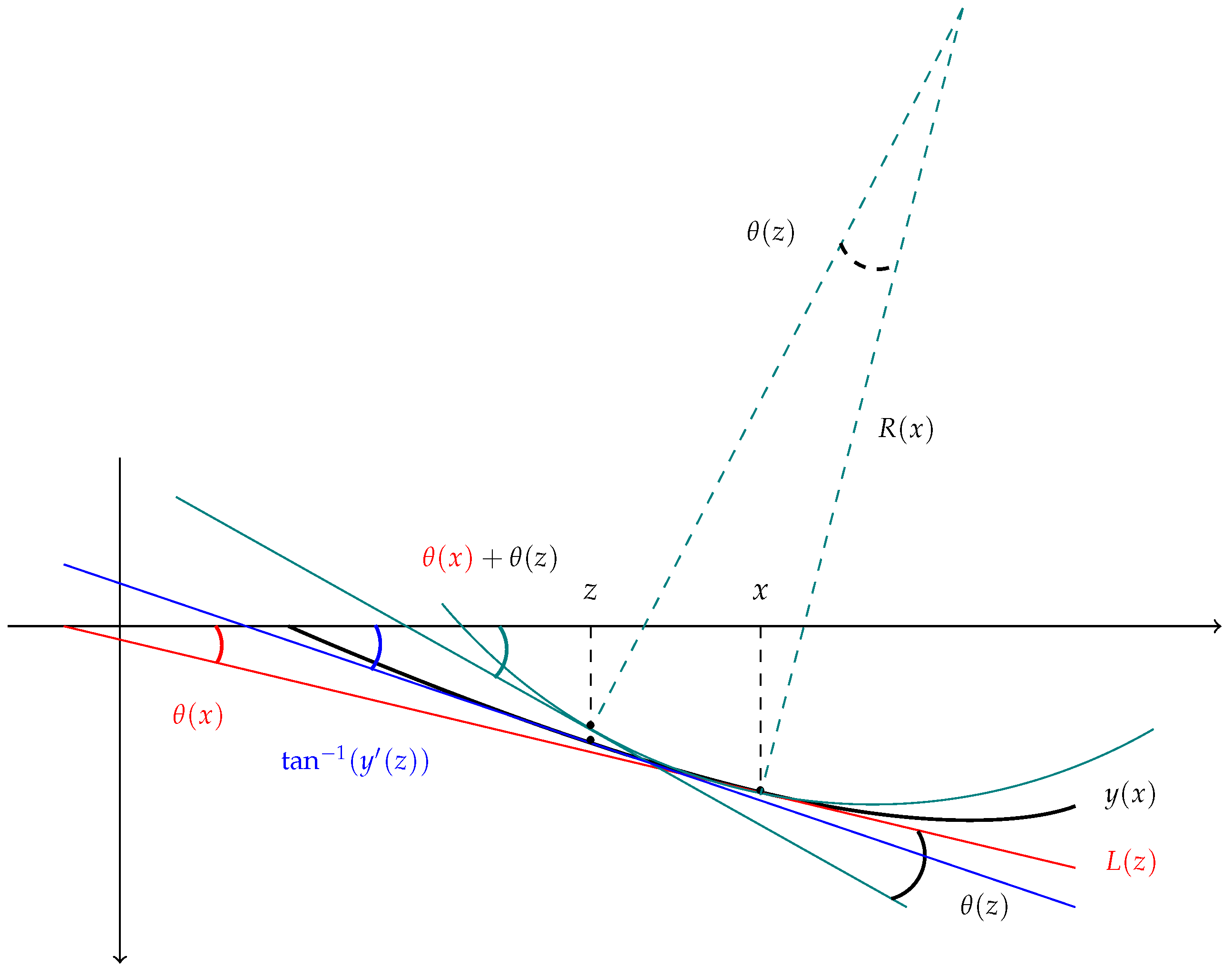
Indeed, it is clear that any stress or climatic change can affect the elastic curve of a beam. This macroscopic change is reflected in the radius of curvature. As it is well known, the usual deduction of radius of curvature uses differentials, which in the fractional context are not natural to introduce. In our case, we proceed with a different analysis. To fix the ideas, we consider the following scheme, see Figure 4.

Let $x\in (0,L)$ be an arbitrary fixed point and $\theta \left(x\right)\in (-\pi ,\pi )$ such that $y^{\prime }\left(x\right)=tan\theta \left(x\right)$, then

$$L\left(z\right)=y\left(x\right)+y^{\prime }\left(x\right)(z-x),z\in (0,L),$$

is the tangent line to the elastic curve y at the point $(x,y(x\left)\right)$. Let $\theta \left(z\right)$ be the increase in the angle (see Figure 4) by varying the variable z, to the left of x, $z<x$. We know that the length of the arc $S\left(z\right)$ corresponding to the circle of radius $R\left(x\right)$ and amplitude $\theta \left(z\right)$ is given by

$$S\left(z\right)=R\left(x\right)\theta \left(z\right),z\in (0,L).$$

(8)

In this case, $\theta \left(z\right)$ is negative since it rotates clockwise. We note that if z is close to x, then

$$S\left(z\right)\approx -\sqrt{{(z-x)}^2+{(L\left(z\right)-L\left(x\right))}^2}=-|z-x|\sqrt{1+{\left(y^{\prime }\left(x\right)\right)}^2}.$$

Using the linearity of the fractional derivative and Proposition 3, with $0<\alpha <1$, $n=1$ and $\beta =2$, we obtain

$$\begin{array}{ccc}\hfill D_{0+}^{\alpha }S\left(z\right)& \approx & -\sqrt{1+{\left(y^{\prime }\left(x\right)\right)}^2}{D}_{0+}^{\alpha }|z-x|\hfill \\ & =& \frac{\sqrt{1+{\left(y^{\prime }\left(x\right)\right)}^2}}{\mathsf{\Gamma }(2-\alpha )}·\left\{\begin{array}{cc}{z}^{1-\alpha },\hfill & 0<z<x,\hfill \\ z^{1-\alpha }-2{(z-x)}^{1-\alpha },\hfill & x<z<L.\hfill \end{array}\right.\hfill \end{array}$$

(9)

On the other hand, since $tanx\approx x$, for $\left|x\right|<\pi /2$, and assuming that the deflection in the beam is small (i.e., $\theta \left(x\right)\approx 0$), then

$$\theta \left(x\right)+\theta \left(z\right)\approx tan(\theta \left(x\right)+\theta \left(z\right))\approx y^{\prime }\left(z\right).$$

The fact that the fractional derivative of constant functions is zero and Proposition 2 yield

$$D_{0+}^{\alpha }\theta \left(z\right)=D_{0+}^{\alpha }(\theta \left(x\right)+\theta \left(z\right))\approx D_{0+}^{\alpha +1}y\left(z\right).$$

(10)

From (8), we have

$$D_{0+}^{\alpha }S\left(z\right){{|}_x=R\left(x\right)D_{0+}^{\alpha }\theta \left(z\right)|}_x.$$

As in the classical case, if we assume that the deflection is small, then the square of $y^{\prime }\left(x\right)$ is significantly less than 1, so using (9) and (10) we arrive at the approximation

$$R\left(x\right)\approx \frac{x^{1-\alpha }}{\mathsf{\Gamma }(2-\alpha )}·\frac{1}{D_{0+}^{\alpha +1}y\left(x\right)},$$

which has an extra factor compared to the classical approximation, see (4). Thus, using (7), we arrive at the fractional equation for the beam

$$EI{D}_{0+}^{\alpha +1}y\left(x\right)=\frac{x^{1-\alpha }}{\mathsf{\Gamma }(2-\alpha )}·M\left(x\right),x\in (0,L).$$

(11)

It is often found that, when dealing with models of real phenomena, see [6], in the fractional calculus, the classical derivatives are simply replaced by fractional derivatives, if this had been carried out, from (5) we would see that the resulting equation would be,

$$EI{D}_{0+}^{\alpha +1}y\left(x\right)=M\left(x\right),x\in (0,L).$$

In our case, an extra factor appears, $x^{1-\alpha }/\mathsf{\Gamma }(2-\alpha )$. In particular, for $0<\alpha <1$, the concavity of the function $x^{1-\alpha }$ means that small percentage values of x affect the bending moment $M\left(x\right)$ more. This intuitively means that if the index $\alpha$ represents in some sense the memory of the material (or an index of the climatic changes), then the most flexible part has the greatest opportunity to rearrange itself, and the opposite occurs in the most rigid parts, see the examples in Section 6.

Now, let us solve the Equation (11). Using Proposition 1 and the linearity of the Riemann–Liouville integral we arrive at

$$\begin{array}{ccc}\hfill EI\left(I_{0+}^{\alpha +1}{D}_{0+}^{\alpha +1}y\right)\left(x\right)& =& EI(y\left(x\right)-y\left(0\right)-y^{\prime }\left(0\right)x)\hfill \\ & =& \frac{1}{\mathsf{\Gamma }(2-\alpha )}{I}_{0+}^{\alpha +1}\left(x^{1-\alpha }M\left(x\right)\right),x\in (0,L).\hfill \end{array}$$

Consequently, the solution of the fractional differential Equation (11) is

$$y\left(x\right)=\frac{1}{EI\mathsf{\Gamma }(2-\alpha )}{I}_{0+}^{\alpha +1}\left(x^{1-\alpha }M\left(x\right)\right)+y^{\prime }\left(0\right)x+y\left(0\right),x\in (0,L).$$

(12)

In what follows, we will denote such function by $y_{\alpha }\left(x\right)$ and the classical solution as $y\left(x\right)$.

5. Some Analytical Examples

In this part, we will see some typical cases that occur in applications of suspended beams. In each case, we will first recall the solution $y\left(x\right)$ to the classical Equation (5) and then the solution $y_{\alpha }\left(x\right)$ to the fractional Equation (11). The examples that we present are generic, and in the next section we assign values to the parameters and we will comment on their solution.

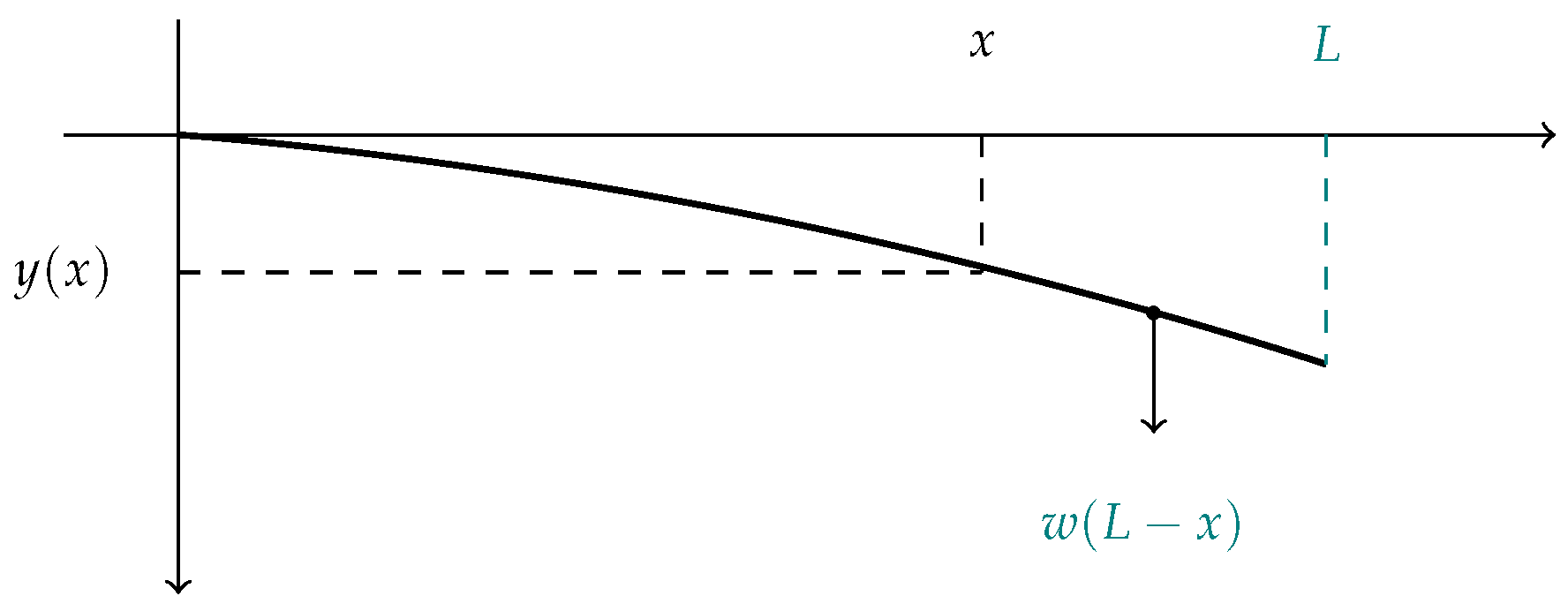
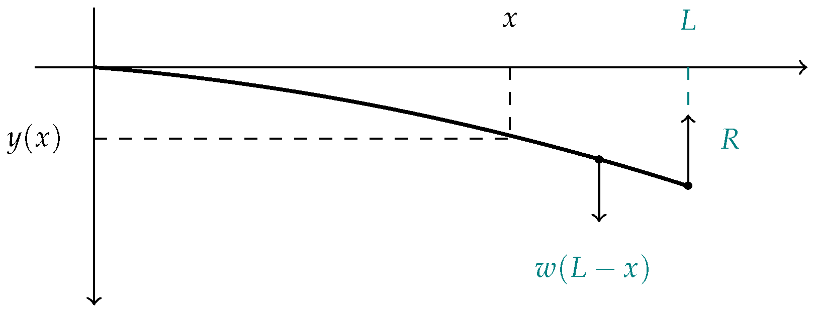
Example 1.

Let us suppose that our beam has one end fixed and the other is free, that is, it hangs. Suppose further that the weight of the beam is w and is uniformly distributed in the beam of length L. In this case, we have the scheme shown in Figure 5.

In this case, the bending moment is (see [23] for its deduction)

$$M\left(x\right)=\frac{w}{2}{(L-x)}^2,x\in (0,L).$$

Therefore, the elastic curve, in the classical case, will be

$$y\left(x\right)=\frac{w}{24EI}(x^4-4L{x}^3+6L^2{x}^2),x\in [0,L].$$

Consequently, the maximum deflection of the beam is given by

$$y\left(L\right)=\frac{w{L}^4}{8EI}.$$

Now, let us address the fractional case. The problem suggests that the initial conditions are $y_{\alpha }\left(0\right)=0$ and $y_{\alpha }^{\prime }\left(0\right)=0$, using (6) we see that the solution to (11) is given by

$$\begin{array}{ccc}\hfill y_{\alpha }\left(x\right)& =& \frac{1}{EI\mathsf{\Gamma }(2-\alpha )}{I}_{0+}^{\alpha +1}\left(x^{1-\alpha }\frac{w}{2}{(L-x)}^2\right)\hfill \\ & =& \frac{1}{EI\mathsf{\Gamma }(2-\alpha )}{I}_{0+}^{\alpha +1}\left(\frac{w{L}^2}{2}{x}^{1-\alpha }-wL{x}^{2-\alpha }+\frac{w}{2}{x}^{3-\alpha }\right)\hfill \\ & =& \frac{w}{48EI}\left[(3-\alpha )(2-\alpha )x^4-8(2-\alpha )L{x}^3+12L^2{x}^2\right].\hfill \end{array}$$

From which it follows that the maximum deflection is

$$y_{\alpha }\left(L\right)=\frac{w{L}^4}{48EI}(2+3\alpha +{\alpha }^2).$$

It is convenient to write these expressions in the form

$$y_{\alpha }\left(L\right)=c\left(\alpha \right)·y\left(L\right),\mathrm{where}c\left(\alpha \right)=\frac{1}{6}(2+3\alpha +{\alpha }^2).$$

(13)

Example 2.

Let us now consider a beam of length L where the left endpoint is fixed and at the right endpoint there is a force of magnitude R that opposes the deflection of the beam. Suppose further that the beam has a uniformly distributed weight w. With these data we have a scheme like the one in Figure 6.

Under these circumstances, the bending moment is given by (see [23])

$$M\left(x\right)=\frac{w}{2}{(L-x)}^2-R(L-x),x\in (0,L).$$

Therefore, the classical elastic curve is

$$y\left(x\right)=\frac{1}{24EI}\left[w{x}^4-4(wL-R)x^3-(12RL-6w{L}^2)x^2\right].$$

Let us consider now the fractional case. The initial conditions of this scheme are $y\left(0\right)=0$, $y^{\prime }\left(0\right)=0$. Therefore, using the linearity of the Riemann–Liouville integral and Proposition 3 we have that the elastic curve is (see the Equation (12))

$$y_{\alpha }\left(x\right)=\frac{1}{48EI}\left[w(3-\alpha )(2-\alpha )x^4-8(wL-R)(2-\alpha )x^3-\left(24RL-12w{L}^2\right)x^2\right].$$

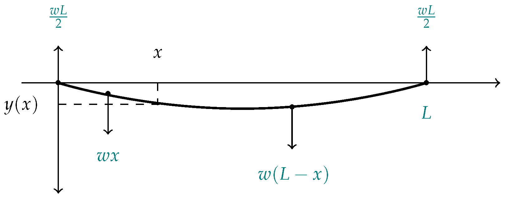
Example 3.

Suppose a beam of length L is simply supported at both ends. Furthermore, let us assume that the beam has a weight w uniformly distributed along the length of the beam by which it bends. In Figure 7, we show the corresponding scheme.

We know (see the [23]) that the bending moment is

$$M\left(x\right)=\frac{w}{2}{x}^2-\frac{wL}{2}x,$$

and that the classical elastic curve is given by

$$y\left(x\right)=\frac{w}{24EI}(x^4-2L{x}^3+L^{3}x).$$

From this, we see that the maximum deflection is at $L/2$ and is given by

$$y\left(\frac{L}{2}\right)=\frac{5w{L}^4}{384EI}.$$

We now turn to the fractional case. We begin by noting that if only one direction of the derivative is considered, that is, derivatives from the right $D_{-}^{\alpha }$ or derivatives from the left $D_{+}^{\alpha }$, then the solution of the resulting fractional differential equation is discontinuous, contrary to the continuity of the elastic curve. Because of this, the midpoint and a combination of fractional derivatives are considered. That is, in the interval $(0,L/2)$, we will use the fractional derivative from the right $D_{\frac{L}{2}-}^{\alpha }$, and in the interval $(L/2,L)$, we will consider the fractional left derivative $D_{\frac{L}{2}+}^{\alpha }$, denoting in each case the solution of the fractional equation by $y_{-}$ and $y_{+}$, respectively. From Formula (4) we obtain, proceeding as we did for the deduction of Equation (12),

$$\begin{array}{cc}\hfill & EI\left\{y_{-}\left(x\right)-y_{-}\left(\frac{L}{2}\right)+y_{-}^{\prime }\left(\frac{L}{2}\right)\left(\frac{L}{2}-x\right)\right\}\hfill \\ \hfill & =I_{\frac{L}{2}-}^{\alpha +1}\frac{{\left(\frac{L}{2}-x\right)}^{1-\alpha }}{\mathsf{\Gamma }(2-\alpha )}·\left(\frac{w}{2}{x}^2-\frac{wL}{2}x\right),0<x<\frac{L}{2},\hfill \\ \hfill & EI\left\{y_{+}\left(x\right)-y_{+}\left(\frac{L}{2}\right)-y_{+}^{\prime }\left(\frac{L}{2}\right)\left(x-\frac{L}{2}\right)\right\}\hfill \\ \hfill & =I_{\frac{L}{2}+}^{\alpha +1}\frac{{\left(x-\frac{L}{2}\right)}^{1-\alpha }}{\mathsf{\Gamma }(2-\alpha )}·\left(-\frac{w}{2}{x}^2-\frac{wL}{2}x\right),\frac{L}{2}<x<L.\hfill \end{array}$$

From Proposition 1 and the linearity of the fractional integral, we have

$$\begin{array}{cc}\hfill & \frac{1}{\mathsf{\Gamma }(2-\alpha )}{I}_{\frac{L}{2}-}^{\alpha +1}{\left(\frac{L}{2}-x\right)}^{1-\alpha }·\left(\frac{w}{2}{x}^2-\frac{wL}{2}x\right)\hfill \\ \hfill & =\frac{w}{2\mathsf{\Gamma }(2-\alpha )}{I}_{\frac{L}{2}-}^{\alpha +1}{\left(\frac{L}{2}-x\right)}^{3-\alpha }-\frac{w{L}^2}{8\mathsf{\Gamma }(2-\alpha )}{I}_{\frac{L}{2}-}^{\alpha +1}{\left(\frac{L}{2}-x\right)}^{1-\alpha }\hfill \\ \hfill & =\frac{w(3-\alpha )(2-\alpha )}{48}{\left(\frac{L}{2}-x\right)}^4-\frac{w{L}^2}{16}{\left(\frac{L}{2}-x\right)}^2,\hfill \end{array}$$

and

$$\begin{array}{cc}\hfill & \frac{1}{\mathsf{\Gamma }(2-\alpha )}{I}_{\frac{L}{2}+}^{\alpha +1}{\left(x-\frac{L}{2}\right)}^{1-\alpha }·\left(\frac{w}{2}{x}^2-\frac{wL}{2}x\right)\hfill \\ \hfill & =\frac{w}{2\mathsf{\Gamma }(2-\alpha )}{I}_{\frac{L}{2}+}^{\alpha +1}{\left(x-\frac{L}{2}\right)}^{3-\alpha }-\frac{w{L}^2}{8\mathsf{\Gamma }(2-\alpha )}{I}_{\frac{L}{2}+}^{\alpha +1}{\left(x-\frac{L}{2}\right)}^{1-\alpha }\hfill \\ \hfill & =\frac{w(3-\alpha )(2-\alpha )}{48}{\left(x-\frac{L}{2}\right)}^4-\frac{w{L}^2}{16}{\left(x-\frac{L}{2}\right)}^2.\hfill \end{array}$$

Using the value of these integrals in the previous expression, we obtain

$$\begin{array}{cc}\hfill & EI\left\{y_{-}\left(x\right)-y_{-}\left(\frac{L}{2}\right)+y_{-}^{\prime }\left(\frac{L}{2}\right)\left(\frac{L}{2}-x\right)\right\}\hfill \\ \hfill & =\frac{w(3-\alpha )(2-\alpha )}{48}{\left(\frac{L}{2}-x\right)}^4-\frac{w{L}^2}{16}{\left(\frac{L}{2}-x\right)}^2,0<x<\frac{L}{2},\hfill \\ \hfill & EI\left\{y_{+}\left(x\right)-y_{+}\left(\frac{L}{2}\right)-y_{+}^{\prime }\left(\frac{L}{2}\right)\left(x-\frac{L}{2}\right)\right\}\hfill \\ \hfill & =\frac{w(3-\alpha )(2-\alpha )}{48}{\left(x-\frac{L}{2}\right)}^4-\frac{w{L}^2}{16}{\left(x-\frac{L}{2}\right)}^2,\frac{L}{2}<x<L.\hfill \end{array}$$

The physical conditions of the problem tell us that the boundary conditions must be

$$y_{-}\left(0\right)=0,y_{+}\left(L\right)=0,$$

and the continuity conditions must be

$$y_{-}\left(\frac{L}{2}\right)=y_{+}\left(\frac{L}{2}\right),y_{-}^{\prime }\left(\frac{L}{2}\right)=y_{+}^{\prime }\left(\frac{L}{2}\right)=0.$$

This leads to

$$y_{-}^{\prime }\left(\frac{L}{2}\right)=\frac{1}{EI}·\left(\frac{w{L}^4}{64}-\frac{w{L}^4(3-\alpha )(2-\alpha )}{768}\right).$$

Consequently, the fractional elastic curve is given by

$$y_{\alpha }\left(x\right)=\frac{1}{16EI}·\left\{\begin{array}{cc}\frac{w{L}^4}{48}(6+5\alpha -{\alpha }^2)+\frac{w(3-\alpha )(2-\alpha )}{3}{\left(\frac{L}{2}-x\right)}^4-w{L}^2{\left(\frac{L}{2}-x\right)}^2,\hfill & 0\le x\le \frac{L}{2},\hfill \\ \frac{w{L}^4}{48}(6+5\alpha -{\alpha }^2)+\frac{w(3-\alpha )(2-\alpha )}{3}{\left(x-\frac{L}{2}\right)}^4-w{L}^2{\left(x-\frac{L}{2}\right)}^2,\hfill & \frac{L}{2}\le x\le L.\hfill \end{array}\right.$$

Which, of course, reflects the symmetry property of the elastic curve. From this, it follows that the value of the maximum deflection is

$$y_{\alpha }\left(\frac{L}{2}\right)=\frac{w{L}^4(6+5\alpha -{\alpha }^2)}{768EI},$$

therefore

$$y_{\alpha }\left(\frac{L}{2}\right)=c\left(\alpha \right)·y\left(\frac{L}{2}\right),\mathrm{where}c\left(\alpha \right)=\frac{6+5\alpha -{\alpha }^2}{10}.$$

(14)

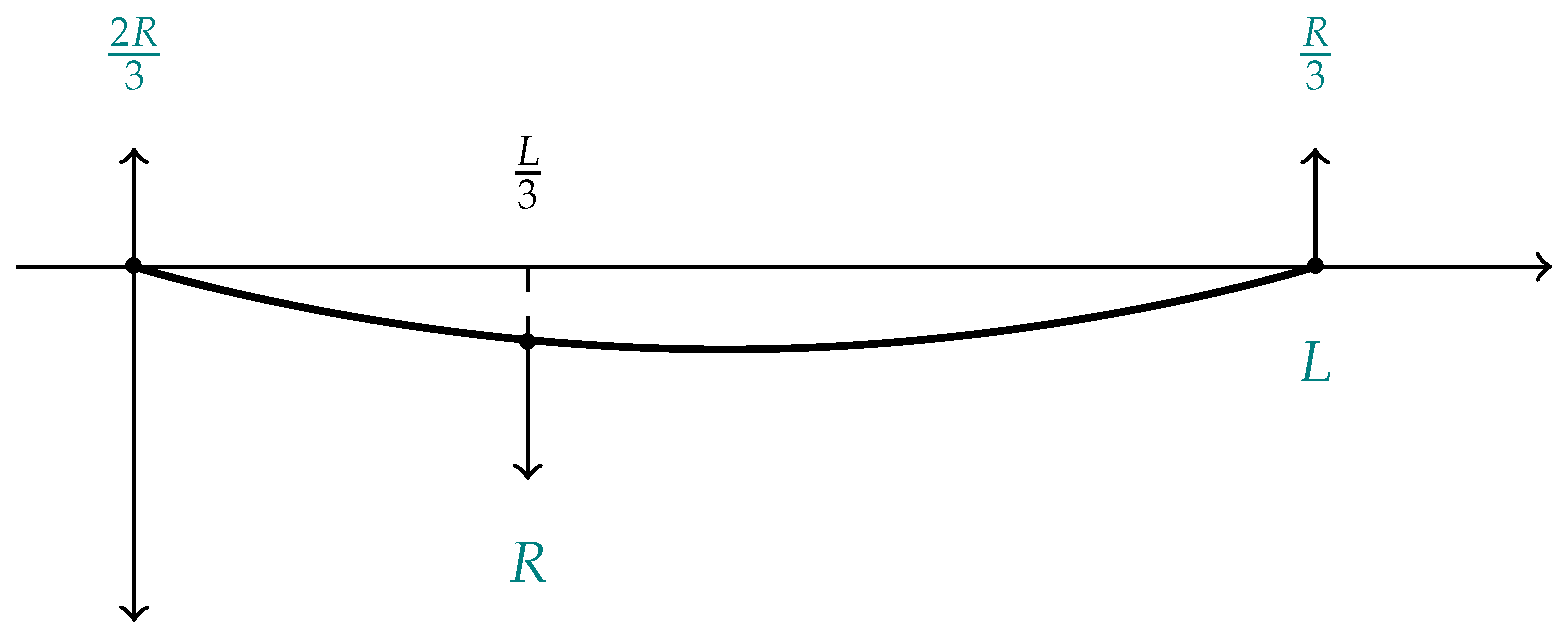
Example 4.

Consider a horizontal beam of length L and negligible weight that is simply supported at both ends. Let us further assume that the beam bends due to a load R concentrated at a distance $L/3$ from the left end. Under these data, we have the schema shown in Figure 8.

The bending moment is (see [23])

$$M\left(x\right)=\left\{\begin{array}{cc}-\frac{2R}{3}x,\hfill & 0<x<\frac{L}{3},\hfill \\ -\frac{RL}{3}+\frac{R}{3}x,\hfill & \frac{L}{3}<x<L.\hfill \end{array}\right.$$

Therefore, the elastic curve in the classical case is given by

$$y\left(x\right)=\frac{R}{81EI}·\left\{\begin{array}{cc}5L^{2}x-9x^3,\hfill & 0\le x\le \frac{L}{3}\hfill \\ \frac{9}{2}{x}^3-\frac{27}{2}L{x}^2+\frac{19}{2}{L}^{2}x-\frac{1}{2}{L}^3,\hfill & \frac{L}{3}\le x\le L,\hfill \end{array}\right.$$

with minimum point $\left(1-\frac{4}{\sqrt{54}}\right)L$ and minimum value

$$\frac{16\sqrt{2}}{729\sqrt{3}}·\frac{R{L}^3}{EI}.$$

(15)

Let us now turn to the fractional case. Similarly, to the previous case, in order to have a continuous solution it is necessary to start the fractional derivatives at an intermediate point of the interval $(0,L)$, in this case at $L/3$. Using (4), as the derivation of Equation (11), we arrive at the fractional equation

$$\begin{array}{ccc}\hfill EI{D}_{\frac{L}{3}-}^{\alpha +1}{y}_{-}\left(x\right)& =& \frac{{\left(\frac{L}{3}-x\right)}^{1-\alpha }}{\mathsf{\Gamma }(2-\alpha )}·\left(-\frac{2R}{3}x\right),0<x<\frac{L}{3},\hfill \end{array}$$

(16)

$$\begin{array}{ccc}\hfill EI{D}_{\frac{L}{3}+}^{\alpha +1}{y}_{+}\left(x\right)& =& \frac{{\left(x-\frac{L}{3}\right)}^{1-\alpha }}{\mathsf{\Gamma }(2-\alpha )}·\left(-\frac{RL}{3}+\frac{R}{3}x\right),\frac{L}{3}<x<L,\hfill \end{array}$$

(17)

where $y_{-}$ and $y_{+}$ represent the solution $y_{\alpha }$ on the intervals $(0,L/3)$ and $(L/3,L)$, respectively. Assuming the boundary conditions

$$y_{-}\left(0\right)=0,y_{+}\left(L\right)=0,$$

and furthermore, we assume the continuity of y and its derivative at $L/3$, that is,

$$y_{-}\left(\frac{L}{3}\right)=y_{+}\left(\frac{L}{3}\right),y_{-}^{\prime }\left(\frac{L}{3}\right)=y_{+}^{\prime }\left(\frac{L}{3}\right).$$

Using Proposition 1, together with the linearity of the fractional integral, we are left with

$$\begin{array}{ccc}\hfill EI{I}_{\frac{L}{3}-}^{\alpha +1}{D}_{\frac{L}{3}-}^{\alpha +1}{y}_{-}\left(x\right)& =& EI\left\{y_{-}\left(x\right)-y_{-}\left(\frac{L}{3}\right)+y_{-}^{\prime }\left(\frac{L}{3}\right)\left(\frac{L}{3}-x\right)\right\},0<x<\frac{L}{3},\hfill \\ \hfill EI{I}_{\frac{L}{3}+}^{\alpha +1}{D}_{\frac{L}{3}+}^{\alpha +1}{y}_{+}\left(x\right)& =& EI\left\{y_{+}\left(x\right)-y_{+}\left(\frac{L}{3}\right)-y_{+}^{\prime }\left(\frac{L}{3}\right)\left(x-\frac{L}{3}\right)\right\},\frac{L}{3}<x<L.\hfill \end{array}$$

On the other hand, using Proposition 3, we obtain

$$\begin{array}{cc}\hfill & I_{\frac{L}{3}-}^{\alpha +1}\frac{{\left(\frac{L}{3}-x\right)}^{1-\alpha }}{\mathsf{\Gamma }(2-\alpha )}·\left(-\frac{2R}{3}x\right)\hfill \\ \hfill & =-\frac{2R}{3\mathsf{\Gamma }(2-\alpha )}{I}_{\frac{L}{3}-}^{\alpha +1}{\left(\frac{L}{3}-x\right)}^{1-\alpha }x\hfill \\ \hfill & =\frac{2R}{3\mathsf{\Gamma }(2-\alpha )}{I}_{\frac{L}{3}-}^{\alpha +1}{\left(\frac{L}{3}-x\right)}^{2-\alpha }-\frac{2RL}{9\mathsf{\Gamma }(2-\alpha )}{I}_{\frac{L}{3}-}^{\alpha +1}{\left(\frac{L}{3}-x\right)}^{1-\alpha }\hfill \\ \hfill & =\frac{R(2-\alpha )}{9}{\left(\frac{L}{3}-x\right)}^3-\frac{RL}{9}{\left(\frac{L}{3}-x\right)}^2,\hfill \end{array}$$

and

$$\begin{array}{cc}\hfill & I_{\frac{L}{3}+}^{\alpha +1}\frac{{\left(x-\frac{L}{3}\right)}^{1-\alpha }}{\mathsf{\Gamma }(2-\alpha )}·\left(-\frac{RL}{3}+\frac{R}{3}x\right)\hfill \\ \hfill & =-\frac{2RL}{9\mathsf{\Gamma }(2-\alpha )}{I}_{\frac{L}{3}+}^{\alpha +1}{\left(\frac{L}{3}-x\right)}^{1-\alpha }+\frac{R}{3\mathsf{\Gamma }(2-\alpha )}{I}_{\frac{L}{3}+}^{\alpha +1}{\left(\frac{L}{3}-x\right)}^{2-\alpha }\hfill \\ \hfill & =-\frac{RL}{9}{\left(x-\frac{L}{3}\right)}^2+\frac{R(2-\alpha )}{18}{\left(x-\frac{L}{3}\right)}^3.\hfill \end{array}$$

Thus, we arrive at the equation

$$\begin{array}{cc}\hfill & EI\left\{y_{-}\left(x\right)-y_{-}\left(\frac{L}{3}\right)+y_{-}^{\prime }\left(\frac{L}{3}\right)\left(\frac{L}{3}-x\right)\right\}\hfill \\ \hfill & =\frac{R(2-\alpha )}{9}{\left(\frac{L}{3}-x\right)}^3-\frac{RL}{9}{\left(\frac{L}{3}-x\right)}^2,0<x<\frac{L}{3},\hfill \\ \hfill & EI\left\{y_{+}\left(x\right)-y_{+}\left(\frac{L}{3}\right)-y_{+}^{\prime }\left(\frac{L}{3}\right)\left(x-\frac{L}{3}\right)\right\}\hfill \\ \hfill & =-\frac{RL}{9}{\left(x-\frac{L}{3}\right)}^2+\frac{R(2-\alpha )}{18}{\left(x-\frac{L}{3}\right)}^3,\frac{L}{3}<x<L.\hfill \end{array}$$

From the boundary and continuity conditions, we obtain the system of equations

$$\begin{array}{ccc}\hfill EI\left\{-y_{\alpha }\left(\frac{L}{3}\right)+y_{\alpha }^{\prime }\left(\frac{L}{3}\right)·\frac{L}{3}\right\}& =& \frac{R(2-\alpha )}{9}{\left(\frac{L}{3}\right)}^3-\frac{RL}{9}{\left(\frac{L}{3}\right)}^2,\hfill \\ \hfill EI\left\{-y_{\alpha }\left(\frac{L}{3}\right)-y_{\alpha }^{\prime }\left(\frac{L}{3}\right)·\frac{2L}{3}\right\}& =& -\frac{RL}{9}{\left(\frac{2L}{3}\right)}^2+\frac{R(2-\alpha )}{18}{\left(\frac{2L}{3}\right)}^3,\hfill \end{array}$$

which has the solution

$$y_{\alpha }\left(\frac{L}{3}\right)=\frac{2R{L}^3}{243EI}(1+\alpha ),y_{\alpha }^{\prime }\left(\frac{L}{3}\right)=\frac{R{L}^2}{281EI}(1+\alpha ).$$

Putting this information together, we arrive at the solution of Equations (16) and ()

$$y_{\alpha }\left(x\right)=\frac{R}{EI}·\left\{\begin{array}{cc}\frac{2L^3(1+\alpha )}{243}-\frac{L^2(1+\alpha )}{81}\left(\frac{L}{3}-x\right)-\frac{L}{9}{\left(\frac{L}{3}-x\right)}^2+\frac{(2-\alpha )}{9}{\left(\frac{L}{3}-x\right)}^3,\hfill & 0\le x\le \frac{L}{3},\hfill \\ \frac{2L^3(1+\alpha )}{243}+\frac{L^2(1+\alpha )}{81}\left(x-\frac{L}{3}\right)-\frac{L}{9}{\left(x-\frac{L}{3}\right)}^2+\frac{(2-\alpha )}{18}{\left(x-\frac{L}{3}\right)}^3,\hfill & \frac{L}{3}\le x\le L.\hfill \end{array}\right.$$

(18)

To determine the maximum deflection of the beam we note that the points

$$\left(1-\frac{\sqrt{3}-\sqrt{5+\alpha -{\alpha }^2}}{\sqrt{3}(2-\alpha )}\right)\frac{L}{3},\left(1+\frac{2\left(\sqrt{6}-\sqrt{4-\alpha +{\alpha }^2}\right)}{\sqrt{6}(2-\alpha )}\right)\frac{L}{3}$$

are the critical points of $y_{\alpha }$. Since $\sqrt{3}<\sqrt{5+\alpha -{\alpha }^2}$, then $y_{-}$ is increasing on the interval $(0,L/3)$, which means that its maximum will be $y_{-}(L/3)=y_{+}(L/3)$. On the other hand, since

$$\frac{2\left(\sqrt{6}-\sqrt{4-\alpha +{\alpha }^2}\right)}{\sqrt{6}(2-\alpha )}<1,$$

then the maximum of $y_{+}$ in the interval $(L/3,L)$ will be reached in

$$\left(1+\frac{2\left(\sqrt{6}-\sqrt{4-\alpha +{\alpha }^2}\right)}{\sqrt{6}(2-\alpha )}\right)\frac{L}{3}.$$

From which it follows that the maximum of $y_{\alpha }$ in $(0,L)$ is

$$\frac{16\sqrt{2}R{L}^3}{729\sqrt{3}EI}·c\left(\alpha \right),$$

where

$$\begin{array}{cc}\hfill & c\left(\alpha \right)=\frac{3\sqrt{3}}{16\sqrt{2}}\left\{2(1+\alpha )\left(1+\frac{\sqrt{6}-\sqrt{4-\alpha +{\alpha }^2}}{\sqrt{6}(2-\alpha )}\right)\right.\hfill \\ \hfill & \left.+\frac{2{(\sqrt{6}-\sqrt{4-\alpha +{\alpha }^2})}^2}{3{(2-\alpha )}^2}\left(\frac{\sqrt{6}-\sqrt{4-\alpha +{\alpha }^2}}{\sqrt{6}}-3\right)\right\}.\hfill \end{array}$$

(19)

Therefore

The maximum deflection of $y_{\alpha }=c\left(\alpha \right)·$ The maximum deflection of y.

6. Some Numerical Examples

In this section, we consider the previous examples for some specific values of the parameters. Additionally, we will discuss the meaning of the fractional index for each case. Next, we will assume that the flexural stiffness $EI$ is the constant one and that the length of the beam is one. In symbols, $EI=1$ and $L=1$. The fractional parameter $\alpha$ will be in $[0,1]$. It should be noted that in the graphs of the following examples, the scale of the ordinates is different from the scale of the abscissas, this helps to appreciate the effect of deflection of the beam.

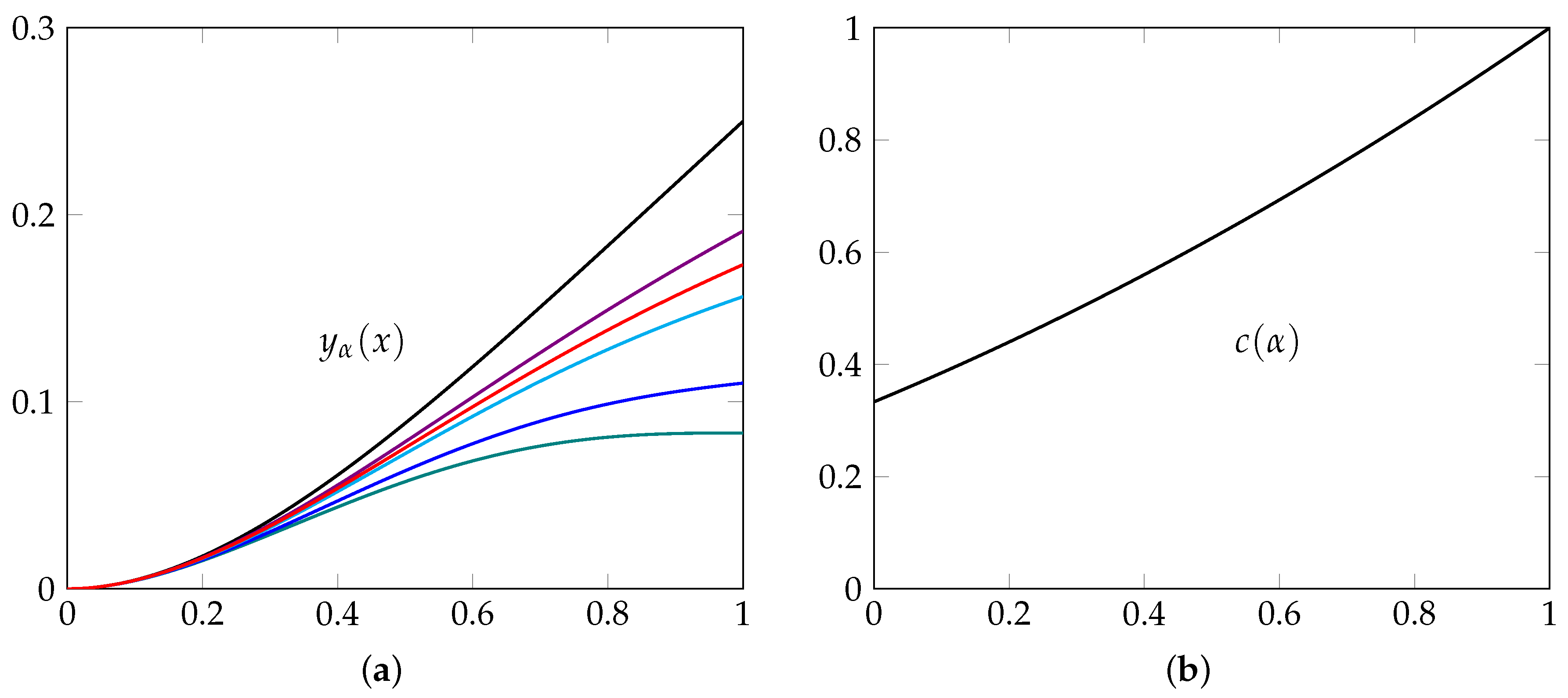
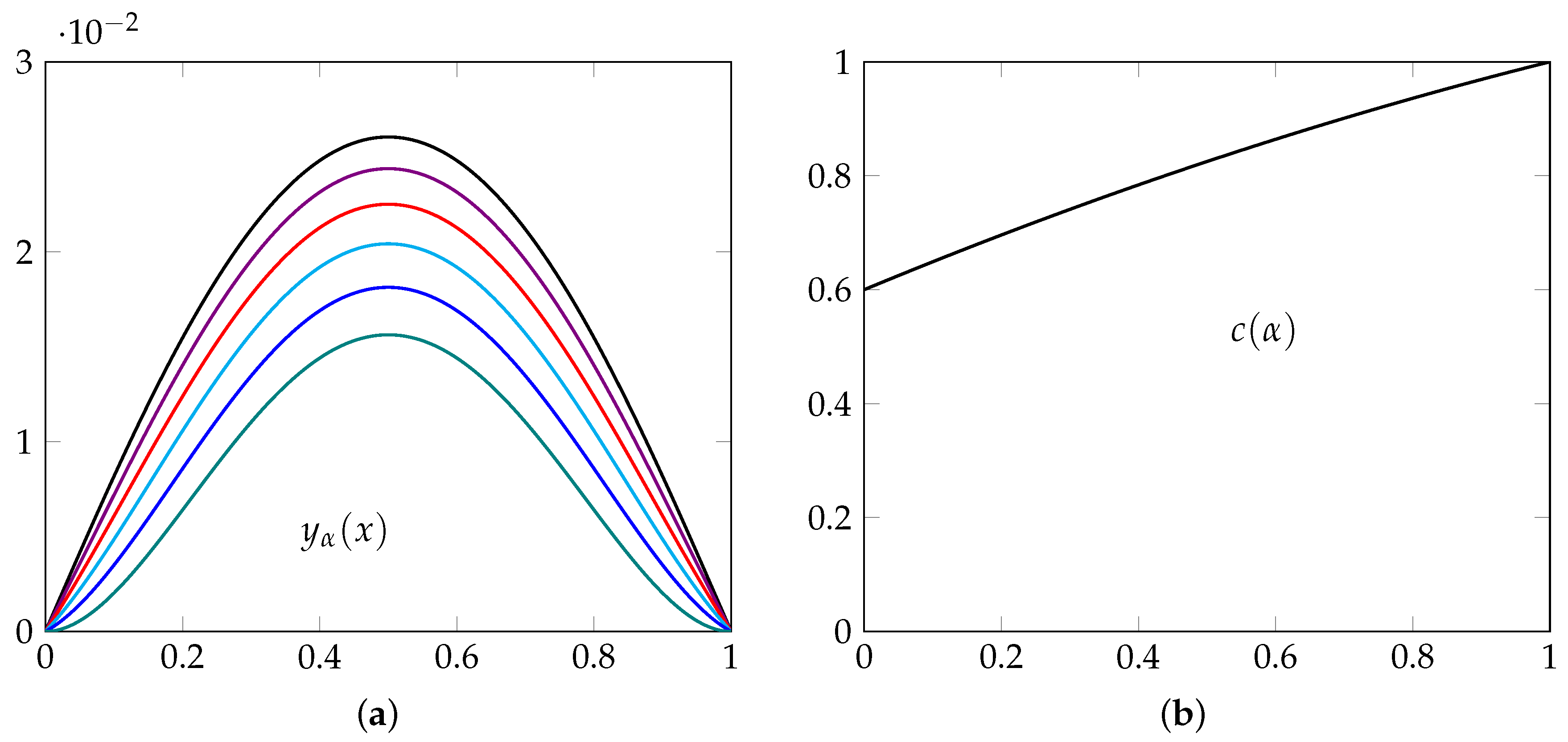
Example 5.

Let us suppose that $w=2$. The elastic curve in the classic case is

$$y\left(x\right)=\frac{1}{12}(x^4-4x^3+6x^2),x\in [0,1],$$

and in the fractional case is

$$y_{\alpha }\left(x\right)=\frac{1}{24}\left[(3-\alpha )(2-\alpha )x^4-8(2-\alpha )x^3+12x^2\right],x\in [0,1].$$

(20)

In Figure 9a we present the graph of the classical solution and the fractional solution, for several values of parameter $\alpha$. On the other hand, the graph of the function $c\left(\alpha \right)$, given in (13), appears in Figure 9b.

From Figure 9a, we appreciate that the fractional index $\alpha$ can help us to model the behavior of hanging beams in which there is a certain type of stiffness, for $0<\alpha <1$. This fact is corroborated by the graph that appears in Figure 9b, since the factor $c\left(\alpha \right)$ is always less than one, see the expression (13). The stiffening effect on the beam could be due either to changes in the material over time or due to some sensitivity to climatic changes. Furthermore, from Figure 9a, we notice that the values of the parameter $\alpha$ close to 0 describe a very different behavior from those close to one. Those that are close to 0 give us the impression that the beam is not completely homogeneous and could be used to model beams of non-homogeneous material, such as the case of wooden beams, which are commonly used in some countries, as the United States of America (USA). From Figure 9b, we also wee see that for $\alpha$ a little bigger than 1 we have an elastic effect in the beam.

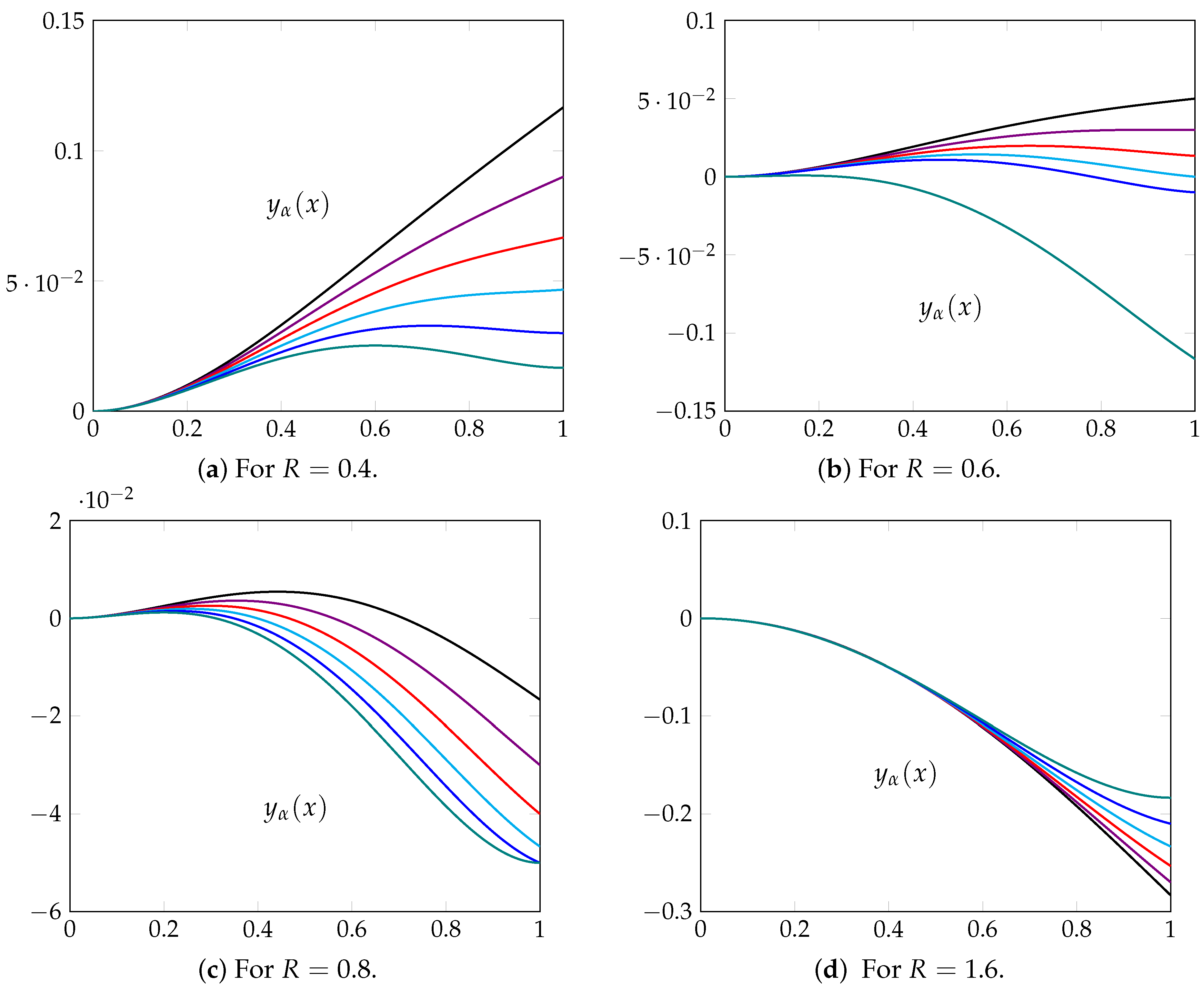
Example 6.

Here, we will assume that $w=2$. So, the elastic curve in the classical case is

$$y\left(x\right)=\frac{1}{12}\left[x^4-2(2-R)x^3-6(R-1)x^2\right],x\in [0,1],$$

and in the fractional case it is

$$y_{\alpha }\left(x\right)=\frac{1}{24}\left[(3-\alpha )(2-\alpha )x^4-4(2-R)(2-\alpha )x^3-12\left(R-1\right)x^2\right],x\in [0,1].$$

(21)

In Figure 10, we present the graph of the function $y_{\alpha }$ for various values of the parameters R and $\alpha$.

In this part, of course, the effect that the force R has on the deflection of the beam is observed. When the force is moderately small, $R=0.4$, see Figure 10a, and the fractional indices $\alpha$ are close to one, no buckling of the beam is observed. However, for $\alpha$ close to zero, the opposite happens. In fact, when $\alpha =0$, it is observed that there is an inflection point of the elastic curve. When R increases a bit, to $R=0.6$, see Figure 10b, then it almost equals the deflection force produced by the weight on the right side. Here we notice that there is a drastic change in the behavior of the elastic curve when the values of the fractional index are close to zero and one, respectively. This difference starts to be noticeable when $\alpha =0.2$ and then speeds up rapidly. In the case of $R=0.8$, see Figure 10c, that is, the force is medium, so the opposite effect occurs. Which means, in the classic case, a notorious buckling of the beam is observed and it becomes lighter when the fractional index decreases. In this case, it should be noted that for $\alpha =0$ a concavity change is observed at the end of the right end, which can indicate a variation in the homogeneity of the beam and that the central part is more flexible than the ends. Finally, in Figure 10d a force relatively greater than the previous ones is considered, $R=1.6$, and here, as expected, the elastic curve does not change concavity, except when the fractional index is very close to zero. In this case, it is observed that the fractional index can model the bending of beams in which they become more rigid due to the passage of time or due to climatic changes. From this example, we learn that if the force R causes the beam to have no deflection, then the behavior of $\alpha$ close to one and zero are very different, indicating an opportunity for the fractional model when working with beams where it is assumed that the climatic effect may be an important factor to consider in the model.

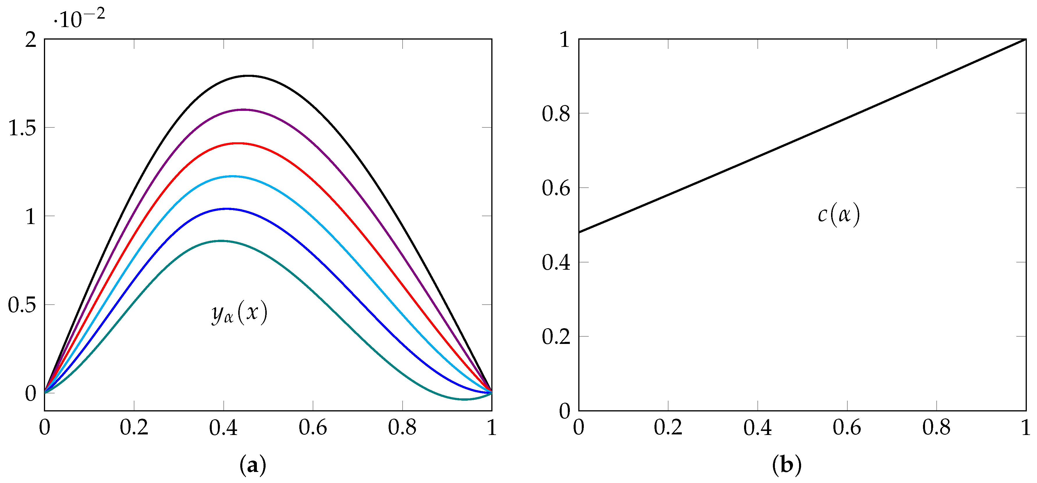
Example 7.

We will assume that $w=2$. With these data, the classical solution of Equation (5) is

$$y\left(x\right)=\frac{1}{12}(x^4-2x^3+x),$$

and the solution of the fractional Equation (11) is

$$y_{\alpha }\left(x\right)=\frac{1}{16}·\left\{\begin{array}{cc}\frac{1}{24}(6+5\alpha -{\alpha }^2)+\frac{2(3-\alpha )(2-\alpha )}{3}{\left(\frac{1}{2}-x\right)}^4-2{\left(\frac{1}{2}-x\right)}^2,\hfill & 0\le x\le \frac{1}{2},\hfill \\ \frac{1}{24}(6+5\alpha -{\alpha }^2)+\frac{2(3-\alpha )(2-\alpha )}{3}{\left(x-\frac{1}{2}\right)}^4-2{\left(x-\frac{1}{2}\right)}^2,\hfill & \frac{1}{2}\le x\le 1.\hfill \end{array}\right.$$

(22)

From Figure 11, we deduce that the fractional index $\alpha$ represents a measure of the stiffness of the beam. Indeed, in Figure 11b, we see that the maximum length of the beam decreases as $\alpha$ approaches 0. Furthermore, when $\alpha$ is approximately 0, a slight change in concavity can be seen at the ends, indicating that there is a certain variation in the homogeneity of the material at the ends, which makes the beam more rigid, see Figure 11a. On the other hand, the same figure indicates that the fractional index is related to the stiffness of the beam when $0<\alpha <1$ and effect of flexibility for $\alpha >1$. This may be justified if the construction material of the beam is sensitive to climatic changes, such as certain plastic or metal alloys, as we have said before.

Example 8.

We consider here the corresponding numerical version of Example 4 given in the previous section. For this example, the classical elastic curve is

$$y\left(x\right)=\frac{R}{81}·\left\{\begin{array}{cc}5x-9x^3,\hfill & 0\le x\le \frac{1}{3},\hfill \\ \frac{9}{2}{x}^3-\frac{27}{2}{x}^2+\frac{19}{2}x-\frac{1}{2},\hfill & \frac{1}{3}\le x\le 1,\hfill \end{array}\right.$$

and the fractional curve is

$$y_{\alpha }\left(x\right)=R·\left\{\begin{array}{cc}\frac{2(1+\alpha )}{243}-\frac{(1+\alpha )}{81}\left(\frac{1}{3}-x\right)-\frac{1}{9}{\left(\frac{1}{3}-x\right)}^2+\frac{(2-\alpha )}{9}{\left(\frac{1}{3}-x\right)}^3,\hfill & 0\le x\le \frac{1}{3},\hfill \\ \frac{2(1+\alpha )}{243}+\frac{(1+\alpha )}{81}\left(x-\frac{1}{3}\right)-\frac{1}{9}{\left(x-\frac{1}{3}\right)}^2+\frac{(2-\alpha )}{18}{\left(x-\frac{1}{3}\right)}^3,\hfill & \frac{1}{3}\le x\le 1.\hfill \end{array}\right.$$

(23)

Since the force R has a multiplicative effect on the elastic curve, it is enough to consider $R=1$.

From Figure 12a, we note that the fractional index can help us, in this case, to model deflection of beams in which there is a certain effect of stiffness, for $0<\alpha <1$, especially the fractional model can be important when the index $\alpha$ is greater than $0.5$. On the other hand, for values close to 0, a strong effect of non-homogeneity of the material is observed. Even a slight change in slope is observed when $\alpha$ is 0. Furthermore, from Figure 12b, we see that the maximum curvature decreases proportionally as the parameter $\alpha$ varies, reinforcing the stiffness or deflection phenomenon.

7. Discussion

In this part, we will comment the results obtained. First of all, let us notice that we use an approximation of the arc of the osculating circle to derive a fractional differential equation. This led us to consider a fractional differential equation in which an extra term appears, if only the classical derivative had been replaced by a fractional derivative. It seems to us that this way of avoiding the use of fractional differentials has a fairly wide potential and useful consequences in mathematical modeling, both theoretical and practical. In general, we observe that when the fractional index is close to zero, the model obtained is radically different from when the index is close to one. In this case, the assumption of homogeneity of the beam is broken. On the other hand, when the fractional index is close to one, we see that the classical solution is greater than the fractional solution. This observation is very important because it indicates that the beam acquires rigidity, which may be due to the environment that surrounds it. So, the fractional index indicates a measure of the stiffness of the beam. It should be noted that if in the solutions of the fractional equations of the examples if we consider the fractional parameter greater than one, then an opposite effect occurs, that is, in this case the fractional solution is always greater than the classical solution, showing that there is a dilation effect on the beam.