Optimization, Control, and Design of Arbitrarily Shaped Fan Arrays

Abstract

In many air conditioning applications fan arrays offer an increasingly popular alternative to single large fans due to redundancy and ease of maintainability. Additionally, there is the possibility to dynamically resize the array by selectively turning off a number of fans. In this work, a new method for the optimal control of such fan arrays is derived with the goal to minimize the overall power consumption, i.e., maximizing the system efficiency. The approach is universal in the sense that a fan array can be composed of any number, size, and type of fans or mixtures thereof. We explore the achievable power savings for a real world example by applying the method. Moreover, we give an outline of the optimal design of fan arrays and future work.

1. Introduction

Although the aerodynamic efficiency of single fans still rises through further development, the research and development in the field of fan systems will get even more important in the future. Nowadays, medium to large-sized fans in traditional applications are increasingly replaced by fan arrays; that is, a number of usually smaller fans operating in parallel. This is due to a number of generally accepted advantages. One obvious benefit is the redundancy of fans. If there is a failure of a single fan in the fan array, the remaining fans can partially or completely compensate by managing their operating speed appropriately. Along with this goes the ease for replacement of smaller-sized fans as compared to one large device. On the other hand, there are also application-specific profits. In a heat exchanger application, for example, it can be shown that the use of fan arrays leads to a significantly lower pressure loss and higher convective heat transfer, because of the more even flow profile over the heat exchanger as compared to a more uneven profile generated by a large single fan [1]. In addition to the aforementioned advantages, fan arrays offer additional degrees of freedom [2]. In applications with varying operating points, large improvement in system efficiency and high energy savings can be archived [3]. This is achieved by selectively turning off some of the fans in an array while controlling the operation of the remaining active fans accordingly. For this purpose we propose a method for the optimal control of such fan arrays [4]. In our approach, the arrays can be composed of an arbitrary number of different-sized fans and/or fans with different fan curve characteristics.

The paper is organized as follows: In the first section, we will introduce the necessary physical quantities involved in the operation of a fan array and derive our method for optimal control of such arrays. In the second section, we will apply the proposed method to a real-world problem to demonstrate the achievable system performance improvements. Finally, we give an outline for the optimal design of fan arrays and conclude our findings.

2. Method Description

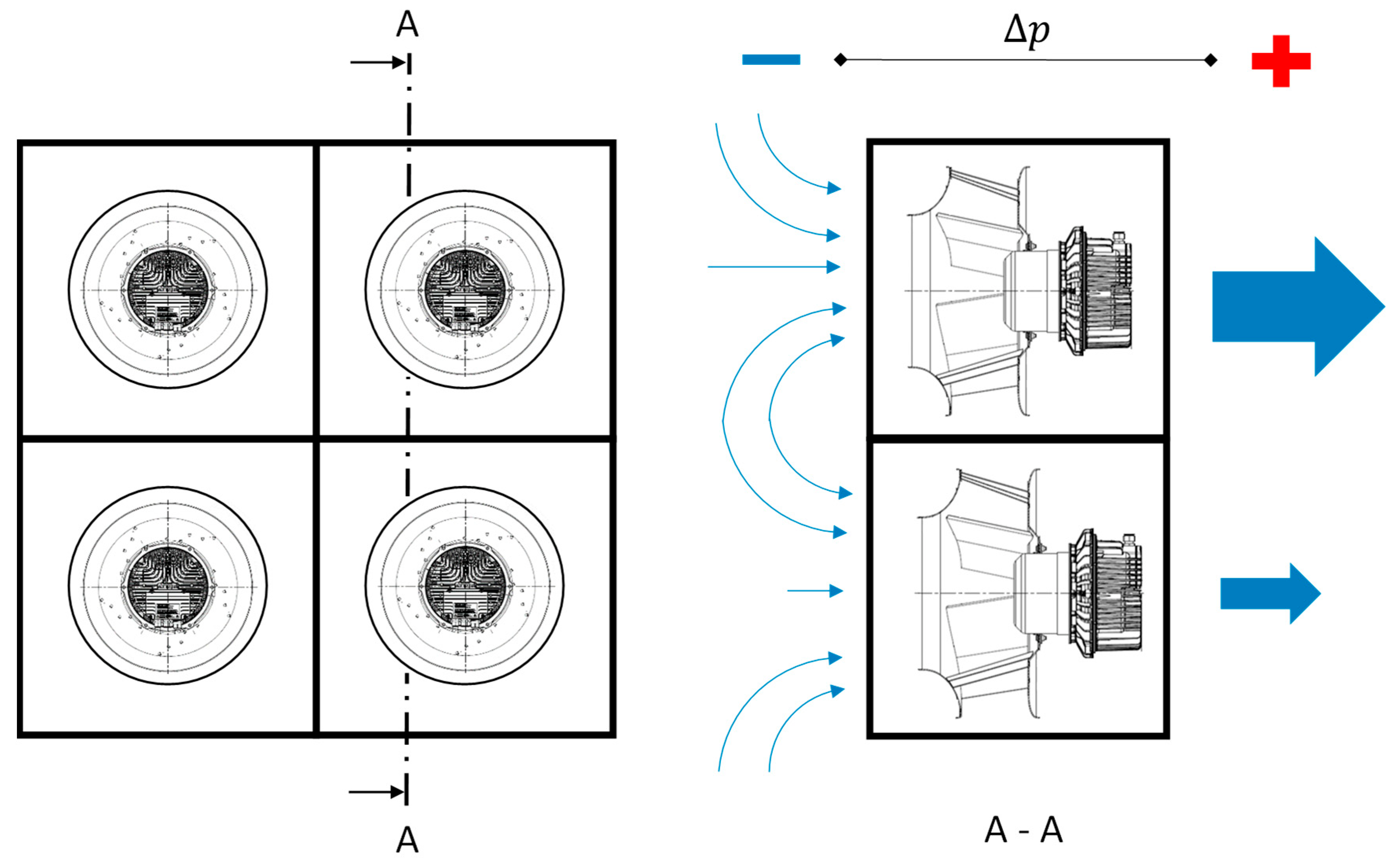
The A fan array of size $k_{max}$ is defined as $k_{max}$ (not necessarily identical) fans operating in parallel. That is, all fans in the array deliver the same static pressure rise. However, depending on their individual speed, their individual contribution to the overall volume flow rate might be different. This is depicted schematically in Figure 1 with four ebm-papst R3G500 centrifugal fans in a 2 × 2 setup.

There are only two prerequisites present in the theoretical derivation of our method:

• It is assumed that the speed of each fan in the array of fans can be variably controlled up to its maximum rotational speed;
• It is assumed that no backflow occurs in situations where fans are turned off. In reality, this can be achieved using, i.e., some kind of shutters or backdraft dampers.

The non-dimensional fan power for each individual fan in the array, denoted by index i, is given by:

$$P_i^{*}=\frac{{\psi }_i·{\phi }_i}{{\eta }_i},$$

(1)

with the well known pressure number $\psi ,$ flow number $\phi$, and the efficiency $\eta$. The dimensional power is thus given by:

$$P_i=P_i^{*}·\frac{{\pi }^4·D_i^5·n_i^3·\rho }{8},$$

(2)

with diameter D and operating speed n of the i-th fan in the array and density ρ.

2.1. Fixed Array Size with identical Fans

Now, we consider the fan array with a fixed number $k_{max}$ and fixed type of fans. That is, in the following, the $D_i$ are set to a constant value and the operating speeds $n_i$ become the sole free variables in the system. The goal of our method is to find the optimal speed for each individual fan.

The optimality condition for an array with size k and given operating point $\mathsf{\Delta }p$ and $Q_{tot}$ is the minimization of the total power consumption of the array:

$$\begin{gathered} \min \text{:} P_{tot}^{}={{\displaystyle \sum }}_{i=1}^k{P}_i^{}\left(n_i\right), \\ \mathrm{Subject} \mathrm{to}\text{:}{Q}_{tot}={{\displaystyle \sum }}_{i=1}^k{Q}_i\left(n_i\right) , \end{gathered}$$

where $Q_i={\phi }_i·{\pi }^2·D_i^3·n_i/4$ is the volume flow rate for the i-th individual fan in the array. As this is a continuous non-linear programming problem (NLP) with a single equality constraint, we choose the method of Lagrange multipliers for its solution [5]. This formulation of the optimization problem leads to a non-linear system of equations with $k+1$ unknowns (k speeds plus one Lagrange multiplier λ for the volume flow rate constraint):

$$\begin{gathered} \frac{\partial P_1^{}}{\partial n_1}=\lambda ·\frac{\partial Q_1}{\partial n_1} \\ ⋮ \\ \frac{\partial P_k^{}}{\partial n_k}=\lambda ·\frac{\partial Q_k}{\partial n_k} \\ {Q}_{tot}={\displaystyle \sum }_{i=1}^k{Q}_i\left(n_i\right) \end{gathered}$$

(3)

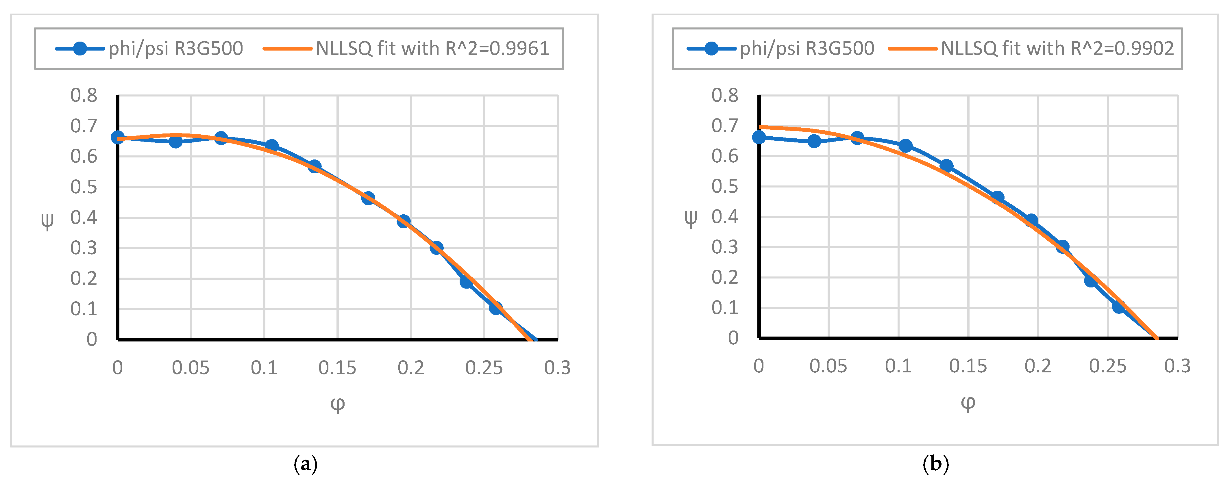
For the solution of this system of equations, the partial derivatives of the dimensional power with respect to the operating speed are required. In order to make the optimization problem accessible to a calculation, the power and the volume flow rate are transformed in such a way that they are pure functions of the speed. At this point, the dimensionless pressure and efficiency curves of the fans used in an array are introduced. In the following, we stick to the special case of an ebmpapst R3G500 centrifugal fan characteristic shown in Figure 2. However, this is for demonstration purposes and does not restrict the validity of our approach. The overall shape of the performance and efficiency characteristic curves will always be similar for all conventional fans due to well-known loss mechanisms [6,7].

From Equation (3) it is obvious that we need to approximate the fan characteristics using continuously differentiable functions. The respective dimensionless pressure characteristic of a fan is approximated with a second-order polynomial Equation (4). Preference is given here to the approximation with a quadratic approach Equation (5), since the approximation function is then strictly monotonic in the considered range $\phi$ > 0. This is an idealization because in reality, the fan stalls for low $\phi$ and the operation becomes unstable. One would have to define a minimum $\phi$, but we opt for this approach to demonstrate the method.

$${\psi }_i\left({\phi }_i\right)=a_{\psi ,i}·{\phi }_i^2+b_{\psi ,i}·{\phi }_i+c_{\psi ,i}$$

(4)

$${\psi }_i\left({\phi }_i\right)=a_{\psi ,i}·{\phi }_i^2+c_{\psi ,i}$$

(5)

With this description of the pressure number, the flow number can be expressed as a function of the constant coefficients of the polynomial approximation, diameter, density, speed, and pressure increase. Resolving the quadratic Equation (4) for the flow number yields:

$${\phi }_i\left(n_i\right)=-\frac{b_{\psi ,i}}{2a_{\psi ,i}}+\sqrt{{\left(\frac{b_{\psi ,i}}{2a_{\psi ,i}}\right)}^2-\frac{c_{\psi ,i}}{a_{\psi ,i}}+\frac{2\mathsf{\Delta }p}{\rho ·{\pi }^2·D_i^2·n_i^2·a_{\psi ,i}}}.$$

(6)

The derivative of the flow number with respect to the fan speed is given by:

$$\frac{\partial {\phi }_i}{\partial n_i}=-\frac{\frac{2\mathsf{\Delta }p}{\rho ·{\pi }^2·D_i^2·n_i^3·a_{\psi ,i} }}{\sqrt{{\left(\frac{b_{\psi ,i}}{2a_{\psi ,i}}\right)}^2-\frac{c_{\psi ,i}}{a_{\psi ,i}}+\frac{2\mathsf{\Delta }p}{\rho ·{\pi }^2·D_i^2·n_i^2·a_{\psi ,i}}}} .$$

(7)

Accordingly, the efficiency characteristics need to be approximated. Preference is given here to a fourth order polynomial:

$${\eta }_i\left({\phi }_i\right)=a_{\eta ,i}·{\phi }_i^4+b_{\eta ,i}·{\phi }_i^3+c_{\eta ,i}·{\phi }_i^2+d_{\eta ,i}·{\phi }_i+e_{\eta ,i}.$$

(8)

Likewise, deriving Equation (7) yields:

$$\frac{\partial {\eta }_i}{\partial n_i}=\left(4a_{\eta ,i}·{\phi }_i^3+3b_{\eta ,i}·{\phi }_i^2+2c_{\eta ,i}·{\phi }_i+d_{\eta ,i}\right)·\frac{\partial {\phi }_i}{\partial n_i}.$$

(9)

Both Equations (7) and (9) are needed in the chain rule for the computation of the derivative of the non-dimensional power $P^{*}$:

$$\begin{array}{cc}\hfill \frac{\partial P_i^{*}}{\partial n_i}& =\frac{\partial \left(a_{\psi ,i}·{\phi }_i^3+b_{\psi ,i}·{\phi }_i^2+c_{\psi ,i}·{\phi }_i\right)}{\partial {\eta }_i\left({\phi }_i\right)}\hfill \\ & =3·a_{\psi ,i}{\phi }_i^2·{\eta }_i^{-1}·\frac{\partial {\phi }_i}{\partial n_i}-a_{\psi ,i}{\phi }_i^3·{\eta }_i^{-2}·\frac{\partial {\eta }_i}{\partial n_i}\hfill \\ & +2·b_{\psi ,i}{\phi }_i·{\eta }_i^{-1}·\frac{\partial {\phi }_i}{\partial n_i}-b_{\psi ,i}{\phi }_i^2·{\eta }_i^{-2}·\frac{\partial {\eta }_i}{\partial n_i}\hfill \\ & \hspace{1em}\hspace{1em}\hspace{1em}\hspace{1em}\hspace{1em}\hspace{1em}+c_{\psi ,i}·{\eta }_i^{-1}·\frac{\partial {\phi }_i}{\partial n_i}-c_{\psi ,i}{\phi }_i·{\eta }_i^{-2}·\frac{\partial {\eta }_i}{\partial n_i}.\hfill \end{array}$$

(10)

Finally, we are able to compute the derivative of the dimensional fan power with respect to the fan speed:

$$\frac{\partial P_i}{\partial n_i}=\frac{{\pi }^4·D_i^5·\rho }{8}\left(3n_i^2·P_i^{*}+n_i^3·\frac{\partial P_i^{*}}{\partial n_i}\right).$$

(11)

In a last step, we derive the dimensional volume flow rate with respect to the fan speed:

$$\frac{\partial Q_i}{\partial n_i}=\frac{{\pi }^2·D_i^3}{4}·\left({\phi }_i+n_i·\frac{\partial {\phi }_i}{\partial n_i}\right).$$

(12)

At this point, we acquired all expressions needed in Equation (3). All approximations used are continuously differentiable by construction through polynomials. The solution of this system of equations yields the optimal operating speeds for each fan such that the array adheres to the operating point given by $\mathsf{\Delta }p$ and $Q_{tot}$.

By variation in the operating point specification and subsequent solving of the system of equations, we obtain a map of optimal operating speeds in the boundaries Δ$p_{min}\le \mathsf{\Delta }p\le \mathsf{\Delta }{p}_{max}$ and $Q_{min}\le Q\le Q_{max}$ for the fan array.

In reality, the fan speed has an upper limit given by the motor and/or the material. There is also a lower fan speed limit, which is determined by the maximum pressure number for the considered operating point (i.e., the individual fan needs to be able to generate the operating pressure). Both limits are considered as a non-linear inequality constraint.

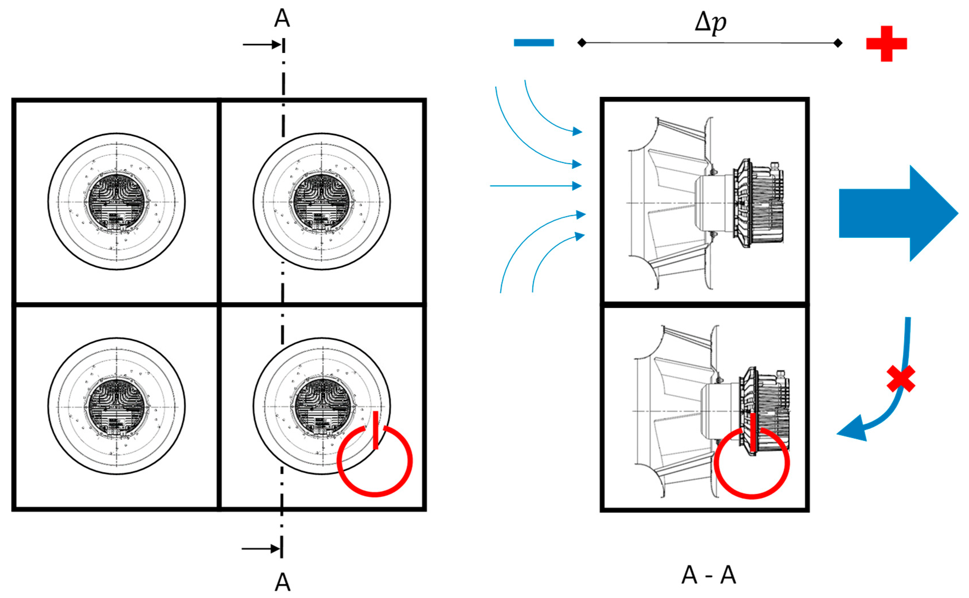
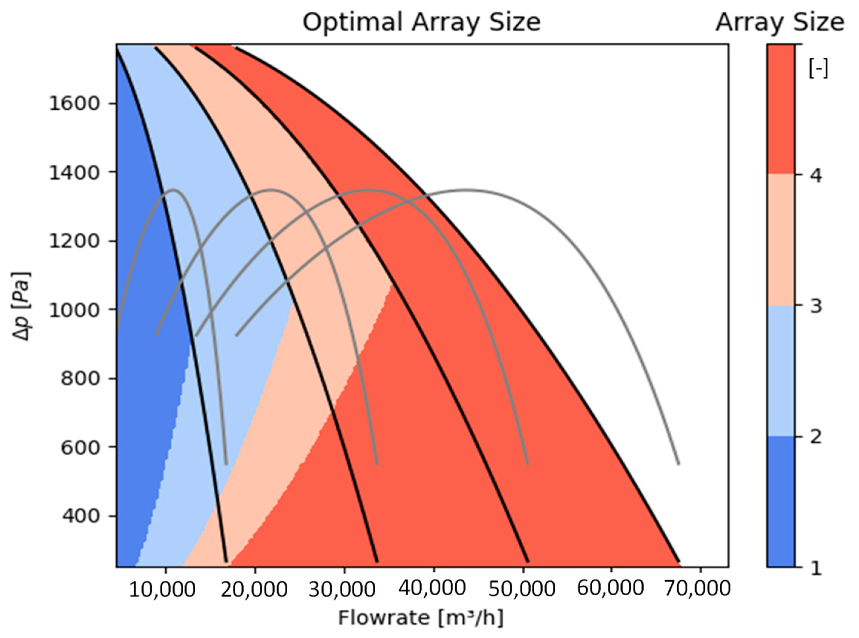
2.2. Variable Array Size with Identical Fans

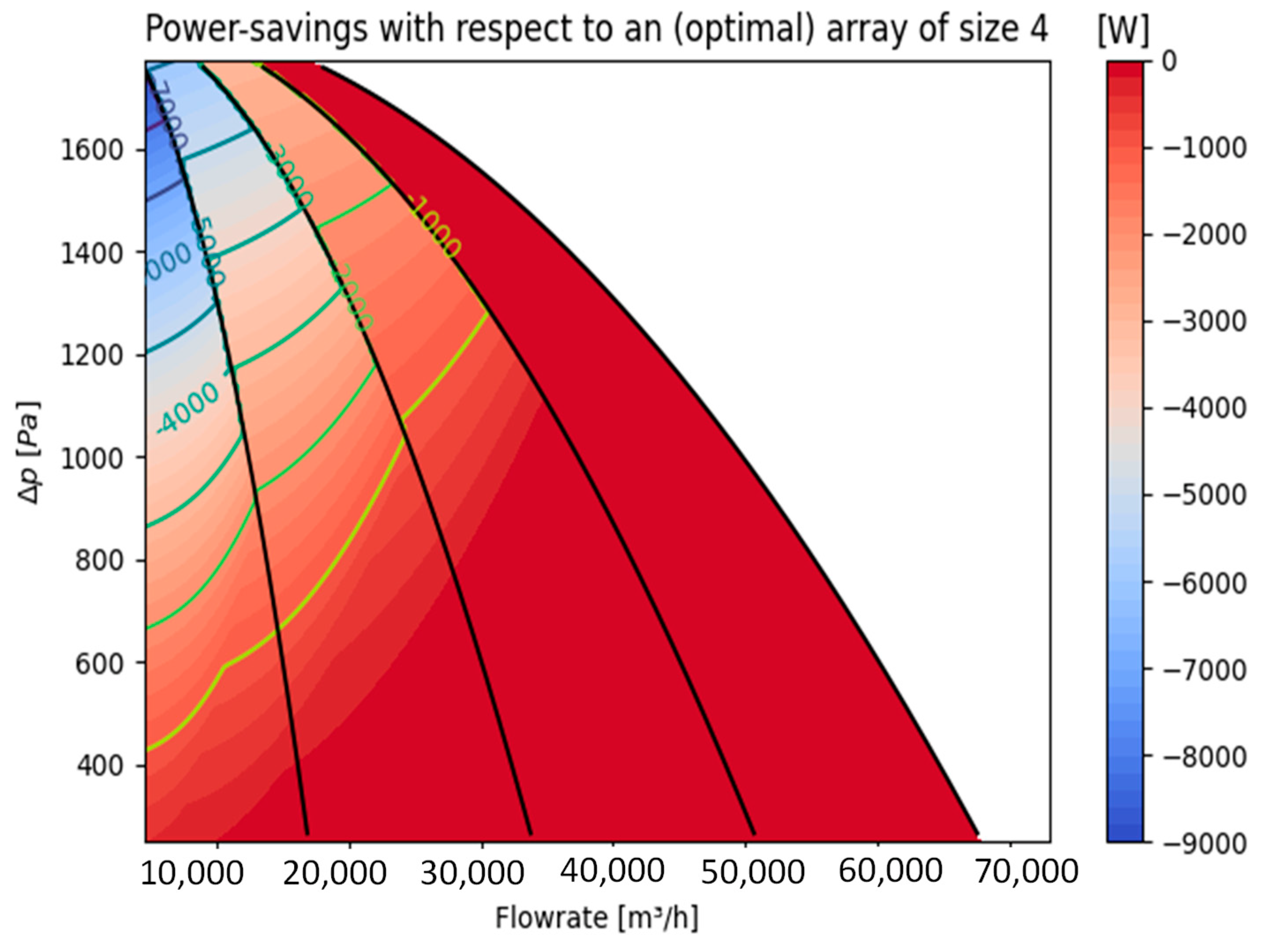
So far, we assumed that all fans of an array with size $k_{max}$ are actively in operation. Now, we investigate possible benefits of selectively turning off one or more fans in such an array. With this modification, the optimization problem becomes a mixed-integer nonlinear programming problem (MINLP).

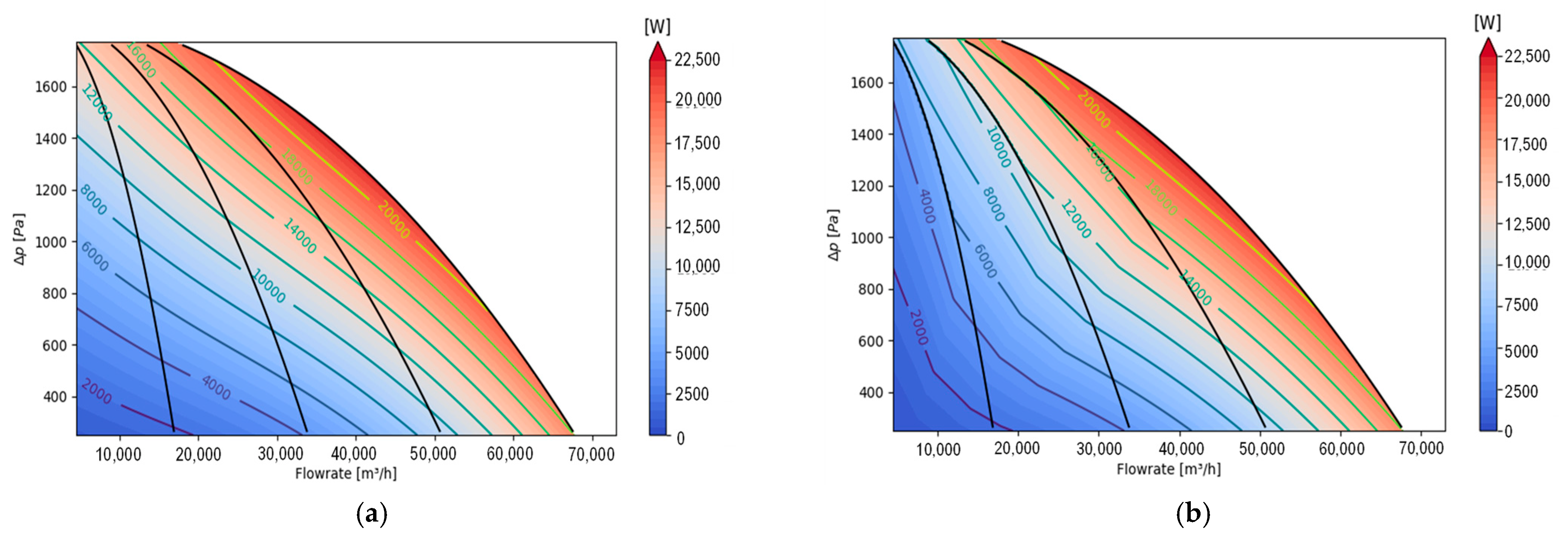
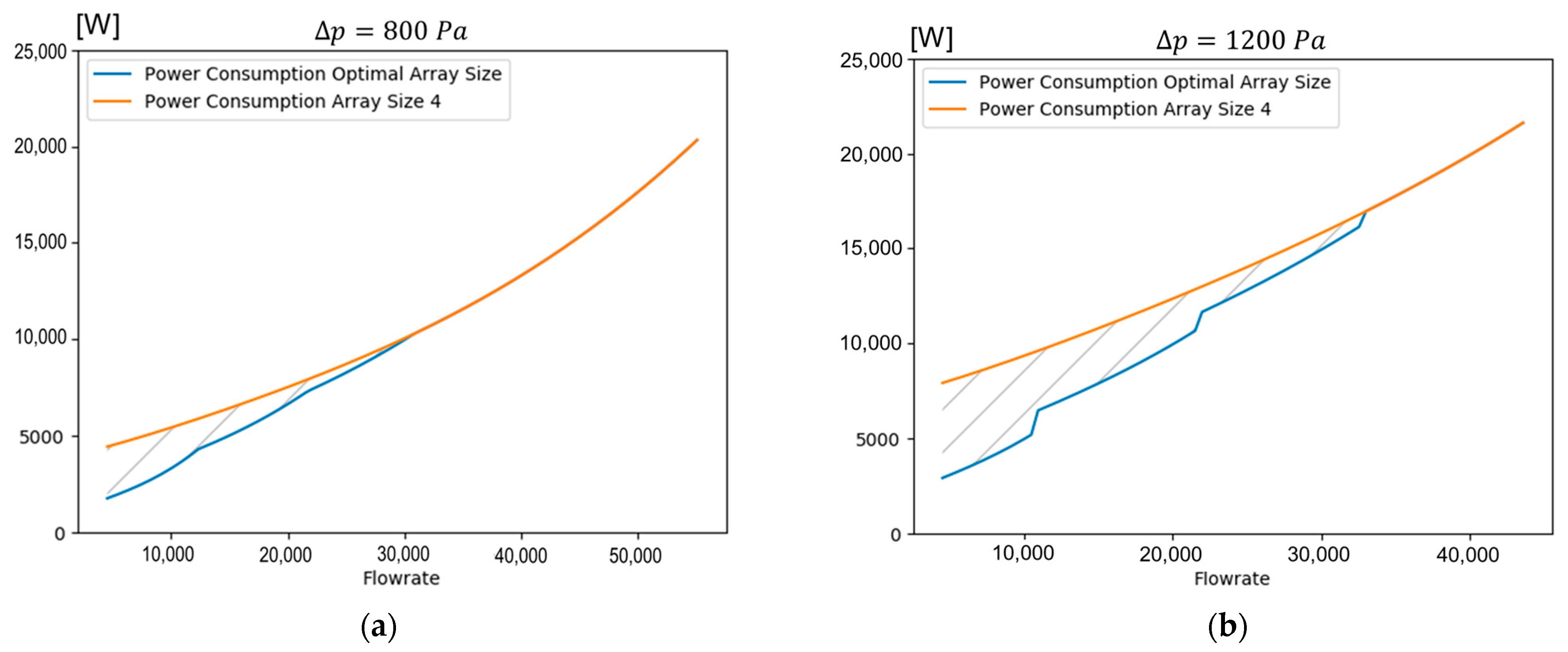
We solve this by applying our method to different array sizes $k=1,2,\dots ,k_{max}$. That means, instead of solving the MINLP directly, we resort to solving a series of NLPs and choose the best configuration in a postprocessing step. In the case of $1\le k\le k_{max}$, we turn off $k_{max}-k$ fans in the array. As stated above, we assume that there is no backflow for turned off fans.

This approach yields the optimal fan speeds along with the corresponding overall power consumption for each of the different arrays sizes. Picking the array size with minimum power consumption yields the optimal array size, i.e., the number of fans to turn off while operating the active fans using their optimal fan speeds.

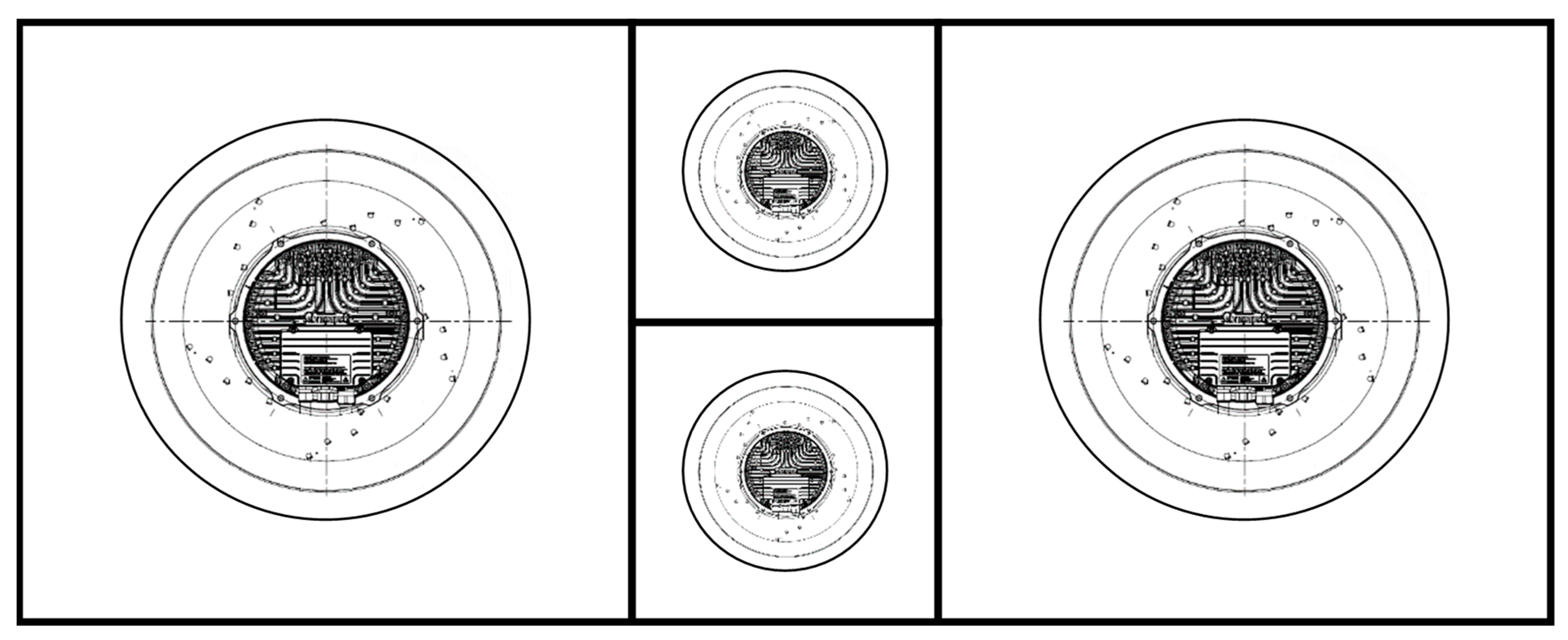
2.3. Variable Array Size with Different Fan Sizes and/or Fan Types

The fans in a parallel setting do not need to be from the same type or size. A possible scenario for an array with different fans is shown in Figure 3:

Our approach is able to account for arrangements where we mix, for example, different sizes of centrifugal fans with different sizes of axial fans. In order to describe this more formally, the fans can vary in their size (D_i) as well as their non-dimensional characteristics described with the coefficients $a_{\psi ,i}, b_{\psi ,i},c_{\psi ,i}, a_{\eta ,i}, b_{\eta ,i}, c_{\eta ,i}, d_{\eta ,i},$ and $e_{\eta ,i}$ in Equations (4), (5), and (8).

In contrast to the approach used for varying array sizes with identical fans, we now have to distinguish between different settings of the array when one or more fans are turned off. This is a problem of unordered sampling without replacement. When shutting down $k_{max}-k$ fans, there are $\frac{k_{max}!}{k!·\left(k_{max}-k\right)!}$ unique possible combinations for the operation of the fan array of size $k<k_{max}$.

For a given operating point, we need to vary the array size and additionally calculate all possible combinations of active fans. This approach yields ${{\displaystyle \sum }}_{k=1}^{k_{max}}\frac{k_{max}!}{k!·\left(k_{max}-k\right)!}$ optimal fan speed combinations, power consumptions, and fan combinations, respectively. The minimum of these power consumptions determines the optimal array size $k_{opt}$ and corresponding $k_{opt}$ fan speeds, as well as the corresponding fan combinations. With this approach, we can assign every operating point in the map with Δ$p_{min}\le \mathsf{\Delta }p\le \mathsf{\Delta }{p}_{max}$ and $Q_{min}\le Q\le Q_{max}$ a $k_{opt}$-tuple of optimal fan speeds and the corresponding optimal combination of active fans, which maximizes the system efficiency, where $k_{max }-k_{opt}$ fans are turned off, respectively.

3. Real World Example

For the sake of illustration of our method and without loss of generality, we consider a 2 × 2 fan array consisting of four identical centrifugal fans as depicted in Figure 4:

In order to make the findings more tangible, we omit a non-dimensional presentation and use dimensional values of ebmpapst’s R3G500 centrifugal fan. Applying our method to this 2 × 2 array yields the result in Figure 5 for the operating map of the array where the color bar indicates the number of active fans in the array:

3.1. Discussion of the Operating Map

At very low volume flow rates and pressure levels, it is most efficient to shut down three fans and operate the array with a single fan. With increasing volume flow rate, it becomes advantageous to operate with two fans instead. However, if there is also an increase in pressure demand, it might again be more beneficial to operate in single-fan mode with an adapted fan speed. However, this can only be realized up to the maximum performance of a single fan. Therefore, if the pressure demand further increases, it is mandatory to switch to two-fan mode because a single fan cannot deliver the prescribed volume flow rate anymore, since it already operates at its maximum fan speed. Depending on the operating point this pattern is generalized to higher numbers of active fans.

Additionally, as can be intuitively expected, there is no potential of shutting down any fans in the overload area of the fan array, i.e., in operating points where the full volume flow rate of the array is needed.

3.2. Comparison of an Optimally Controlled Array with on/off Operation to an Optimally Controlled Array without on/off:

The traditional way of improving the efficiency of such an array with identical fans is to synchronously manage the fan speed, as opposed to no control at all (i.e., operation with a fixed fan speed). The optimal way to do this is to apply our method to the full $k_{max}$ sized array, where we compute the fan speeds that minimize the array power consumption across the whole fan map. This would correspond to a classical speed control.

The left plot in Figure 6 shows the solution for the optimally controlled fan array of size 4, where the total number of fans is always active. The color bar, along with some isolines, indicates the total power consumption.

For comparison, there is the solution for the optimally controlled array with optimal array size (this means the number of active fans is variable) on the right-hand side of Figure 6.

In order to highlight the benefits of the new approach, we now have a look at the difference between the two methods of control. Thus, we subtract the values of power consumption of the classical speed control (all fans active) from the power consumption of the variable array approach. We do this for each operating point of the operating map.

Figure 7 shows that, in a moderate area of the operating map, it is already possible to save 1 kW of power consumption, as indicated by the yellow isoline when applying the described new method (with on/off).

Overall, it can be stated that the power consumption savings increase with decreasing volume flow rate and/or increasing pressure demand. The savings are highest in areas with high pressure and low volume flow rate.

This was expected since we can shut down fans in this area of the operating map. Again, there is no saving potential for the power consumption when the operating point can only be met with the full sized array. In this case, the solution of the optimally controlled size 4 array is reproduced.

Another way to investigate the benefits of our on/off approach is to have a look at varying volume flow rates at constant pressure levels. For this purpose, we select two different pressure levels, namely 800 Pa and 1200 Pa as depicted in Figure 8:

Due to the reasons already mentioned, we cannot shutdown any fans in areas with a high volume flow rate. For Δp = 800 Pa, the saving potential kicks in at about 50% of the maximal volume flow rate for this pressure level and increases towards low volume flow rates while gradually reducing the active fan array size.

For the pressure level of 1200 Pa, the saving potential is even more prominent. The onset of the saving potential is already at about 75% of the possible volume flow rate for this pressure level with significantly higher savings for low volume flow rates.

3.3. Design of Fan Arrays

So far, only preexisting arrays were considered. Our method can also be used for the optimal design of new fan arrays.

To this end, we use the approach described above for variably sized arrays. For a given operating point, we consider the diameter of each fan as an additional free variable. Usually, we consider a discrete set of j diameters. By sweeping through the diameter set and subsequent application of our method, we can compute the parameter set, which yields the maximum system efficiency. In a more sophisticated approach, we can also consider the type of fans given by the coefficients $a_{\psi ,i}, b_{\psi ,i},c_{\psi ,i}, a_{\eta ,i}, b_{\eta ,i}, c_{\eta ,i}, d_{\eta ,i},$ and $e_{\eta ,i}$ as additional free variables.

However, it should be noted that the problem size increases exponentially with the number of possible fans to test. This can pose a limit for the exhaustive search used above. A corresponding study will be conducted on how to solve this problem using a reformulation of the equation system (3).

4. Conclusions and Outlook

This work described an innovative method to control fan arrays with the goal of maximizing power savings using optimal fan speeds and the option to selectively shut down one or more fans in the array. This new approach is applicable to arbitrarily shaped fan arrays and a real world example of a 2 × 2 array of ebmpapst’s R3G500 centrifugal fans was examined. It was shown that significant energy savings are possible in areas with moderate to low volume flow rate and/or high pressure level.

This method can also be used to determine an optimal design of fan arrays. Here, the diameter and coefficients that describe the fan characteristics are additional free variables. An in-depth study will be conducted for alternative approaches to the exhaustive search presented for sufficiently small number of possible fans. This is part of future work.

In this work, the target was the minimization of power consumption (optimality condition). We can also allow different target functionals by replacing the aerodynamic power in the system of equations Equation (3) with, e.g., acoustic power. This would enable an operator of fan arrays to control the fan array for minimal sound emission. Alternatively, a multiobjective tradeoff between two or more target functionals is also conceivable. This is also part of future work.

We hope our method is able to make a valuable contribution to the operation and design of fan arrays with the ultimate goal for saving precious energy resources.

References

1. Czwielong, F.; Soldat, J.; Becker, S. On the interactions of the induced flow field of heat exchangers with axial fans. Exp. Therm. Fluid Sci. 2022, 139, 110697. [Google Scholar] [CrossRef]
2. Groß, T.F.; Pöttgen, P.F.; Pelz, P.F. Analytical Approach for the Optimal Operation of Pumps in Booster Systems. J. Water Resour. Plan. Manag. 2017, 143, 04017029. [Google Scholar] [CrossRef]
3. Kallesøe, C.; Aarestrup, J.; Rokkjær, K. Energy optimization for booster sets. World Pumps 2011, 2011, 24–30. [Google Scholar] [CrossRef]
4. Dai, Y.; Jiang, Z.; Chen, P. Decentralized Optimal Control of Variable Speed Parallel-connected Pumps. In Proceedings of the BS2015, the 14th International Conference of the International Building Performance Simulation Association, Hyderabad, India, 7–9 December 2015; pp. 1103–1109. [Google Scholar]
5. Dodge, Y. Lagrange Multiplier. In The Concise Encyclopedia of Statistics; Springer: New York, NY, USA, 2008. [Google Scholar] [CrossRef]
6. Gülich, J.F. Centrifugal Pumps; Springer: New York, NY, USA, 2008. [Google Scholar]
7. Vieira, T.S.; Siqueira, J.R.; Bueno, A.D.; Morales, R.E.M.; Estevam, V. Analytical study of pressure losses and fluid viscosity effects on pump performance during monophase flow inside an ESP stage. J. Pet. Sci. Eng. 2015, 127, 245–258. [Google Scholar] [CrossRef]
Figure 1. Four identical ebmpapst R3G500 centrifugal fans in a 2 × 2 array setup.
Ijtpp 08 00012 g001
Figure 2. Approximation of the non-dimensional fan pressure characteristics: (a) with a second-order polynomial; (b) with a quadratic ansatz.
Ijtpp 08 00012 g002
Figure 3. 2 × 2 fan array with two different sized centrifugal fans.
Ijtpp 08 00012 g003
Figure 4. 2 × 2 fan array with four identical ebmpapst R3G500 centrifugal fans with exemplarily one fan turned off. There is no backflow through the turned off fan.
Ijtpp 08 00012 g004
Figure 5. Fan map with optimal array size. Black solid lines are the pressure curves of a single fan, two fans, three fans, and the whole four-fan array at maximum fan speed, respectively. Grey lines are the corresponding efficiency curves.
Ijtpp 08 00012 g005
Figure 6. Performance map of an array of size 4: (a) with optimal fan speeds; (b) with optimal array size and optimal fan speeds.
Ijtpp 08 00012 g006
Figure 7. Difference between an optimally controlled array of size 4 and an optimally controlled array of optimal size.
Ijtpp 08 00012 g007
Figure 8. Comparison of the power consumption with and without shutdown of fans: (a) for constant pressure of 800 Pa; (b) for constant pressure level of 1200 Pa.
Ijtpp 08 00012 g008
Disclaimer/Publisher’s Note: The statements, opinions and data contained in all publications are solely those of the individual author(s) and contributor(s) and not of MDPI and/or the editor(s). MDPI and/or the editor(s) disclaim responsibility for any injury to people or property resulting from any ideas, methods, instructions or products referred to in the content.