
Experimental Investigation Techniques for Non-Ideal Compressible Fluid Dynamics
Abstract
:1. Introduction
2. Non-Ideal Compressible Fluid Dynamics
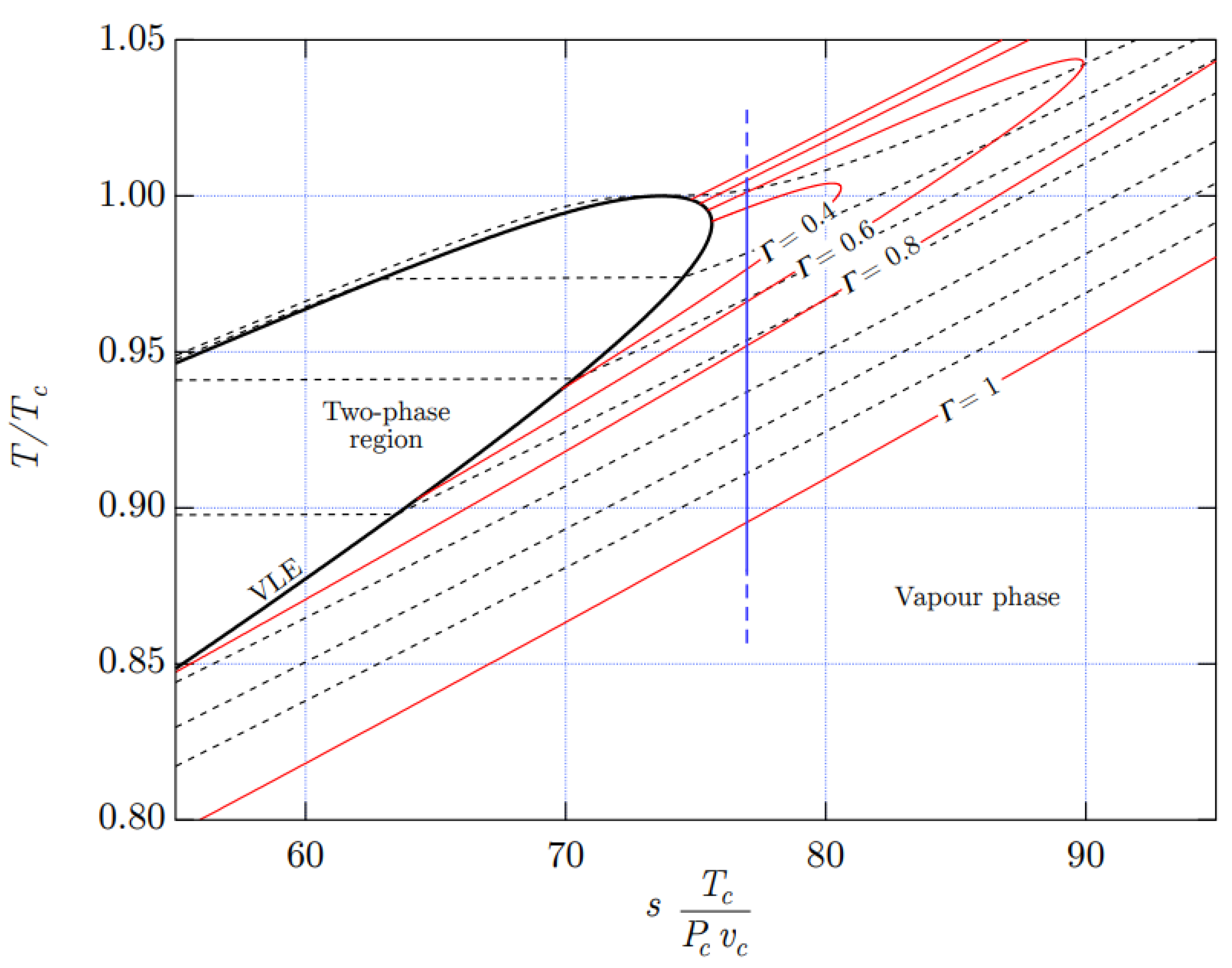
2.1. Thermodynamical Classification of Gas Dynamics

2.2. Classification for Turbomachinery Flows
2.3. Similitude and Experiments with Model Configurations
3. Test Facilities
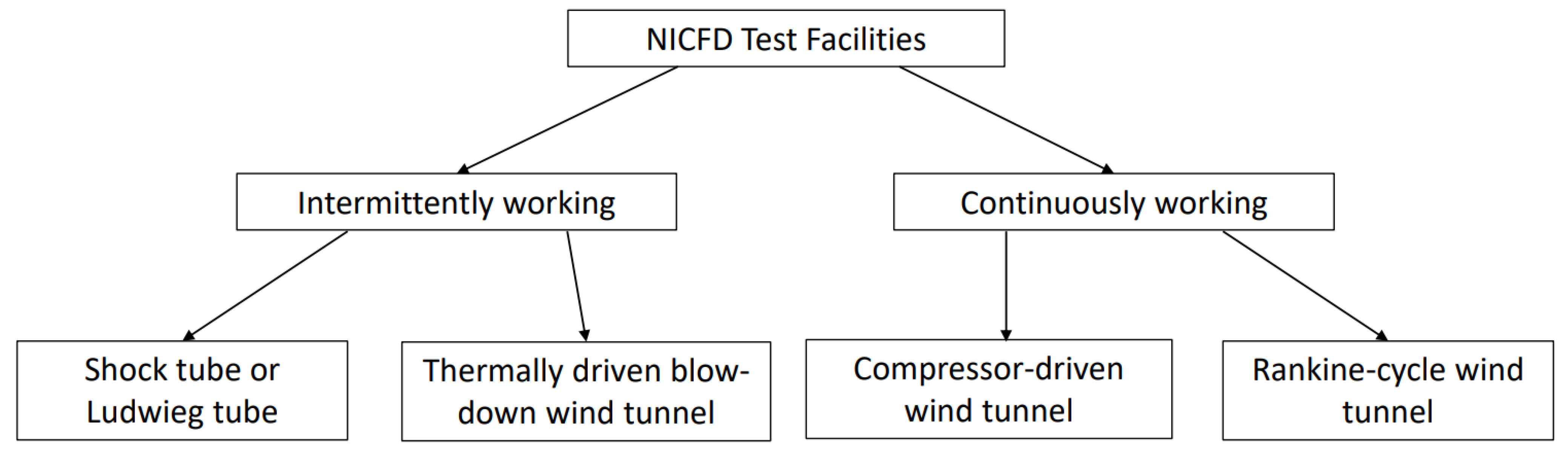
3.1. Classification
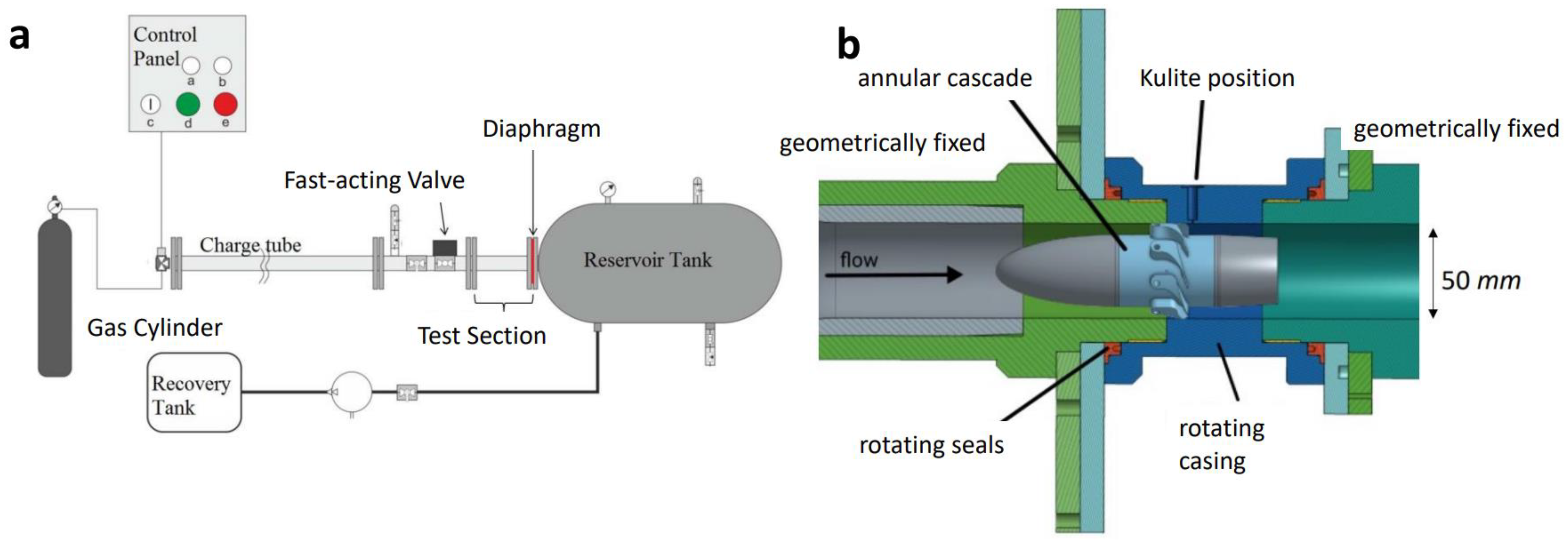
3.2. Shock Tubes or Ludwieg Tubes
3.3. Blow-Down Wind Tunnels
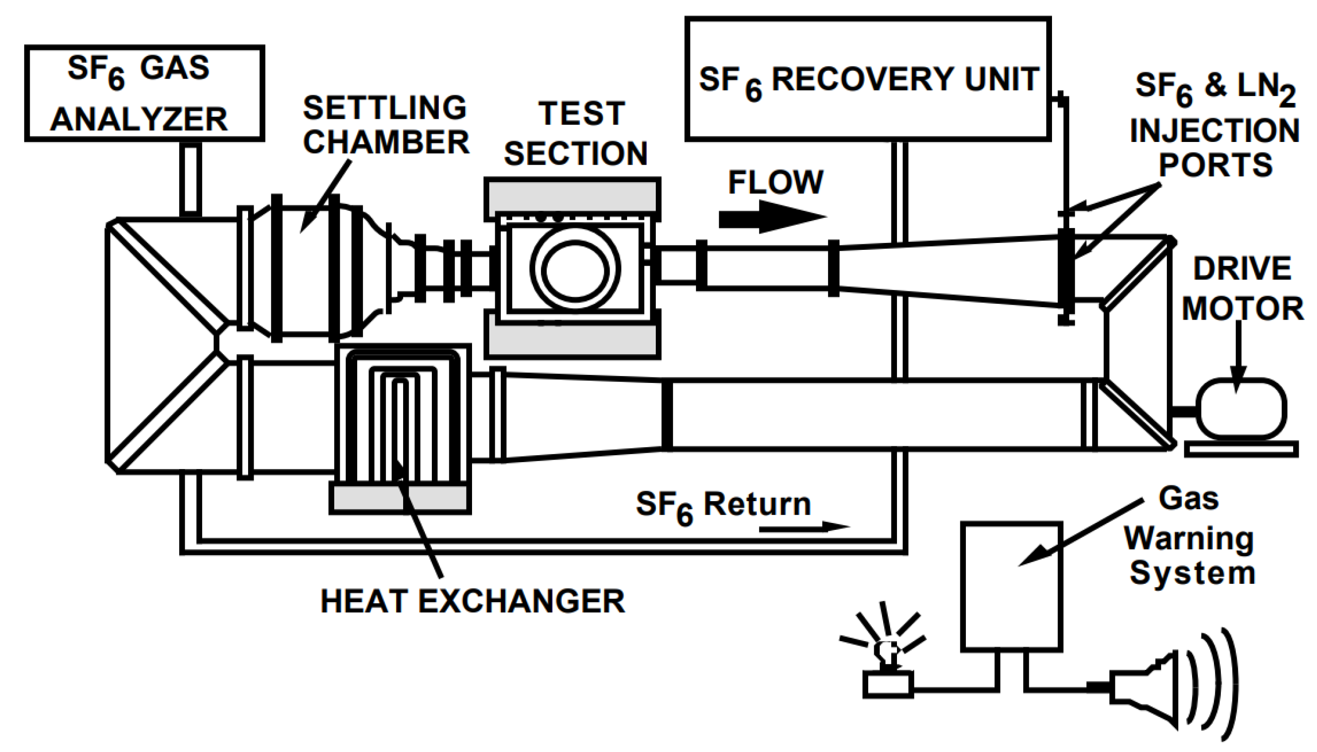
3.4. Compressor-Driven Wind Tunnels
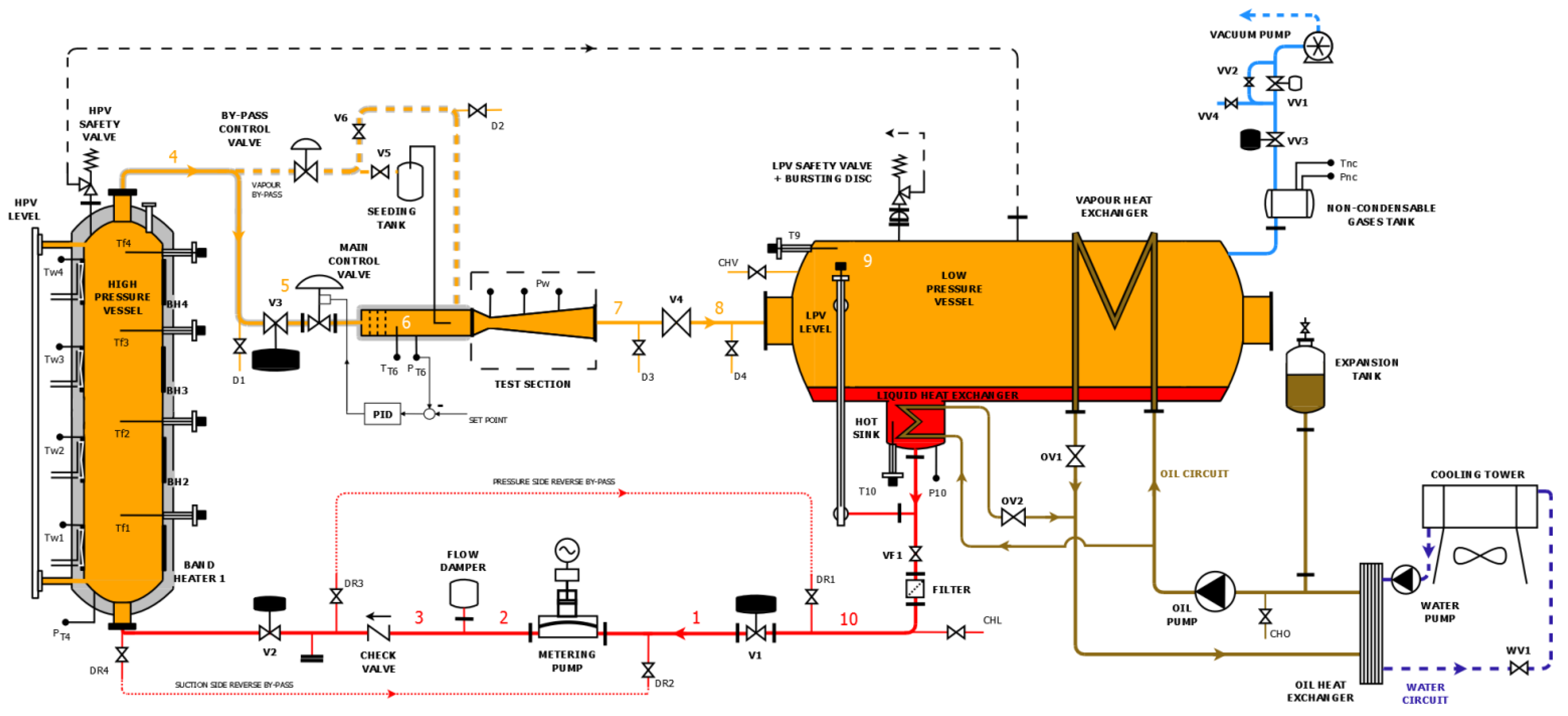
3.5. Rankine Cycle Wind Tunnels
3.6. Current Status of NICFD Test Facilities
4. Pneumatic Measurement Techniques
4.1. Condensation Issues in Organic Vapors
- (i)
- The use of fully heated probes, lines, and pressure measurement devices to avoid any condensation;
- (ii)
- The use of pressure transducers, in combination with lines added by liquid traps and purging devices, to remove condensate or liquid between the probes and the (cooled) measurement devices;
- (iii)
- The use of probes and lines placed in the hot environment of the test rig while considering the condensation as a systematic error.
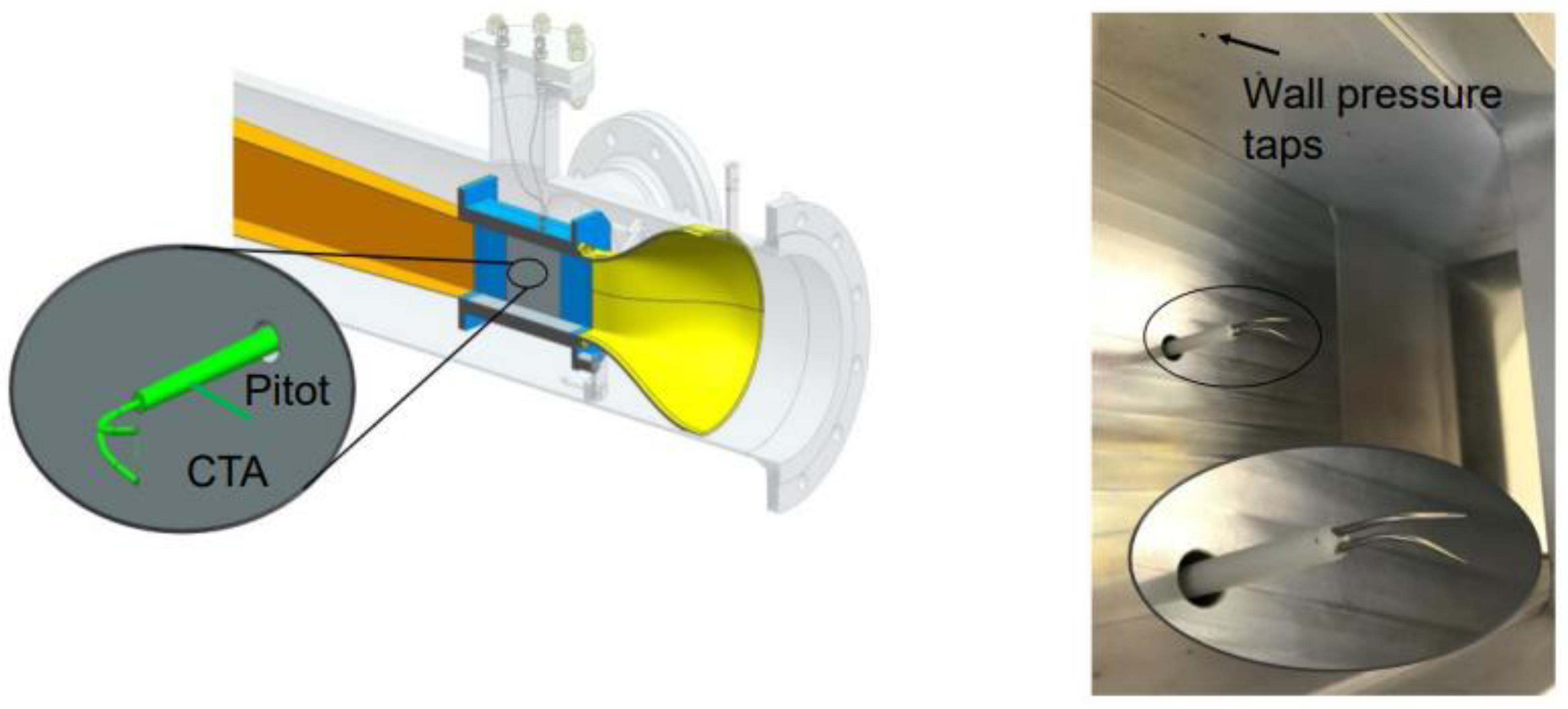
4.2. Pitot and Stagnation Pressure Probes
4.3. Blockage Effects and Probe Interaction
4.4. Pressure Data Reduction for NICFD
5. Optical Measurement Techniques
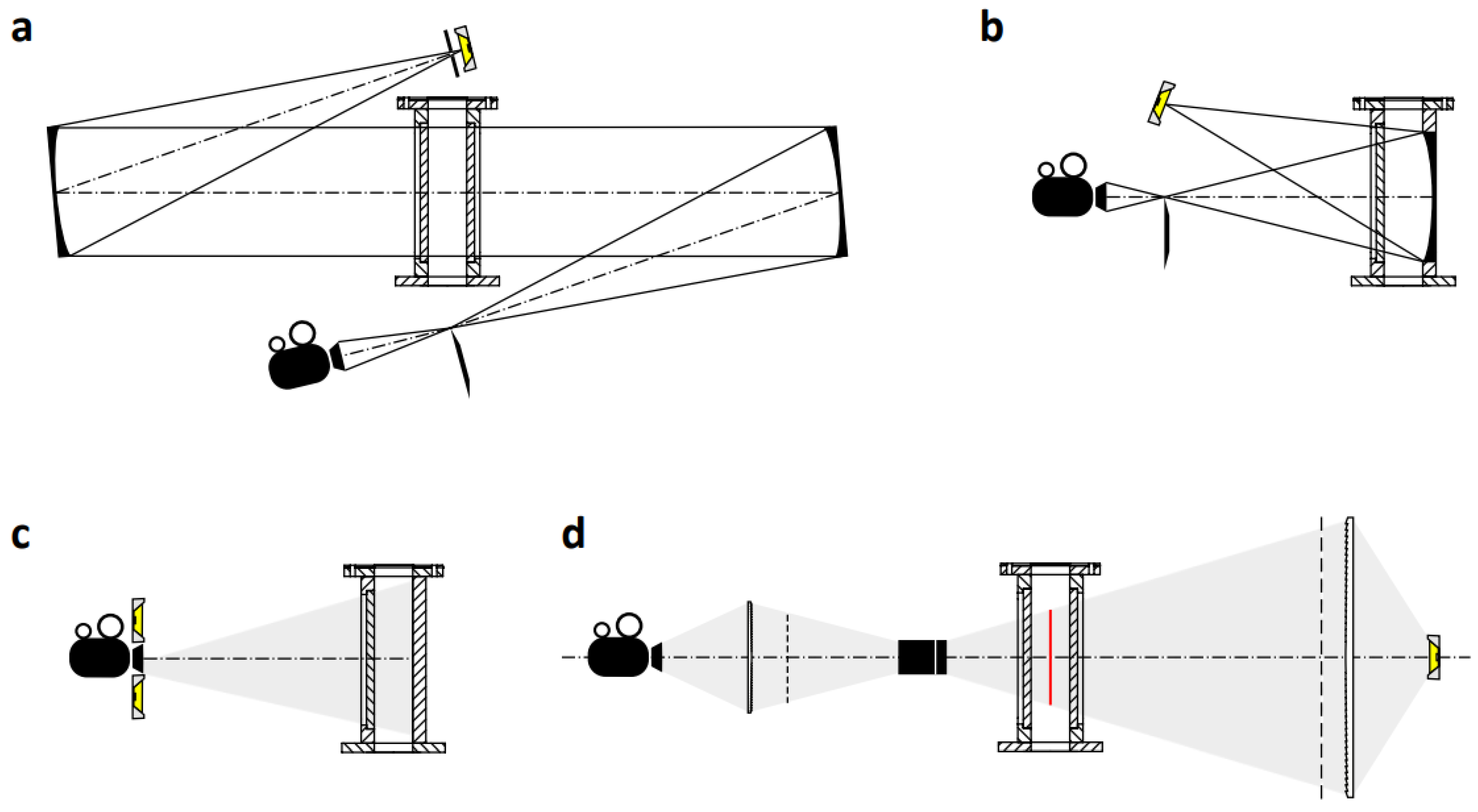
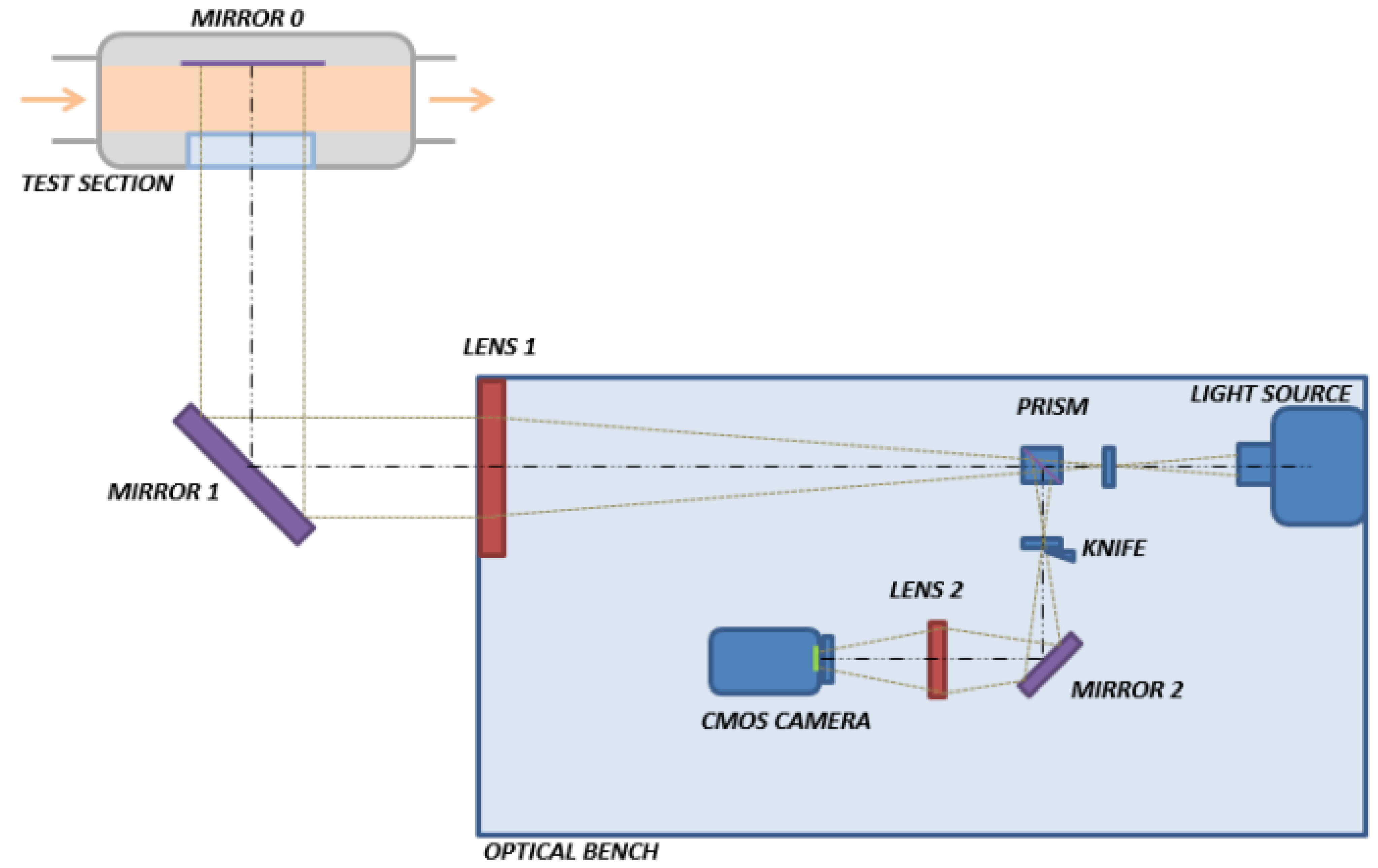
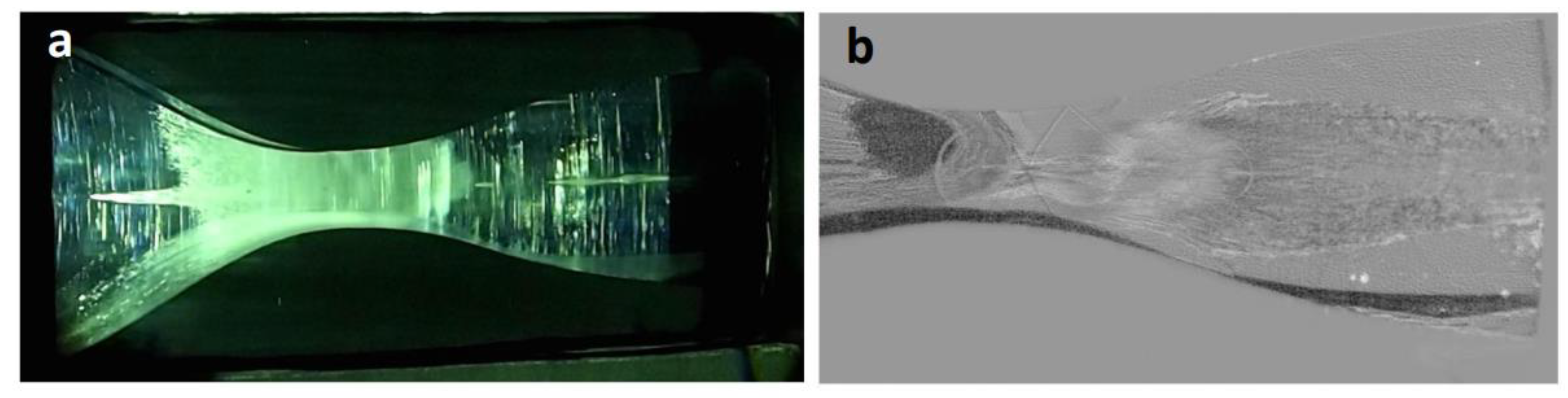
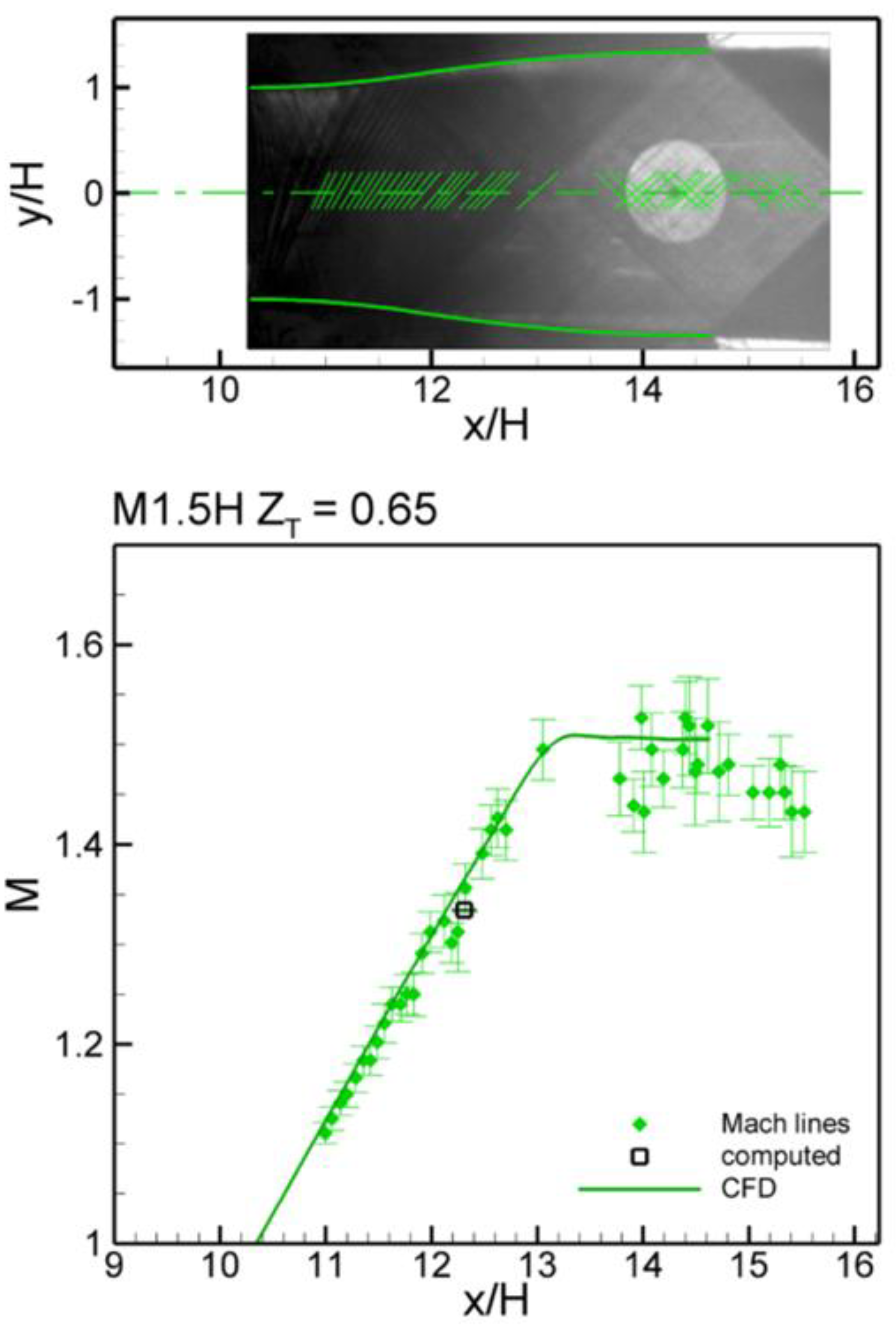
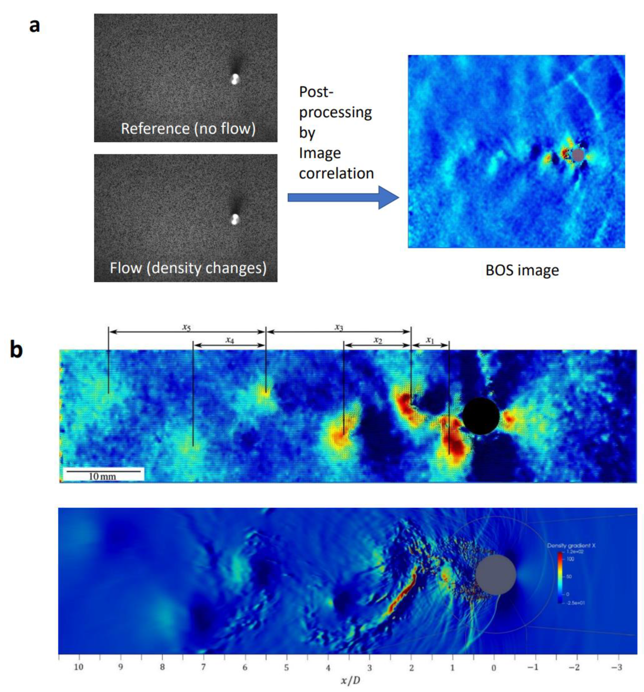
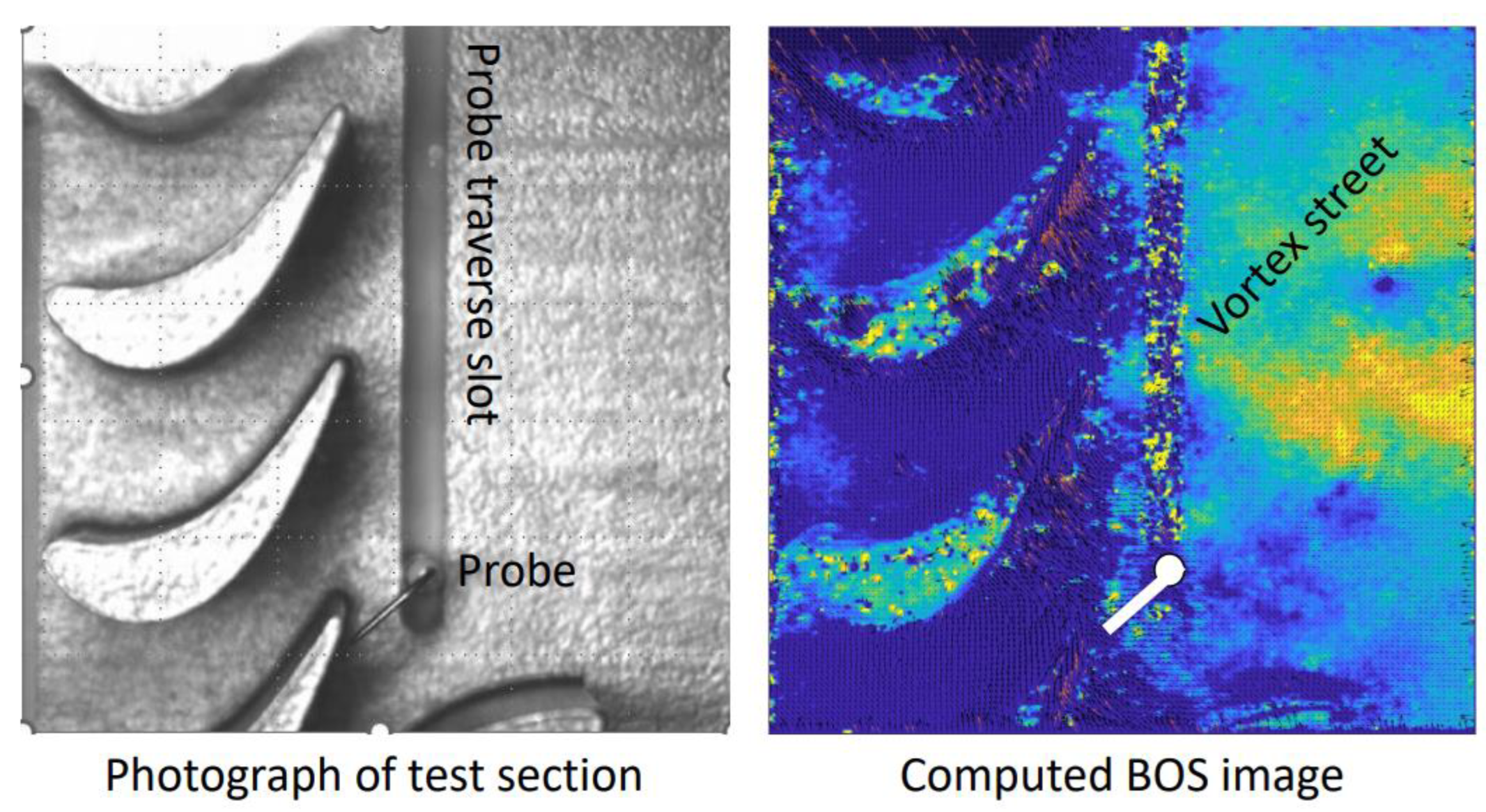
5.1. Schlieren Optical Methods
5.2. Laser Doppler Velocimetry (LDV) Technique
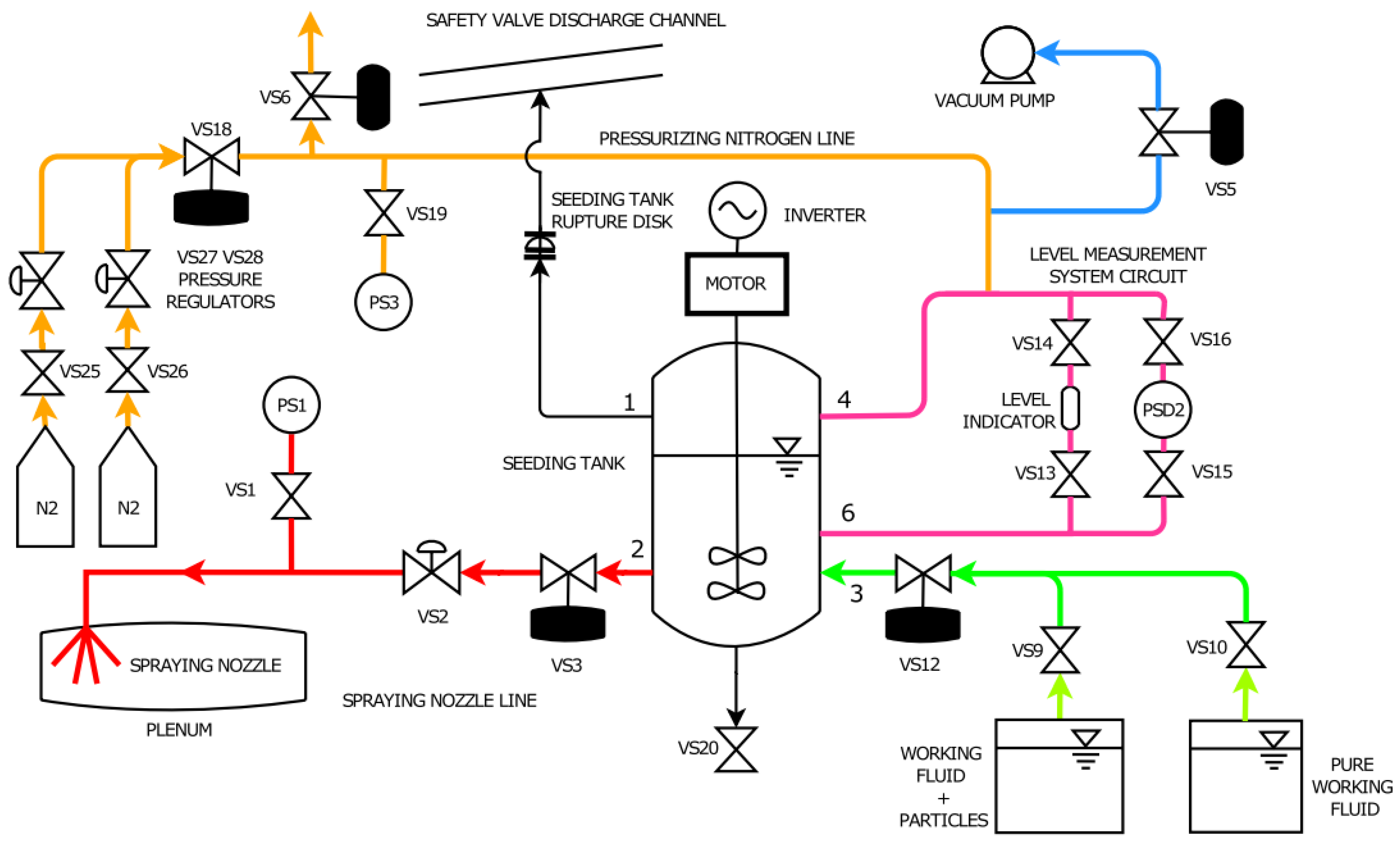
5.3. Particle Image Velocimetry (PIV) Technique
6. Hot-Wire Anemometry
6.1. Calibration and Behavior of Sensitivity Coefficients
6.2. Application and Operational Issues
7. Concluding Remarks
Funding
Institutional Review Board Statement
Informed Consent Statement
Data Availability Statement
Acknowledgments
Conflicts of Interest
Nomenclature
| A | heat transfer correlation coefficient, V2 |
| a | speed of sound, m/s |
| B | heat transfer correlation coefficient |
| c | velocity, m/s |
| cp | isobaric specific heat, J/(kg K) |
| cv | isochoric specific heat, J/(kg K) |
| E | electrical voltage, V |
| f | function, - |
| f | body force, m/s2 |
| h | specific enthalpy, J/kg |
| l | length, m |
| Ma | Mach number, - |
| p | pressure, Pa |
| Pr | Prandtl number, - |
| R | specific gas constant, J/(kg K) |
| Re | Reynolds number, - |
| S | sensitivity coefficient, - |
| S | stress tensor, Pa/m |
| s | specific entropy, J/(kg K) |
| St | Strouhal number, - |
| T | temperature, K |
| t | time, s |
| U | velocity, m/s |
| v | specific volume, m3/kg |
| w | velocity vector, m/s |
| Z | compressibility factor, - |
| Greek symbols | |
| α | angle, ° |
| Γ | fundamental derivative, - |
| γ | isentropic exponent, - |
| ρ | density, kg/m3 |
| λ | thermal conductivity, W/(m K) |
| μ | dynamic viscosity, Pa s |
| η | Kolmogorov length scale, m |
| η | efficiency, - |
| Φ | viscous dissipation, Pa2 |
| ϕ | flow coefficient, - |
| Subscripts | |
| c | critical point |
| o | total or stagnation condition |
| 1 | inflow or upstream of Pitot probe |
| 2 | exit or downstream of Pitot probe shock |
| Superscript | |
| ‘ | fluctuating part |
References
- Colonna, P.; Casati, E.; Trapp, C.; Mathijssen, T.; Larjola, J.; Turunen-Saaresti, T.; Uusitalo, A. Organic Rankine cycle power systems: From the concept to current technology, applications, and an outlook to the future. ASME J. Eng. Gas Turb. Power 2015, 137, 100801. [Google Scholar] [CrossRef] [Green Version]
- Macchi, E.; Astolfi, M. (Eds.) Organic Rankine Cycle (ORC) Power Systems: Technologies and Applications; Woodhead Publishing: Cambridge, UK, 2016. [Google Scholar]
- White, M.T.; Bianchi, G.; Chai, L.; Tassou, S.A.; Sayma, A.I. Review of supercritical CO2 technologies and systems for power generation. Appl. Therm. Eng. 2021, 185, 116447. [Google Scholar] [CrossRef]
- Kluwick, A. Nonlinear Waves in Real Fluids; Springer: Wien, Austria, 1991. [Google Scholar]
- Kluwick, A. Handbook of shockwaves. In Theory of Shock Waves: Rarefaction Shocks; Academic Press: Cambridge, MA, USA, 2001; Volume 1, pp. 339–411. [Google Scholar]
- Kluwick, A. Shock discontinuities: From classical to non-classical shocks. Acta Mech. 2018, 229, 515–533. [Google Scholar] [CrossRef] [Green Version]
- Reynolds, W.C.; Colonna, P. Thermodynamics: Fundamentals and Engineering Applications; Cambridge University Press: Cambridge, UK, 2018. [Google Scholar]
- Guardone, A.; Colonna, P.; Wheeler, A. (Eds.) 1st international seminar on non-ideal compressible fluid dynamics for propulsion and power. J. Physics Conf. Ser. 2017, 821, 011001. [Google Scholar] [CrossRef] [Green Version]
- Duhem, P. On the propagation of shock waves in fluids. Z. Phys. Chem. 1909, 69, 169–186. [Google Scholar] [CrossRef]
- Becker, R. Stoßwelle und Detonation. Z. Für Phys. 1922, 8, 321–362. [Google Scholar] [CrossRef]
- Bethe, H.A. The Theory of Shock Waves for an Arbitrary Equation of State; Report No. 545; Office of Scientific Research and Development: Washington, DC, USA, 1942. [Google Scholar]
- Zel’dovich, Y.B. On the possibility of rarefaction shock waves. Zh. Eksp. Teor. Fiz. 1946, 4, 363–364. [Google Scholar]
- Thompson, P.A. A Fundamental Derivative in Gas Dynamics. Phys. Fluids 1971, 14, 1843–1849. [Google Scholar] [CrossRef]
- Anderson, W.K. Numerical Study on Using Sulfur Hexafluoride as a Wind Tunnel Test Gas. AIAA J. 1991, 29, 2179–2180. [Google Scholar] [CrossRef]
- Anders, J.B. Heavy Gas Wind Tunnel Research at Langley Research Center. ASME Paper. In Proceedings of the Fluids Engineering Conference, Washington, DC, USA, 20–24 June 1993. sponsored by the Fluids Engineering Division, 93-FE-5. [Google Scholar]
- Anders, J.B.; Anderson, W.K.; Murthy, A.V. The Use of Heavy Gas for Increased Reynolds Numbers in Transonic Wind Tunnels. In Proceedings of the 20th AIAA Advanced Measurement and Ground Testing Technology Conference, Albuquerque, NM, USA, 15–18 June 1998. AIAA-98-2882. [Google Scholar]
- Rist, D. Dynamik Realer Gase; Springer: Berlin, Germany, 1996. [Google Scholar]
- Boncinelli, P.; Rubechini, F.; Arnone, A.; Cecconi, M.; Cortese, C. Real gas effects in turbomachinery flows: A computational fluid dynamics model for fast computations. ASME J. Turbomach. 2004, 126, 268–276. [Google Scholar] [CrossRef]
- Brun, K.; Friedman, P.; Dennis, R. (Eds.) Fundamentals and Application of Supercritical Carbon Dioxide Based Power Cycles; Woodhead Publishing: Sawston/Cambridge, UK, 2017. [Google Scholar]
- Head, A.J. Novel Experiments for the Investigation of Non-Ideal Compressible Fluid Dynamics: The ORCHID and First Results of Optical Measurements. Ph.D. Thesis, TU Delft, Delft, The Netherlands, 2021. [Google Scholar]
- Landau, L.D. On shock waves. J. Phys. USSR 1942, 6, 229–230. [Google Scholar]
- Hayes, W.D. The basic theory of gasdynamic discontinuities. In Fundamentals of Gasdynamics; Princeton University Press: Princeton, NJ, USA, 1958; Volume 2. [Google Scholar]
- Vimercati, D.; Gori, G.; Spinelli, A.; Guardone, A. Non-Ideal Effects on the Typical Trailing Edge Shock Pattern of Orc Turbine Blades. Energy Procedia 2017, 129, 1109–1116. [Google Scholar] [CrossRef] [Green Version]
- Colonna, P.; Nannan, N.R.; Guardone, A.; van der Stelt, T.P. On the computation of the fundamental derivative of gas dynamics using equation of states. Fluid Phase Equilibria 2009, 286, 43–54. [Google Scholar] [CrossRef]
- Morren, S.H. Transonic Aerodynamics of Dense Gases; NASA TM-103722; Lewis Research Center: Cleveland, OH, USA, 1991. [Google Scholar]
- Lemmon, E.W.; Huber, M.L.; McLinden, M.O. NIST Reference Database 23: Reference Fluid Thermodynamic and Transport Properties–REFPROP, Version 9.1; Standard Reference Data Program: Gaithersburg, MD, USA, 2013. [Google Scholar]
- Traupel, W. Zur Dynamik realer Gase. Forsch. Ing. 1952, 18, 3–9. [Google Scholar] [CrossRef]
- Traupel, W. Thermische Turbomaschinen—Erster Band, 2nd ed.; Springer: Berlin, Germany, 1966; Chapter 1. [Google Scholar]
- Kouremenos, D.A.; Antonopoulos, K.A. Isentropic Exponents of Real Gases and Application for the Air at Temperatures from 150 K to 450 K. Acta Mech. 1986, 65, 81–99. [Google Scholar] [CrossRef]
- aus der Wiesche, S.; Reinker, F. Dimensional analysis and performance laws for organic vapor flow turbomachinery. Energy 2022, 257, 124635. [Google Scholar] [CrossRef]
- Taylor, E.S. Dimensional Analysis for Engineers; Clarendon: Oxford, UK, 1974. [Google Scholar]
- Dejc, M.E.; Trojanovskij, B.M. Untersuchung und Berechnung Axialer Turbinenstufen; VEB Verlag Technik: Berlin, Germany, 1973. [Google Scholar]
- Turunen-Saaresti, T.; Uusitalo, A.; Honkatukia, J. Design and testing of high temperature micro-ORC test stand using Siloxane as working fluid. In Journal of Physics: Conference Series; IOP Publishing: Bristol, UK, 2017; Volume 821, p. 012024. [Google Scholar]
- Seume, J.R.; Peters, M.; Kunte, H. Design and test of a 10kW ORC supersonic turbine generator. In Journal of Physics: Conference Series; IOP Publishing: Bristol, UK, 2017; Volume 821, p. 012023. [Google Scholar]
- Park, B.S.; Usman, M.; Imran, M.; Pesyridis, A. Review of Organic Rankine Cycle experimental data trends. Energy Convers. Manag. 2018, 173, 679–691. [Google Scholar] [CrossRef]
- Spinelli, A.; Guardone, A.; De Servi, C.; Colonna, P.; Reinker, F.; aus der Wiesche, S.; Robertson, M.; Martinez-Botas, R.F. Experimental facilities for non-ideal compressible vapour flows. ERCOFTAC Bull. 2020, 124, 59–66. [Google Scholar]
- Bradley, J. Shock Waves in Chemistry and Physics; Chapman and Hall: London, UK, 1962. [Google Scholar]
- Gaydon, A.G.; Hurle, I.R. The Shock Tube in High Temperature Chemical Physics; Chapman and Hall: London, UK, 1963. [Google Scholar]
- Soloukhin, R.I. Shock Waves and Detonations in Gases; Mono Books: Baltimore, MD, USA, 1966. [Google Scholar]
- Baumgärtner, D.; Otter, J.J.; Wheeler, A.P. The Effect of Isentropic Exponent on Transonic Turbine Performance. ASME J. Turbomach. 2020, 142, 081007. [Google Scholar] [CrossRef]
- Dura Galiana, F.J.; Wheeler, A.P.; Ong, J. A Study of trailing-edge losses in organic Rankine cycle turbines. In Proceedings of the ASME Turbo Expo 2015: Turbine Technical Conference and Exposition, Montreal, QC, Canada, 15–19 June 2015. GT2015-42920, V02AT38A020, 12p. [Google Scholar]
- Fergason, S.H.; Guardone, A.; Argrow, B.M. Construction and Validation of a Dense Gas Shock Tube. J. Thermophys. Heat Transf. 2003, 17, 326–333. [Google Scholar] [CrossRef]
- Colonna, P.; Guardone, A.; Nannan, N.R.; Zamfirescu, C. Design of the dense gas flexible asymmetric shock tube. ASME J. Fluids Eng. 2008, 130, 034501. [Google Scholar] [CrossRef]
- Mathijssen, T.; Gallo, M.; Casati, E.; Nannan, N.R.; Zamfirescu, C.; Guardone, A.; Colonna, P. The Flexible Asymmetric Shock Tube (FAST): A Ludwieg tube facility for wave propagation measurements in high-temperature vapours of organic fluids. Exp. Fluids 2015, 56, 195. [Google Scholar] [CrossRef] [Green Version]
- Chandrasekaran, N.B.; Michelis, T.; Mercier, B.; Colonna, P. Preliminary experiments in high temperature vapours of organic fluids in the Asymmetric Shock Tube for Experiments on Rarefaction Waves (ASTER). In Proceedings of the 4th International Seminar on Non-Ideal Compressible Fluid Dynamics (NICFD2022), City University, London, UK, 3–4 November 2022. [Google Scholar]
- Dettleff, G.; Thompson, P.A.; Meier, E.A.; Speckmann, H. An experimental study of liquefaction shock waves. J. Fluid Mech. 1979, 95, 279–304. [Google Scholar] [CrossRef]
- Dettleff, G.; Thompson, P.A.; Meier, E.A. Initial experimental results for liquefaction shock waves in organic fluids. Arch. Mech. 1976, 28, 827–836. [Google Scholar]
- Duff, K. Non-Equilibrium Condensation of Carbon Dioxide in Supersonic Nozzles. Ph.D. Thesis, M.I.T., Cambridge, MA, USA, 1966. [Google Scholar]
- Lettieri, C.; Yang, D.; Spakoszky, Z. An investigation of condensation effects in supercritical carbon dioxide compressors. ASME J. Eng. Gas Turbine Power 2015, 137, 082602. [Google Scholar] [CrossRef] [Green Version]
- Spinelli, A.; Dossena, V.; Gaetani, P.; Osnaghi, C.; Colombo, D. Design of a Test Rig for Organic Vapours. In Proceedings of the ASME Turbo Expo 2010, Glasgow, UK, 14–18 June 2010. [Google Scholar]
- Spinelli, A.; Dossena, V.; Gaetani, P.P.; Casella, F. Design, Simulation, and Construction of a Test Rig for Organic Vapors. ASME J. Eng. Gas Turb. Power 2013, 135, 10. [Google Scholar] [CrossRef]
- Spinelli, A.; Guardone, A.; Cozzi, F.; Cammi, G.; Cheli, R.; Zocca, M.; Gaetani, P.; Dossena, V. Experimental Observation of Non-ideal Nozzle Flow of Siloxane Vapor MDM. In Proceedings of the 3rd International Seminar on ORC Power Systems, Brussels, Belgium, 12–14 October 2015. [Google Scholar]
- Spinelli, A.; Cozzi, F.; Cammi, G.; Zocca, M.; Gaetani, P.; Dossena, V.; Guardone, A. Preliminary characterization of an expanding flow of siloxane vapor MDM. In Journal of Physics: Conference Series; IOP Publishing: Bristol, UK, 2017; Volume 821, p. 012022. [Google Scholar]
- Spinelli, A.; Cammi, G.; Conti, C.C.; Gallarini, S.; Zocca, M.; Cozzi, F.; Gaetani, P.; Dossena, V.; Guardone, A. Experimental observation and thermodynamic modeling of non-ideal expanding flows of siloxane MDM vapor for ORC applications. Energy 2019, 168, 285–294. [Google Scholar] [CrossRef]
- Robertson, M.C.; Newton, P.J.; Chen, T.; Martinez-Botas, R.F. Development and commissioning of a blowdown facility for dense gas vapours. In Proceedings of the ASME Turbo Expo 2019, Phoenix, AZ, USA, 17–21 June 2019. GT2019-91609. [Google Scholar]
- Robertson, M.C.; Newton, P.J.; Chen, T.; Costall, A.; Martinez-Botas, R.F. Experimental and numerical study of supersonic non-ideal flows for organic Rankine cycle applications. ASME J. Eng. Gas Turbines Power 2020, 142, 081007. [Google Scholar] [CrossRef]
- Dixon, S.L.; Hall, C.A. Fluid Mechanics and Thermodynamics of Turbomachinery, 6th ed.; Butterworth-Heinemann: Burlington, MA, USA, 2010. [Google Scholar]
- Hirsch, C. (Ed.) Advanced Methods for Cascade Testing; NATO, AGARDograph 328; Specialised Printing Services Limited: Loughton, UK, 1993; ISBN 92-835-0717-7. [Google Scholar]
- Sieverding, C.H. Aerodynamic development of axial turbomachinery blading. In Thermodynamics and Fluid Mechanics of Turbomachinery; Ücer, A.S., Stow, P., Hirsch, C., Eds.; NATO ASI Series: Dordrecht, The Netherlands, 1985; Volume 1. [Google Scholar]
- Reinker, F.; Hasselmann, K.; aus der Wiesche, S.; Kenig, E.Y. Thermodynamics and fluid mechanics of a closed blade cascade wind tunnel for organic vapors. ASME J. Eng. Gas Turbine Power 2015, 138, 052601. [Google Scholar] [CrossRef]
- Reinker, F.; Kenig, E.Y.; Passmann, M.; aus der Wiesche, S. Closed loop organic wind tunnel (CLOWT): Design, components and control system. In Proceedings of the ORC2017—4th International Seminar on ORC Power Systems, Milan, Italy, 13–15 September 2017; pp. 200–207. [Google Scholar]
- Reinker, F.; Kenig, E.Y.; aus der Wiesche, S. CLOWT: A multifunctional test facility for the investigation of organic vapor flows. In Proceedings of the ASME 2018 5th Joint US-European Fluids Engineering Summer Conference, Montreal, QC, Canada, 15–20 June 2018. [Google Scholar]
- Reinker, F.; Kenig, E.Y.; aus der Wiesche, S. Closed loop organic vapor wind tunnel (CLOWT: Commissioning and operational experience. In Proceedings of the ORC2019—5th International Seminar on ORC Power Systems, Athens, Greece, 9–11 September 2019. [Google Scholar]
- Hake, L.; Reinker, F.; Wagner, R.; aus der Wiesche, S.; Schatz, M. The Profile Loss of Additive Manufactured Blades for Organic Rankine Cycle Turbines. Int. J. Turbomach. Propuls. Power 2022, 7, 11. [Google Scholar] [CrossRef]
- White, M.T.; Sayma, A.I. Design of a closed-loop optical access supersonic test facility for organic vapors. In Proceedings of the ASME Turbo Expo 2018, Oslo, Norway, June 11–15 2018. GT2018-75301. [Google Scholar]
- Bier, K.; Ehrler, F.; Hartz, U.; Kissau, G. Zur Berechnung von Düsenströmungen stark realer Gase. Forsch. Lng. Wes. 1977, 43, 175–184. [Google Scholar] [CrossRef]
- Head, A.; De Servi, C.; Casati, E.; Pini, M.; Colonna, P. Preliminary design of the ORCHID: A facility for studying non-ideal compressible fluid dynamics and testing ORC expanders. In Proceedings of ASME Turbo Expo 2016, Seoul, South Korea, 13–17 June 2016. GT2016-56103. [Google Scholar]
- Beltrame, F.; Head, A.J.; De Servi, C.; Pini, M.; Schrijer, F.; Colonna, P. First Experiments and Commissioning of the ORCHID Nozzle Test Section. In NICFD 2020: Proceedings of the 3rd International Seminar on Non-Ideal Compressible Fluid Dynamics for Propulsion; Pini, M., Ed.; ERCOFTAC Series; Springer: Berlin/Heidelberg, Germany, 2021; Volume 28, pp. 169–178. [Google Scholar] [CrossRef]
- White, M. Workshop on experimental test facilities. In Proceedings of the 4th International Seminar on Non-Ideal Compressible Fluid Dynamics (NICFD2022), City University, London, UK, 3–4 November 2022. [Google Scholar]
- Bradshaw, P. Experimental Fluid Mechanics; Pergamon Press: Oxford, UK, 1970. [Google Scholar]
- Bradshaw, P. An Introduction to Turbulence and Its Measurement; Pergamon Press: Oxford, UK, 1971. [Google Scholar]
- Eckelmann, H. Einführung in Die Strömungsmeßtechnik; Teubner: Stuttgart, Germany, 1997. [Google Scholar]
- Nitsche, W.; Brunn, A. Strömungsmesstechnik; Springer-VDI: Berlin, Germany, 2006. [Google Scholar]
- Tropea, C.; Yarin, A.L.; Foss, J.F. (Eds.) Springer Handbook of Experimental Fluid Mechanics; Springer: Berlin, Germany, 2007. [Google Scholar]
- Han, J.-C.; Wright, L. Experimental Methods in Heat Transfer and Fluid Mechanics; CRC Press: Boca Raton, FL, USA, 2022. [Google Scholar]
- Liepmann, H.W.; Roshko, A. Elements of Gasdynamics; John Wiley & Sons: New York, NY, USA, 1957. [Google Scholar]
- John, J.E.; Keith, T.G. Gas Dynamics, 3rd ed.; Pearson: Upper Saddle River, NJ, USA, 2006. [Google Scholar]
- Folsom, R.G. Review of Pitot Tubes. Trans. Am. Soc. Mech. Eng. 1956, 78, 1447–1460. [Google Scholar] [CrossRef]
- Moore, M.J.; Sieverding, C.H. Two-Phase Steam Flow in Turbines and Separators: Theory, Instrumentation, Engineering; Hemisphere Publishing: Washington, DC, USA, 1976; Volume 1. [Google Scholar]
- Murthy, S.; Leonard, M.; Ehresman, C. A Stagnation Pressure Probe for Droplet-Laden Air Flow. J. Propuls. 1986, 2, 195–196. [Google Scholar] [CrossRef]
- Harbeck, J.; Geist, S.; Schatz, M. An approach to measure total-head in wakes and near end walls at high fogging conditions. In Proceedings of the ASME Turbo Expo 2021, Virtual, 7–11 June 2021. GT2021-59190. [Google Scholar]
- Conti, C.; Fusetti, A.; Spinelli, A.; Guardone, A. Shock losses and Pitot tube measurements in non-ideal supersonic and subsonic flows of organic vapors. In Proceedings of the 6th International Seminar on ORC Power Systems, Munich, Germany, 11–13 October 2021; p. 81. [Google Scholar]
- Conti, C.; Fusetti, A.; Spinelli, A.; Gaetani, P.; Guardone, A. Pneumatic system for pressure probe measurements in transient flows of non-ideal vapors subject to line condensation. Measurement 2022, 192, 110802. [Google Scholar] [CrossRef]
- Conti, C.; Fusetti, A.; Spinelli, A.; Guardone, A. Shock loss measurements in non-ideal supersonic flows of organic vapors. Exp. Fluids 2022, 63, 117. [Google Scholar] [CrossRef]
- Reinker, F.; Wagner, R.; Passmann, M.; Hake, L.; aus der Wiesche, S. Performance of a rotatable cylinder pitot probe in high subsonic non-ideal gas flows. In NICFD 2020, ERCOFTAC Series 28; Pini, M., de Servi, C., Spinelli, A., di Mare, F., Guardone, A., Eds.; Springer International Publishing: Cham, Switzerland, 2021; pp. 144–152. [Google Scholar] [CrossRef]
- aus der Wiesche, S.; Reinker, F.; Wagner, R.; Hake, L.; Passmann, M. Critical and choking Mach numbers for organic vapor flows through turbine cascades. In Proceedings of the ASME Turbo Expo 2021, Virtual, 7–11 June 2021. GT2021-59013. [Google Scholar]
- Dura Galiana, F.J.; Wheeler, A.P.; Ong, J. A Study of trailing-edge losses in organic Rankine cycle turbines. Proc. ASME J. Turbomach. 2016, 138, 121003. [Google Scholar] [CrossRef]
- Reinker, F.; Wagner, R.; Hake, L.; aus der Wiesche, S. High subsonic flow of an organic vapor past a circular cylinder. Exp. Fluids 2021, 62, 54. [Google Scholar] [CrossRef]
- Manfredi, M.; Persico, G.; Spinelli, A.; Gaetani, P.; Dossena, V. Loss measurement strategy in ORC supersonic blade cascades. In Proceedings of the 4th International Seminar on Non-Ideal Compressible Fluid Dynamics (NICFD2022), City University, London, UK, 3–4 November 2022. [Google Scholar]
- Manfredi, M.; Spinelli, A.; Persico, G.; Gaetani, P.; Dossena, V. Nitrogen experiments on a supersonic linear cascade for ORC applications. In Proceedings of the XXVI Biennial Symposium on Measuring Techniques in Turbomachinery, Pisa, Italy, 28–30 September 2022. [Google Scholar]
- Baumgärtner, D. Real Gas Effects in ORC Turbines. Ph.D. Thesis, University of Cambridge, Cambridge, UK, 2020. [Google Scholar] [CrossRef]
- Wyler, J.S. Probe Blockage Effects in Free Jets and Closed Tunnels. ASME J. Eng. Power 1975, 97, 509–514. [Google Scholar] [CrossRef]
- Truckenmüller, F.; Renner, M.; Stetter, H.; Hosenfeld, H. Transonic probe blockage effects in a calibration wind-tunnel and stator blade passage. In Proceedings of the ASME Turbo Expo 1996, Birmingham, UK, 10–13 June 1996; pp. 1–8. [Google Scholar]
- Langford, R.W.; Keeley, K.R.; Wood, N.B. Investigation of the Transonic Calibration Characteristics of Turbine Static Pressure Probes. In Proceedings of the ASME 1982 International Gas Turbine Conference and Exhibit, London, UK, 18–22 April 1982. ASME-Paper, No. 82-GT-280. [Google Scholar]
- Squire, L.C. Effects of Probe Supports on Measurements in Steam Turbines. In Proceedings of the ASME 1986 International Gas Turbine Conference and Exhibit, Dusseldorf, Germany, 8–12 June 1986. ASME-Paper, No. 86-GT-213. [Google Scholar]
- Ducruet, C. A Method for Correcting Wall Pressure Measurements in Subsonic Compressible Flow. ASME J. Fluids Eng. 1991, 113, 256–260. [Google Scholar] [CrossRef]
- Spinelli, A.; Cammi, G.; Gallarini, S.; Zocca, M.; Cozzi, F.; Gaetani, P.; Dossena, V.; Guardone, A. Experimental evidence of non-ideal compressible effects in expanding flow of a high molecular complexity vapor. Exp. Fluids 2018, 59, 126. [Google Scholar] [CrossRef] [Green Version]
- Schollmeier, J.-N.; aus der Wiesche, S. A user-friendly pitot probe data reduction routine for non-ideal gas flow applications. Energy 2022, 261, 125143. [Google Scholar] [CrossRef]
- Passmann, M.; aus der Wiesche, S.; Joos, F. A one-dimensional analytical calculation method for obtaining normal shock losses in supersonic real gas flows. In Journal of Physics: Conference Series; IOP Publishing: Bristol, UK, 2017; Volume 821, p. 012004. [Google Scholar] [CrossRef]
- Span, R.; Wagner, W. Equations of state for technical applications. I. Simultaneously optimized functional forms for nonpolar and polar fuids. Int. J. Thermophys. 2003, 24, 1–39. [Google Scholar] [CrossRef]
- Colonna, P.; Nannan, N.R.; Guardone, A.; Lemmon, E.W. Multiparameter equations of state for selected siloxanes. Fluid Phase Equilibria 2006, 244, 193–211. [Google Scholar] [CrossRef]
- Colonna, P.; Nannan, N.R.; Guardone, A. Multiparameter equations of state for siloxanes[(CH3)3-Si-O1/2]2-[O-Si-(CH3)2]i=1,...,3, and [O-Si-(CH3)2]6. Fluid Phase Equilibria 2008, 263, 115–130. [Google Scholar] [CrossRef]
- Thol, M.; Dubberke, F.H.; Rutkai, G.; Windmann, T.; Köster, A.; Span, R.; Vrabec, J. Fundamental equation of state correlation for hexamethyldisiloxane based on experimental and molecular simulation data. Fluid Phase Equilibria 2016, 418, 133–151. [Google Scholar] [CrossRef]
- Thol, M.; Dubberke, F.H.; Baumhögger, E.; Vrabec, J.; Span, R. Speed of sound measurements and fundamental equations of state for octamethyltrisiloxane and decamethyltetrasiloxane. J. Chem. Eng. Data 2017, 62, 2633–2648. [Google Scholar] [CrossRef]
- Gori, G.; Molesini, P.; Persico, G.; Guardone, A. Non-Ideal Compressible-Fluid Dynamics of Fast-Response Pressure Probes for Unsteady Flow Measurements in Turbomachinery. In Journal of Physics: Conference Series; IOP Publishing: Bristol, UK, 2017; Volume 821, p. 012005. [Google Scholar]
- Cozzi, F.; Spinelli, A.; Gallarini, S.; Guardone, A. Optical Diagnostics for Non-Ideal Compressible Fluid Dynamics. Rcoftac Bull. 2020, 124, 67–72. [Google Scholar]
- Head, A.J.; Novara, M.; Gallo, M.; Schrijer, F.; Colonna, P. Feasibility of Particle Image Velocimetry for Low-Speed Unconventional Vapor Flows. Exp. Therm. Fluid Sci. 2019, 102, 589–594. [Google Scholar] [CrossRef]
- Settles, G.S. Schlieren and Shadowgraph Techniques: Visualizing Phenomena in Transparent Media; Springer: Berlin/Heidelberg, Germany, 2001. [Google Scholar]
- Merzkirch, W. Flow Visualization; Academic Press: Cambridge, MA, USA, 1987. [Google Scholar]
- Conti, C.C.; Spinelli, A.; Cammi, G.; Zocca, M.; Cozzi, F.; Guardone, A. Schlieren visualizations of non-ideal compressible fluid flows. In Proceedings of the 13th International Conference on Heat Transfer, Fluid Mechanics and Thermodynamics (HEFAT 2017); EDAS: Messina, Italy, 2017; pp. 513–518. [Google Scholar]
- Cammi, G. Measurements Techniques for Non-Ideal Compressible Fluid Flows: Applications to Organic Fluids. Ph.D. Thesis, Politecnico di Milano, CREA Lab, Milan, Italy, 2019. [Google Scholar]
- Zocca, M.; Guardone, A.; Cammi, G.; Cozzi, F.; Spinelli, A. Experimental observation of oblique shock waves in steady non-ideal flows. Exp. Fluids 2019, 60, 101. [Google Scholar] [CrossRef] [Green Version]
- Cozzi, F.; Göttlich, E.; Angelucci, L.; Dossena, V.; Guardone, A. Development of a background oriented schlieren technique with telecentric lenses for supersonic flow. In Journal of Physics: Conference Series; IOP Publishing: Bristol, UK, 2017; Volume 778, p. 012006. [Google Scholar]
- Richard, H.; Raffel, M. Principle and applications of the background oriented schlieren (BOS) method. Meas. Sci. Technol. 2001, 12, 1576–1585. [Google Scholar] [CrossRef]
- Klinge, F.; Kirmse, T.; Kompenhans, J. Application of Quantitative Background Oriented Schlieren (BOS): Investigation of a Wing Tip Vortex in a Transonic Wind Tunnel. Proc. PSFVIP4 2003, 4097, 3–5. [Google Scholar]
- Goldhahn, E.; Seume, J. The background oriented schlieren technique: Sensitivity, accuracy, resolution and application to a three-dimensional density field. Exp. Fluids 2007, 43, 241–249. [Google Scholar] [CrossRef]
- Venkatakrishnan, L.; Meier, G.E. Density measurements using the Background Oriented Schlieren technique. Exp. Fluids 2004, 37, 237–247. [Google Scholar] [CrossRef] [Green Version]
- Raffel, M. Background-oriented schlieren (BOS) techniques. Exp. Fluids 2015, 56, 1–17. [Google Scholar] [CrossRef] [Green Version]
- Clem, M.M.; Zaman, K.B.M.Q.; Fagan, A.F.; Glenn, N. Background Oriented Schlieren Applied to Study Shock Spacing in a Screeching Circular Jet. In Proceedings of the 50th AIAA Aerospace Sciences Meeting including the New Horizons Forum and Aerospace Exposition, Nashville, TN, USA, 9–12 January 2012; pp. 1–12. [Google Scholar]
- Kindler, K.; Goldhahn, E.; Leopold, F.; Raffel, M. Recent developments in background oriented Schlieren methods for rotor blade tip vortex measurements. Exp. Fluids 2007, 43, 233–240. [Google Scholar] [CrossRef]
- Sundermeier, S.; Matar, C.; aus der Wiesche, S.; Cinnella, P.; Hake, L.; Gloerfelt, X. Experimental and numerical study of transonic flow of an organic vapor past a circular cylinder. In Proceedings of the 4th International Seminar on Non-Ideal Compressible Fluid Dynamics (NICFD2022), City University, London, UK, 3–4 November 2022. [Google Scholar]
- Passmann, M.; aus der Wiesche, S.; Joos, F. Focusing Schlieren Visualization of Transonic Turbine Tip-Leakage Flows. Int. J. Turbomach. Propuls. Power 2020, 5, 1. [Google Scholar] [CrossRef] [Green Version]
- Schardin, H. Die Schlierenverfahren und ihre Anwendungen. In Ergebnisse der Exakten Naturwissenschaften; Springer: Berlin, Germany, 1942; pp. 303–349. [Google Scholar]
- Weinstein, L. Large-Field High-Brightness Focusing Schlieren System. AIAA J. 1993, 31, 1250–1255. [Google Scholar] [CrossRef]
- Albrecht, H.-E.; Damaschke, N.; Borys, M.; Tropea, C. Laser Doppler and Phase Doppler Measurement Techniques; Springer: Berlin, Germany, 2013. [Google Scholar]
- Gallarini, S.; Cozzi, F.; Spinelli, A.; Guardone, A. Direct velocity measurements in high-temperature non-ideal vapor flows. Exp. Fluids 2021, 62, 199. [Google Scholar] [CrossRef]
- Gallarini, S.; Spinelli, A.; Cozzi, F.; Guardone, A. Design and commissioning of a laser doppler velocimetry seeding system for non-ideal fluid flows. In Proceedings of the 12th International Conference on Heat Transfer, Fluid Mechanics and Thermodynamics HEFAT, Costa de Sol, Spain, 11–13 July 2016. [Google Scholar]
- Westerweel, J.; Elsinga, G.E.; Adrian, R.J. Particle image velocimetery for complex and turbulent flow. Annu. Rev. Fluid Mech. 2013, 45, 409–436. [Google Scholar] [CrossRef]
- Raffel, M.; Willert, C.E.; Wereley, S.T.; Kompenhans, J. Particle Image Velocimetry: A Practical Guide; Springer: Berlin, Germany, 2007. [Google Scholar]
- Ueno, W.; Tsuru, S.; Kinoue, Y.; Shiomo, N.; Setoguchi, T. PIV measurement of carbon dioxide gas-liquid two-phase nozzle flow. In Proceedings of the ASME-JSME-KSME Joints Fluids Engineering Conference, Seoul, Republic of Korea, 26–31 July 2015. AJKFluids2015-20169. [Google Scholar]
- Valori, V. Rayleigh-Benard Convection of A Supercritical Fluid: (PIV) and Heat Transfer Study. Ph.D. Thesis, Delft University of Technology, Delft, The Netherlands, 2017. [Google Scholar]
- Perry, A. Hot-Wire-Anemometry; Clarendon Press: Oxford, UK, 1982. [Google Scholar]
- Fingerson, L.; Freymuth, P. Thermal Anemometers. In Fluid Mechanics Measurements; Goldstein, R., Ed.; Hemisphere: Washington, DC, USA, 1983. [Google Scholar]
- Lomas, C. Fundamentals of Hot Wire Anemometry; Cambridge University Press: Cambridge, UK, 1986. [Google Scholar]
- Bruun, H.H. Hot-Wire Anemometry: Principles and Signal Analysis; Oxford University Press: Oxford, UK, 1995. [Google Scholar]
- Comte-Bellot, G. Hot-Wire Anemometry. Annu. Rev. Fluid Mech. 1976, 8, 209–231. [Google Scholar] [CrossRef]
- Kovasznay, L.S.G. The Hot-Wire Anemometer in Supersonic Flows. J. Aeronaut. Sci. 1950, 17, 565–584. [Google Scholar] [CrossRef]
- Spangenberg, W.G. Heat Loss Characteristics of Hot-Wire Anemometers at Various Densities in Transonic and Supersonic Flow; NACA Tech. Note No. 3381; National Advisory Committee for Aeronautics: Washington, DC, USA, 1955. [Google Scholar]
- Morkovin, M.W. Fluctuations and Hot-Wire Anemometry in Compressible Flows; AGARDograph No. 24; NATO: Paris, France, 1956. [Google Scholar]
- Horstman, C.C.; Rose, W.C. Hot-Wire Anemometry in Transonic Flow. AIAA J. 1977, 15, 395–401. [Google Scholar]
- Rose, W.C.; McDaid, E.P. Turbulence Measurement in Transonic Flow. AIAA J. 1977, 15, 1368–1370. [Google Scholar] [CrossRef]
- Stainback, P.C.; Johnson, C.B.; Basnett, C.B. Preliminary Measurements of Velocity, Density and Total Temperature Fluctuations in Compressible Subsonic Flow. In Proceedings of the AIAA 21st Aerospace Sciences Meeting, Reno, NV, USA, 10–13 January 1983. AIAA-83-0384. [Google Scholar]
- Stainback, P.C. Some Influences of Approximate Values for Velocity, Density and Total Temperature Sensitivities on Hot Wire Anemometer Results. In Proceedings of the AIAA 24th Aerospace Sciences Meeting, Reno, NV, USA, 6–9 January 1986. AIAA-86-0506. [Google Scholar]
- Stainback, P.C.; Nagabushana, K.A. Review: Hot-Wire Anemometry in Transonic and Subsonic Slip Flows. ASME Fluids Eng. 1997, 119, 14–18. [Google Scholar] [CrossRef]
- Motallebi, F. A Review of the Hot-Wire Technique in 2-D Compressible Flows. Prog. Aerospace Sci. 1994, 30, 267–294. [Google Scholar] [CrossRef]
- Johnston, R.; Fleeter, S. Compressible flow hot-wire calibration. Exp. Fluids 1997, 22, 444–446. [Google Scholar] [CrossRef]
- de Souza, F.; Tavoularis, S. Hot-Wire Response in High-Subsonic Flow. In Proceedings of the AIAA 37th Aerospace Sciences Meeting and Exhibit, Reno, NV, USA, 11–14 January 1999. AIAA-99-0310. [Google Scholar]
- Cukurel, B.; Acarer, S.; Arts, T. A novel perspective to high-speed cross-hot-wire calibration methodology. Exp. Fluids 2012, 53, 1073–1085. [Google Scholar] [CrossRef]
- Reinker, F.; aus der Wiesche, S. Application of Hot-Wire Anemometry in the High Subsonic Organic Vapor Flow Regime. In NICFD 2020, ERCOFTAC Series 28; Pini, M., de Servi, C., Spinelli, A., di Mare, F., Guardone, A., Eds.; Springer International Publishing: Cham, Switzerland, 2021; pp. 135–143. [Google Scholar]
- Hake, L.; Sundermeier, S.; Cakievski, L.; Bäumer, J.; aus der Wiesche, S.; Matar, C.; Cinnella, P.; Gloerfelt, X. Hot-Wire Anemometry in High Subsonic Organic Vapor Flows. In Proceedings of the ASME Turbo Expo 2022, Rotterdam, The Netherlands, 13–17 June 2022. GT2022-81686. [Google Scholar]
- Hake, L.; aus der Wiesche, S.; Sundermeier, S.; Bienner, A.; Gloerfelt, X.; Cinnella, P. Grid-generated decaying turbulence in an organic vapor flow. In Proceedings of the 4th International Seminar on Non-Ideal Compressible Fluid Dynamics (NICFD2022), City University, London, UK, 3–4 November 2022. [Google Scholar]
- Jones, G.S. Wind Tunnel Requirements for Hot-Wire Calibration. In Proceedings of the AIAA 18th Aerospace Ground Testing Meeting, Colorado Springs, CO, USA, 20–23 June 1994. AIAA-94-2534. [Google Scholar]
- Yavuzkurt, S. A Guide to Uncertainty Analysis of Hot-Wire Data. ASME J. Fluids Eng. 1984, 106, 181–186. [Google Scholar] [CrossRef]
- Smolyakov, A.V.; Tkachenko, V.M. The Measurement of Turbulent Fluctuations; Springer: Berlin, Germany, 1983. [Google Scholar]
- Wyngaard, J.C. Measurement of small-scale turbulence structure with hot wires. J. Sci. Instrum. 1968, 1, 1105–1108. [Google Scholar] [CrossRef]
- Hake, L.; Sundermeier, S.; aus der Wiesche, S.; Bienner, A.; Gloerfelt, X.; Matar, C.; Cinnella, P. CFD-supported data reduction of hot-wire anemometry signals for compressible organic vapor flows. In Proceedings of the XXVI Biennial Symposium on Measuring Techniques in Turbomachinery, Pisa, Italy, 28–30 September 2022. [Google Scholar]
- Weiss, J.; Chokani, N.; Comte-Bellot, G. Constant-Temperature and Constant-Voltage Anemometer Use in a Mach 2.5 Flow. AIAA J. 2005, 43, 1140–1143. [Google Scholar] [CrossRef]
- Roediger, T.; Jenkins, S.; Knauss, H.; Wolfersdorf, J.; Gaisbauer, U.; Kraemer, E. Time-Resolved Heat Transfer Measurements on the Tip Wall of a Ribbed Channel Using a Novel Heat Flux Sensor—Part I: Sensor and Benchmarks. ASME J. Turbomach. 2008, 130, 011018. [Google Scholar] [CrossRef]
- Sieverding, C.; Manna, M. A Review on Turbine Trailing Edge Flow. Int. J. Turbomach. Propuls. Power 2020, 5, 10. [Google Scholar] [CrossRef]
- Sieverding, C.H.; Heinemann, H. The Influence of Boundary Layer State on Vortex Shedding from Flat Plates and Turbine Cascades. ASME J. Turbomach. 1990, 112, 181–187. [Google Scholar] [CrossRef]


| Γ | Fluid | Sound Speed Variation | Classification of Gas Dynamics |
|---|---|---|---|
| Γ > 1 | Perfect gas | classical | |
| Γ = 1 | classical non-ideal | ||
| Γ < 1 | Dense gas | classical non-ideal | |
| Γ = 0 | non-classical non-ideal | ||
| Γ < 0 | BZT fluids | non-classical non-ideal |
| Z | Fluid | Example | Aerodynamic Testing |
|---|---|---|---|
| Z = 1 | Perfect gas | Air | conventional wind tunnel testing |
| Z = f(s) | Perfect vapor | Steam | mainly conventional (correction schemes applicable) |
| f(s) | Non-ideal gas | Organic vapors | correction schemes might not apply |
| Test Facility | Institution | Type and Operation mode | Measurement Times | Working Fluids | Pressure | Temperature | Mach Number | Minimum Z/Γ | Test Section |
|---|---|---|---|---|---|---|---|---|---|
| TROVA | Milano, IT | Blow-down wind tunnel | 10 up to 100 s | Siloxanes, refrigerants, hydrocarbons | Up to 50 bar | Up to 400 °C | Up to Ma = 3 | Z = 0.3/Γ < 1 | 50 mm × 100 mm |
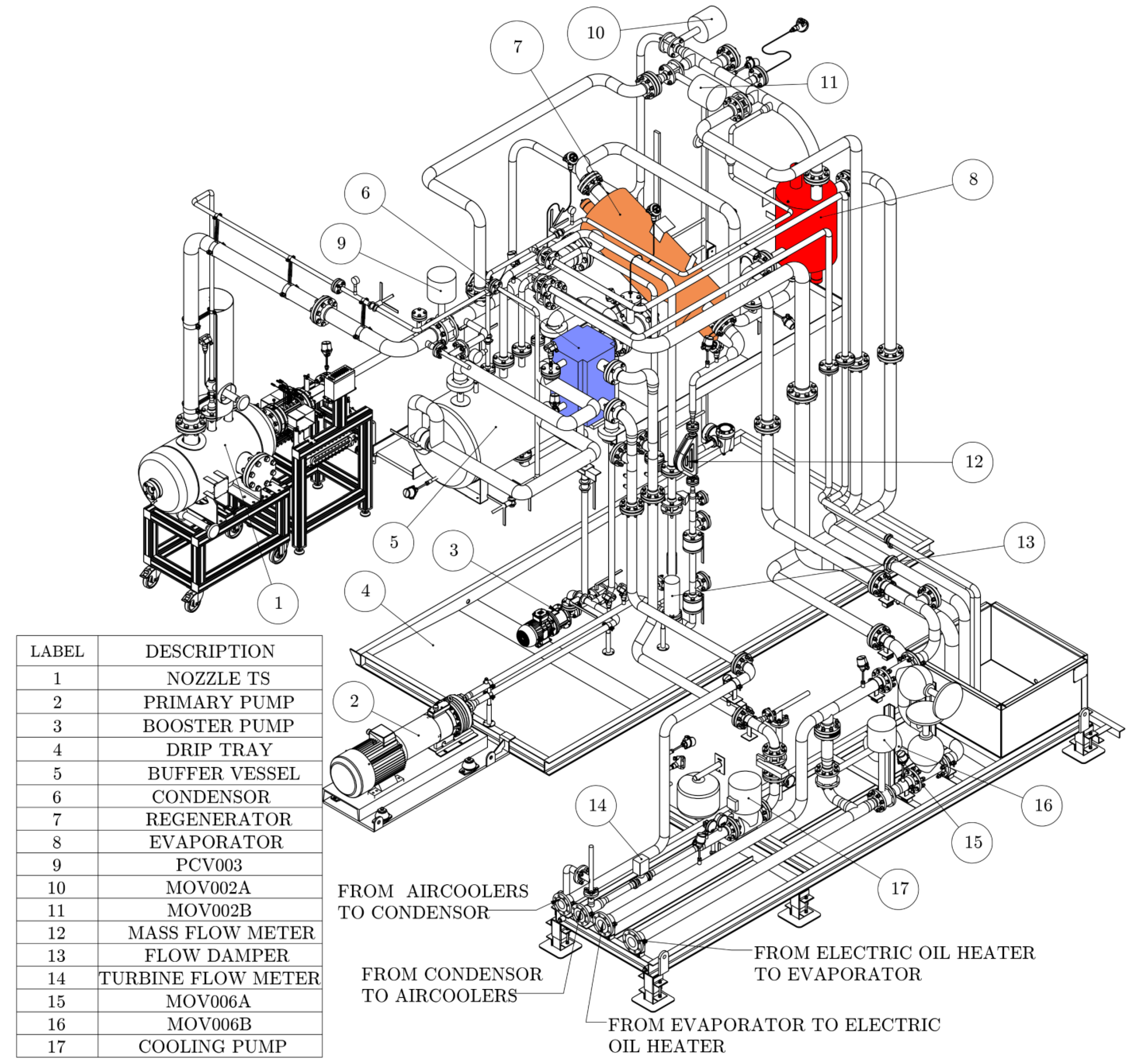
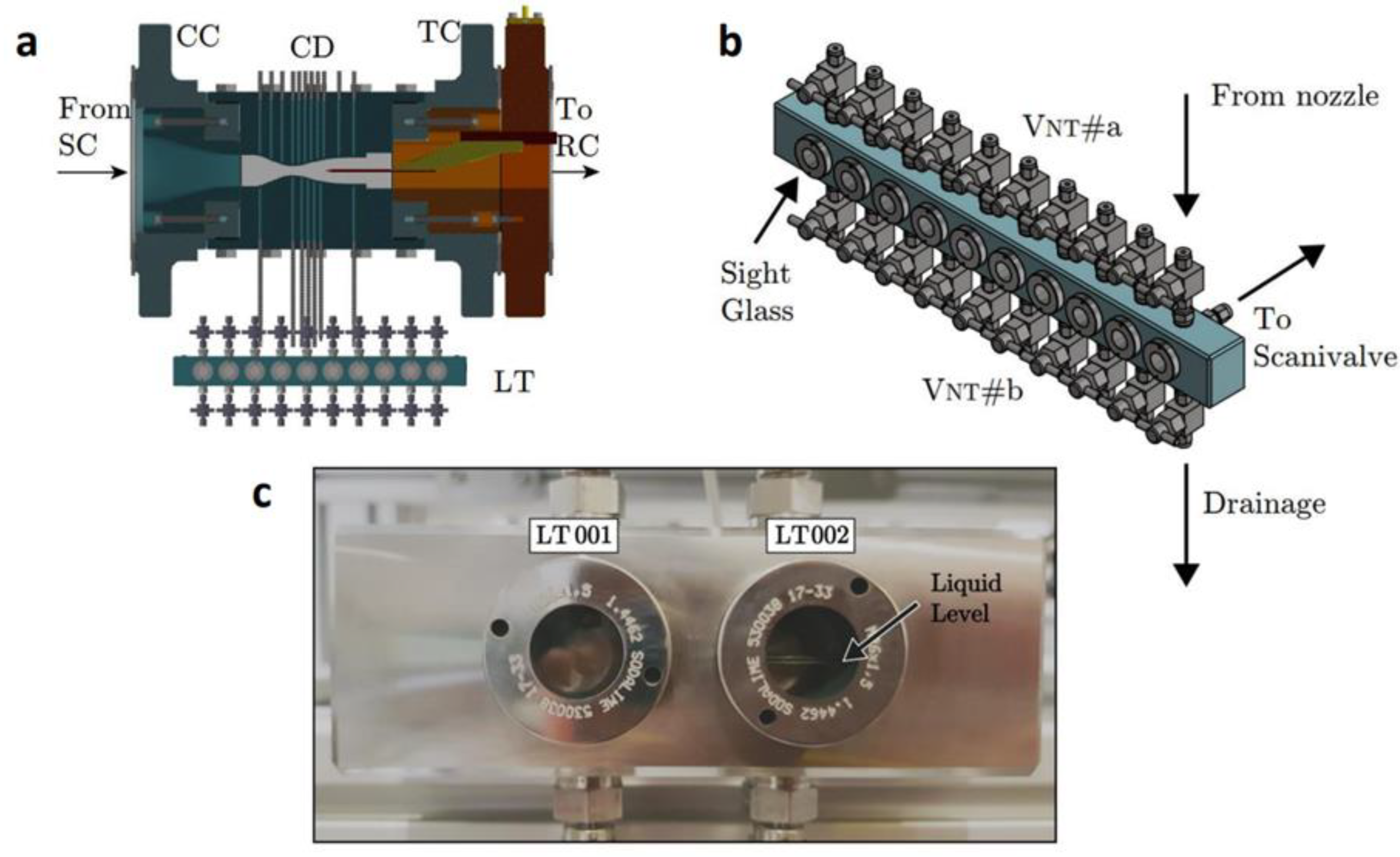
| ORCHID | TU Delft, NL | Rankine wind tunnel (continuously) | Long time | Siloxanes, refrigerants, hydro-carbons | Up to 25 bar | Up to 380 °C | Up to Ma = 3 | Z = 0.3/Γ < 1 | Limited by thermal power (400 kW) |
| CLOWT | FH Münster, DE | Closed wind tunnel (continuously) | Long time | Novec 649, air | Up to 10 bar | Up to 150 °C | Up to Ma = 1.3 | Z = 0.7/Γ = 0.8 | 50 mm × 100 mm or 42 diameter (jet) |
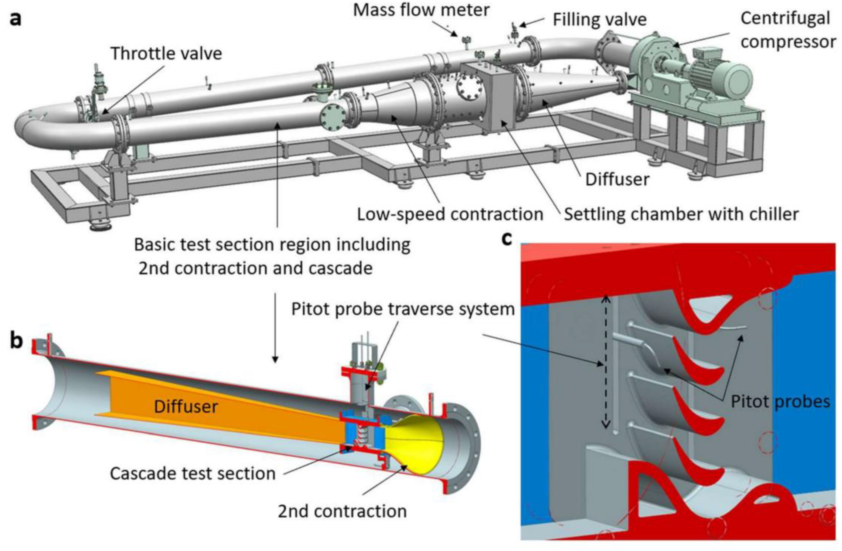
| Cambridge Real-Gas Wind Tunnel | Whittle, UK | Ludwieg tube | 10–100 ms | R134a, SF6, CO2, Air, N2, Argon | Up to 45 bar | 15–150 °C | Up to Ma = 2.5 | Z = 0.6/Γ < 0.9 | 50 mm tube diameter |
| ICLTRANSIENT | Imperial, UK | Blow-down wind tunnel | Short time | Refrigerants | Up to 30 bar | 70 °C (nominal) | Up to Ma = 2.2 | Z = 0.5/Γ = 1.05 | 2 mm throat height |
| Material | Refractive Index | Density | Melting Temperature |
|---|---|---|---|
| TiO2 | 2.6 up to 2.9 | 3900–4200 kg/m3 | 1840 °C |
| Al2O3 | 1.79 | 3960 kg/m3 | 2015 °C |
| SiO2 | 1.45 | 2200 kg/m3 | 1710 °C |
| SiC | 2.6 | 3200 kg/m3 | 2700 °C |
Disclaimer/Publisher’s Note: The statements, opinions and data contained in all publications are solely those of the individual author(s) and contributor(s) and not of MDPI and/or the editor(s). MDPI and/or the editor(s) disclaim responsibility for any injury to people or property resulting from any ideas, methods, instructions or products referred to in the content. |
© 2023 by the author. Licensee MDPI, Basel, Switzerland. This article is an open access article distributed under the terms and conditions of the Creative Commons Attribution (CC BY-NC-ND) license (https://creativecommons.org/licenses/by-nc-nd/4.0/).
Share and Cite
Wiesche, S.a.d. Experimental Investigation Techniques for Non-Ideal Compressible Fluid Dynamics. Int. J. Turbomach. Propuls. Power 2023, 8, 11. https://doi.org/10.3390/ijtpp8020011
Wiesche Sad. Experimental Investigation Techniques for Non-Ideal Compressible Fluid Dynamics. International Journal of Turbomachinery, Propulsion and Power. 2023; 8(2):11. https://doi.org/10.3390/ijtpp8020011
Chicago/Turabian StyleWiesche, Stefan aus der. 2023. "Experimental Investigation Techniques for Non-Ideal Compressible Fluid Dynamics" International Journal of Turbomachinery, Propulsion and Power 8, no. 2: 11. https://doi.org/10.3390/ijtpp8020011