1. Introduction
The evaluation and reduction of the emitted sound is an important part of the development of new fans. Especially in applications that operate close to humans, such as air conditioning or kitchen hoods, quiet fans are requested. In contrast to the measurements of the standalone fan, typically used in the development process, in applications, the acoustics can be significantly influenced by disturbed inflow conditions. As shown by Lucius et al. [
1], even a rectangular box in front of the fan drastically increases the emitted sound, whereas the effect on the aerodynamic properties is only minor.
Evaluations of the aerodynamic properties with numerical simulations using CFD (Computational Fluid Dynamics) are commonly used in the development process of new fans. Due to increased computational resources, CAA (Computational Aeroacoustics) methods have become more important in predicting the emitted sound and identifying sound-generating mechanisms. As shown by Lucius et al. [
1], scale-resolving simulations such as LES (Large Eddy Simulation) are able to correctly calculate the acoustics of fans. However, a high computational effort is needed to resolve upstream structures, which influence the inflow conditions. For axial fans, a typical application is in combination with a heat exchanger unit. This is, for example, the case in heat pumps, where the fan is often installed after the heat exchanger. The shape and geometric details of the heat exchanger lead to a non-uniform turbulent flow field which will interact with the fan blades during operation. This can significantly increase the emitted sound. Due to the complex geometry (thinly stacked fins and cooling rods) and the dimensions of heat exchangers, a very high computational effort (estimated mesh size for resolution of typical heat exchanger: ~1 × 10
10 cells) is needed to resolve all the necessary details. In a product development process, this is currently not economically feasible.
Turbulent reconstruction tools, such as the FRPM (Fast Random Particle Mesh) method, developed by the DLR in Braunschweig (Ewert [
2]), offer the possibility to synthetically recreate the turbulence based on the statistic information of precursor RANS (Reynolds Averaged Navier Stokes) simulations. The tool was intentionally created to reconstruct sound sources for propagation simulations, as shown by Liberson et al. [
3]. However, in the context of trailing edge noise, this tool was also used to introduce turbulent fluctuations to the boundary layer of an airfoil (Bernicke et al. [
4]). In the case of a fan in combination with a heat exchanger, the idea is to reconstruct the disturbed inflow conditions to the fan caused by the heat exchanger with the FRPM for aeroacoustic simulations. The proposed method was successfully applied to generic test cases as well as the simulation of an experiment of an airfoil behind a turbulence grid in a wind tunnel (Dietrich et al. [
5]). In precursor investigations also, other turbulence reconstruction tools, such as the Anisotropic Linear Forcing (ALF) in StarCCM+ (Erbig et al. [
6]), were investigated. However, for the test cases, the FRPM showed the most promising results.
In this paper, the turbulence reconstruction technique using the FRPM for disturbed inflow conditions is applied to a benchmark test case of a ducted axial fan with an upstream turbulence grid investigated at the University of Siegen (Zhu [
7]). The purpose of this investigation is to determine the applicability of the developed approach to the aeroacoustic simulations of fans. The advantage of this test case is that, in comparison to a heat exchanger application, the entire setup of the experiment can be represented in an aeroacoustic simulation with reasonable computational effort. This setup was also investigated by Moghadam et al. [
8] using LES. However, the acoustics were only simulated for undisturbed inflow conditions. Varying inflow conditions for this ducted fan in a similar setup were numerically and experimentally investigated by Reese and Carolus [
9], who showed the capabilities of different turbulence modeling techniques to capture the relevant sound sources. The effect of inflow conditions due to the wind tunnel in this benchmark case was investigated by Sturm et al. [
10] using the Lattice-Boltzmann-Method. However, the configuration with a turbulence grid was not simulated.
All of the already applied methods would not be able to predict the acoustics of a heat exchanger setup with a reasonable amount of computational resources. The objective of this study is to show the applicability of the reconstruction method with FRPM and StarCCM+ to predict the broadband acoustics in comparison to the experiment and the simulation of the entire setup. The focus of the reconstruction will be the turbulent fluctuations relevant to the acoustics. Therefore, deviations in aerodynamic properties are to be expected.
2. Experimental Setup
The experimental setup and measurement results are published by Zhu [
7] and can be consulted for additional information. Zhu also showed an experimental investigation and simulation of the same fan in a similar configuration (without inflow disturbance) in his dissertation [
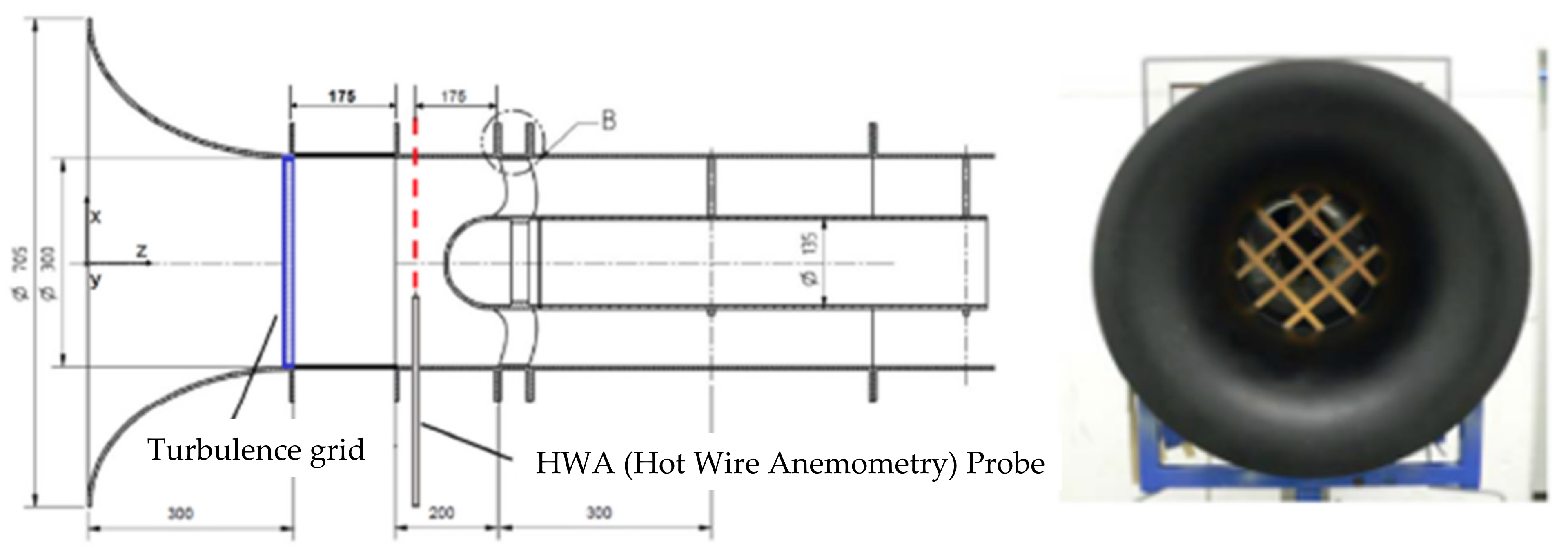
11], which can also be referred to for the measurement setup. In the experiment, an axial fan with a diameter of 300 mm and a rotational speed of 3000 rpm is placed in a duct, sucking air from a semi-anechoic chamber over a comparatively coarse turbulence grid. A schematic of the experimental setup is shown in
Figure 1.
The inflow field for the fan after the nozzle and the turbulence grid is measured by a hot wire probe located 175 mm in front of the leading edge of the fan. In addition, the pressure on the blade surfaces is measured by pressure sensors on the suction and pressure sides of the blades. Here, on 2 blades of the fan 7 pressure sensors were applied on the suction side of one and on the pressure side of the other blade. An additional pressure sensor was installed on the tip gap surface. The signal from the pressure sensors is transferred through channels, which are filled up with a paste, on the opposing blade side to the hub and transmitted to the shaft by sliding contact. The pressure sensors were individually calibrated using a white noise signal.
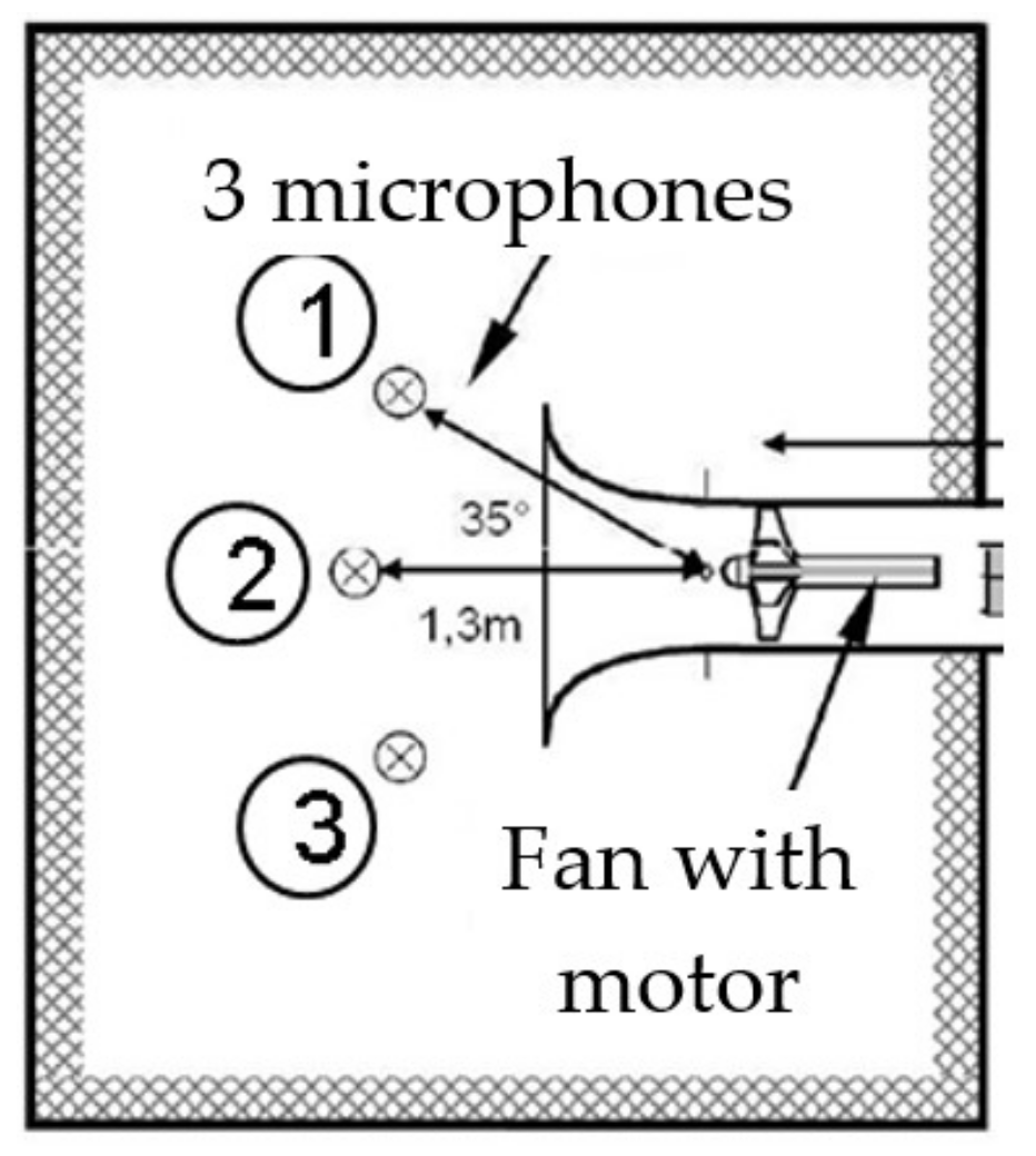
The acoustics are recorded by three upstream microphones placed in the semi-anechoic chamber (
Figure 2) and one microphone in the duct after the fan. For the comparison in this paper, only the microphones on the suction side (semi-anechoic chamber) are used.
3. Simulation Setup
This experiment was selected for the test because it features a turbulent inflow condition for a fan which can still be resolved with a scale-resolving simulation, thereby providing an additional reference for the simulation with turbulent reconstruction.
The basis for all acoustic simulations in this work is a RANS-Simulation of the entire simulation domain, which can be seen in
Figure 3 for the LES setup. The grid resolution of this steady-state simulation is the same as for the scale-resolving aeroacoustic calculations. A polyhedral mesh with approximately 60 million cells was used. The rotation of the fan is realized by the moving reference frame (MRF) method in StarCCM+. The turbulence was calculated using the k-ε realizable model.
The scale-resolving simulation was set up as a compressible simulation in StarCCM+. The propagation of the turbulence generated by the grid to the fan was ensured by at least two cells per turbulent length scale, which has proven sufficient in a previous investigation [
5]. In this transient simulation, the rotation of the fan was realized using the rigid body motion (RBM) method with sliding interfaces. The turbulent boundary layer was resolved, ensuring the dimensionless wall normal distance (N+, Y+) below 1 and a dimensionless resolution in the tangential direction (T+) below 200 in the entire domain leading to the aforementioned approximately 60 million cells. The deployed LES with WALE (Wall-Adapting Local Eddy-viscosity) subgrid-scale (SGS) model typically requires T+ values below 40 for a proper resolution of the boundary layer. However, it was shown that for the acoustics of fans, this setup is sufficient [
1,
5].
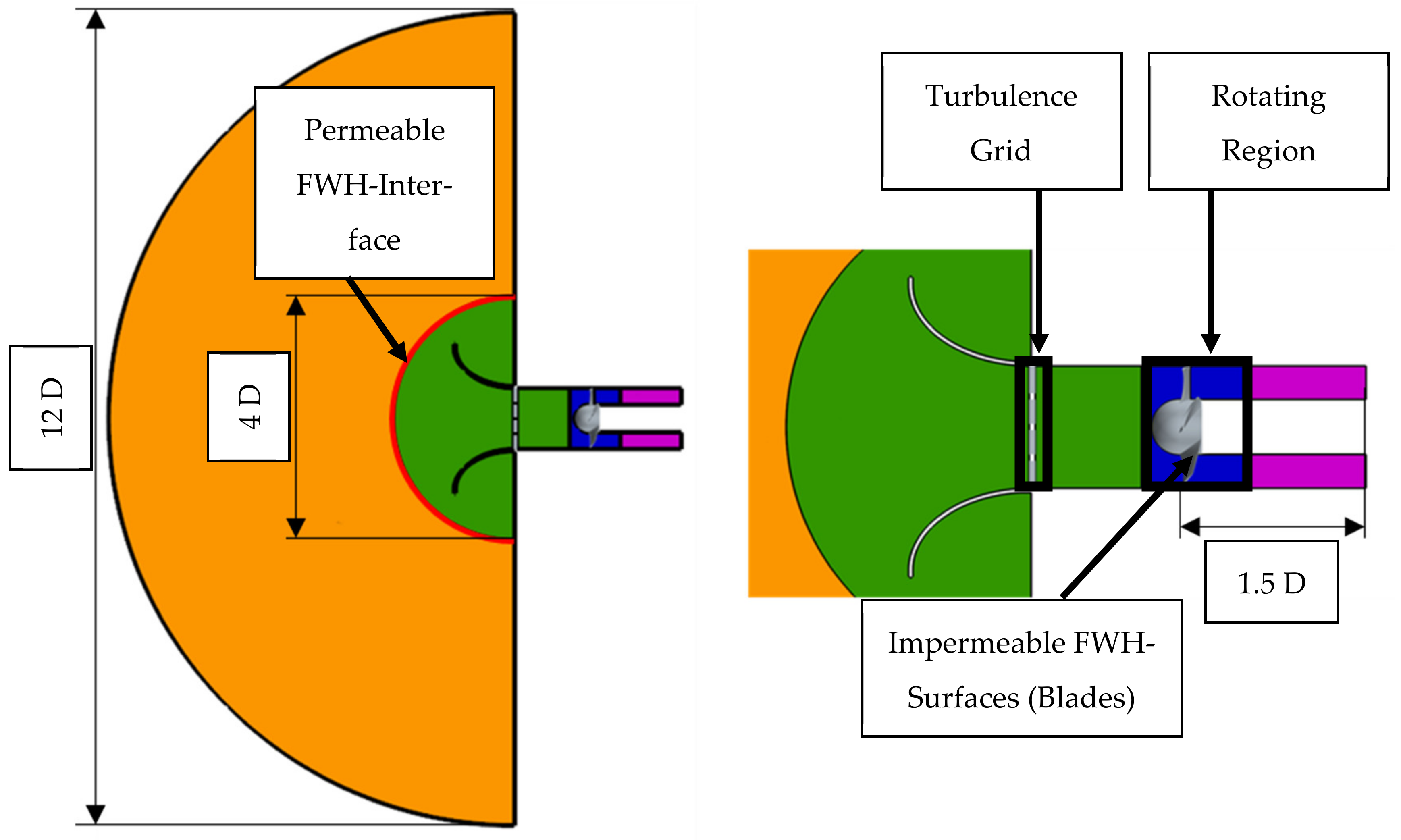
Acoustic waves of frequencies up to 3000 Hz are spatially resolved with 20 points per wavelength (PPW) up to a permeable interface in front of the nozzle. The acoustics for the microphones in the semi-anechoic chamber was calculated using the Ffowcs-Williams and Hawkings (FWH) model directly from the fan blades as well as from the permeable surface in front of the nozzle using Farassat A1 formulation. In order to avoid reflections at the boundaries, the inlet and outlet sections are implemented as non-reflecting “Free-Stream” boundary conditions. In addition, on the outlet, an Acoustic Suppression Zone (ASZ) with a thickness of 0.5 D (diameter of the fan) is applied.
Figure 3 shows a schematic view of the calculation domain.
The simulation is carried out by first calculating three fan revolutions with a comparably coarse timestep. Afterward, the acoustic evaluation of 2 additional revolutions with FWH is started using a smaller timestep of Δt = 5 × 10⁻⁶ s (Δt < Period duration at 3000 Hz divided by 30), ensuring the temporal acoustic resolution up to 3000 Hz.
For the simulation with turbulence reconstruction, the domain used for the previous simulations is reduced. The inlet is now located 175 mm in front of the leading edge (the position of the hot wire measurements in the experiment). Since in the reduced simulation domain, the geometry is either rotating or rotationally symmetric, in contrast to the geometric setup of the full model, the entire domain is realized as rotating using the RBM method. The grid resolution is the same as for the scale-resolving simulation of the entire domain. Due to the reduced simulation domain, all structures upstream of the new inlet location (e.g., turbulence grid and nozzle) are not represented by the grid, leading to a polyhedral mesh of approximately 40 million cells. The transient and acoustic setup is the same as for the full model simulation. However, due to the reduced domain, only the acoustic propagation directly from the fan blades to the microphones in the semi-anechoic chamber via FWH can be considered.
As a basis for the turbulence reconstruction with the FRPM, the RANS simulation, which was used to calculate the initial flow field for the LES of the entire domain, is used. To perform the turbulence reconstruction, a volumetric section (patch) of the mean flow profile and the statistic turbulence properties are extracted from this RANS simulation and provided as input for the FRPM. The reconstruction in the FRPM is carried out on a cartesian mesh. The FRPM patch is centered around the location of the new inlet (0.175 m) upstream of the fan leading edge with a thickness of 5 cm, which is more than three times the maximal turbulent length scale in this section. The FRPM uses a volumetric mesh for the reconstruction in order to ensure a full divergence-free flow field for the fluctuations. The spatial resolution of this mesh is the same as in the polyhedral mesh in StarCCM+, with two cells per minimal turbulent length scale on the patch. For the reconstruction, two particles per cell were used to realize fluctuations based on a Gaussian distribution. The transient turbulent fluctuations reconstructed by the FRPM are then added to the steady-state flow profile of the RANS simulation. This disturbed flow field is then used in the “Free Stream” boundary condition at the inlet. Two different approaches were developed to include the transient profile for the fluctuations. In the first approach, the fluctuations have to be created a priori to the scale-resolving simulation. For the second approach, a one-way coupling between StarCCM+ and the FRPM was realized to allow the reconstruction of the turbulent fluctuations parallel to the LES. In the present work, the fluctuations are created prior to the scale-resolving simulation since this approach is easier to implement and provides a more stable simulation setup.
Figure 4 shows the process of turbulence reconstruction for this case.
4. Aerodynamic Results
The turbulence reconstruction is based on the RANS simulation, which was also used to initialize the scale-resolving simulation of the full model. As already observed in [
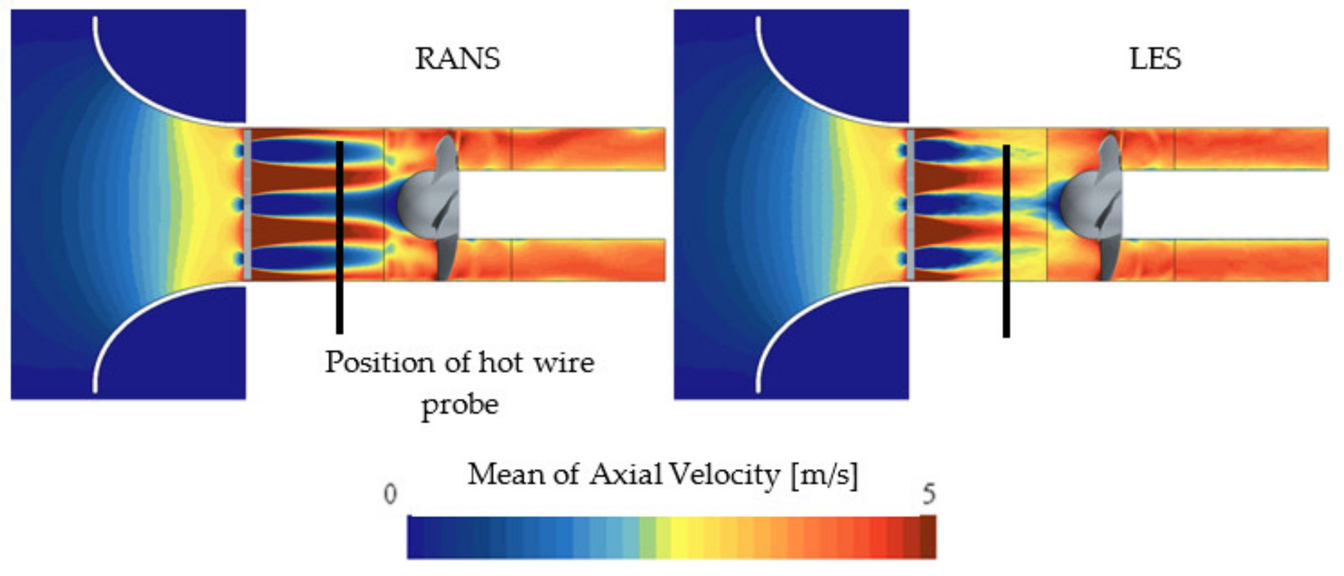
5], the flow field of RANS and LES differ in the structure of the wakes of the turbulence grid. This can also be seen in
Figure 5.
The different structures of the turbulence can also be seen in the comparison to the measurements with the hot wire probe 175 mm in front of the fan, shown in
Figure 6.
In contrast to the measurement, the wakes can be seen in the profiles of the axial velocity for both simulations (RANS and LES). However, in the RANS profile, the structure of the wakes is more clearly visible. Along with the RMS values of the fluctuations (right diagram in
Figure 6), it can be seen that, despite the mean velocity profile, the evaluation time for the fluctuations is not sufficient. Similar behavior of the wakes was also seen in the highly resolved LES by Moghadam et al. [
8]. Nevertheless, previous investigations [
1,
5] showed that, despite differences in aerodynamics, good acoustic results could be obtained with the selected evaluation time and grid resolution. In the RANS velocity and fluctuating profile, as already observed in [
5], the wakes of the turbulence grid are more pronounced compared to LES and measurement. This can be explained by the modeled isotropic turbulence in the RANS approach, since the RMS value was calculated based on the turbulent kinetic energy.
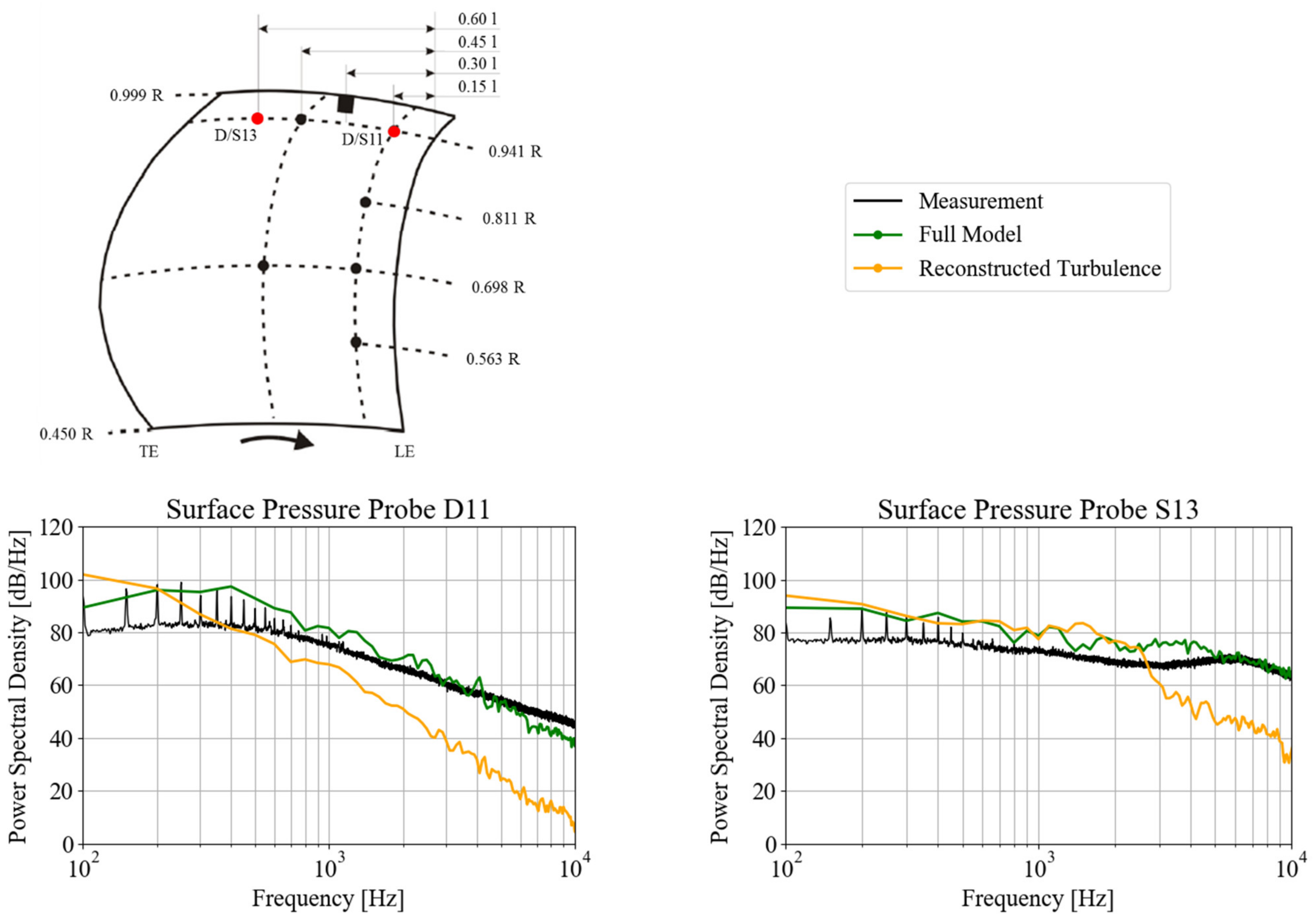
In addition to the hot wire probes, the pressure on the blade’s surfaces can also be compared to the measurements. In
Figure 7, the spectra of the measured surface pressure are compared to the full model simulation and the simulation with reconstructed turbulence.
The surface pressure in the full model simulation shows, for the most part of the spectrum, higher levels compared to the measurement. This can be an effect of the insufficient surface resolution in the presented LES. It can be seen that, especially close to the leading edge on the suction and pressure side, the pressure profile of the reconstructed turbulence shows a significantly faster decay. Close to the trailing edge, the pressure fluctuations of the full model and the reconstructed turbulence are in good agreement, up to ~2500 Hz. For higher frequencies, the pressure signal for the reconstructed turbulence shows significantly lower levels. In the FRPM, a Gaussian spectrum, calibrated with the turbulent kinetic energy and the turbulent length scale of the RANS simulation, is assumed for the reconstruction of the turbulence. The turbulent length scale is dominated by the large turbulent structures of the flow. Therefore, only the part of the turbulent spectrum, which is located around the turbulent length scale, is reconstructed. Small-scale fluctuations at higher frequencies are neglected in the reconstruction leading to an unphysical shape of the energy distribution. This is most likely the reason for the differences found in the pressure spectra.
Previous investigations [
5] showed that, by focusing the reconstruction on the large-scale turbulence based on the RANS mean flow yields good acoustic results compared to reference simulations and measurements. Therefore, it might be assumed that, despite the differences seen for the flow field, good acoustic results can be obtained with the turbulence reconstruction method.
5. Acoustic Results
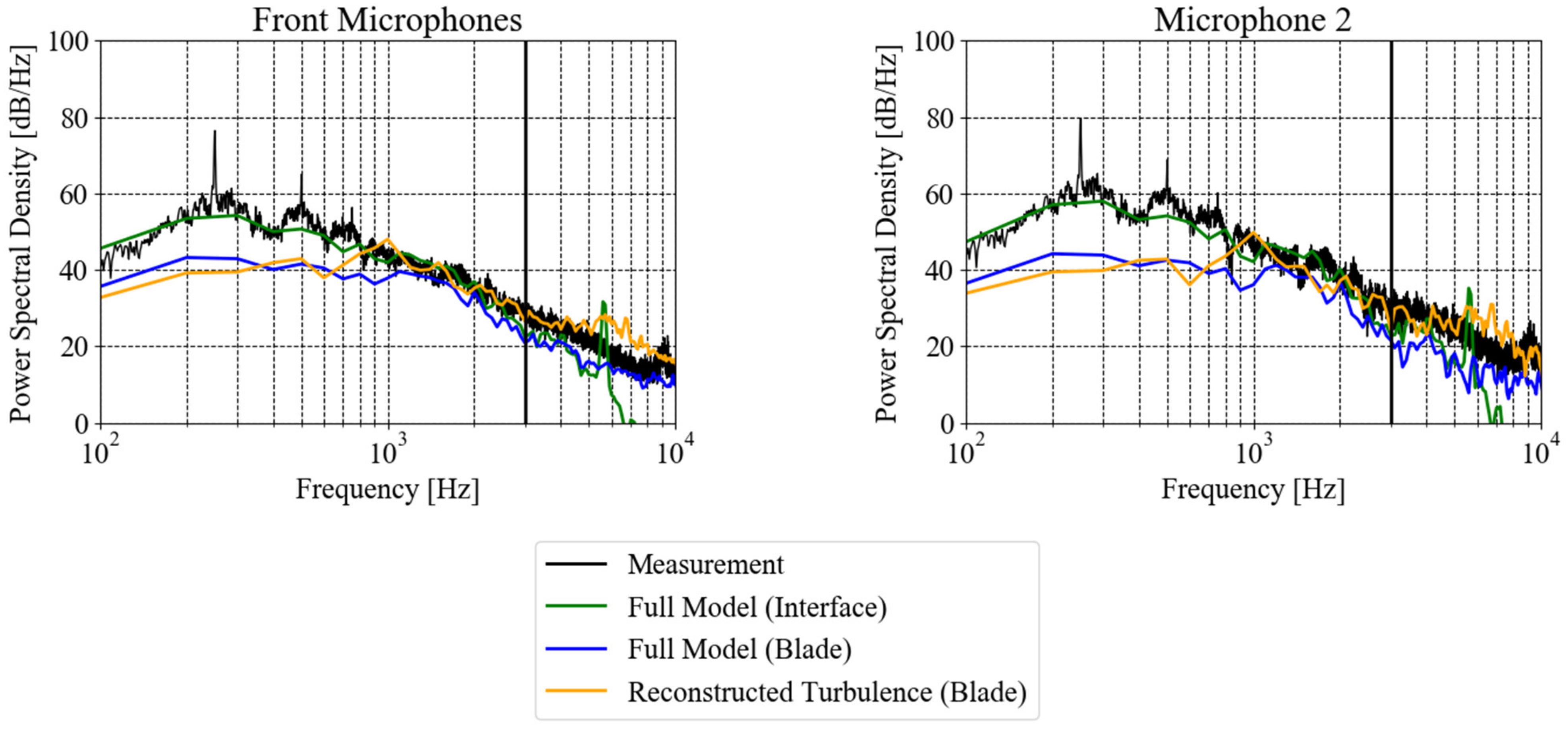
In the full model simulation, the acoustic results in the three microphones in the semi-anechoic chamber can be obtained by propagation using FWH either from the permeable surface or the direct propagation from the fan blades (
Figure 3). In the simulation with reconstructed turbulence due to the reduced simulation domain, only the propagation directly from the fan blades is possible. The average of the acoustic spectra in all three microphones in the semi-anechoic chamber (front) and separately the microphone on the axis (microphone 2) can be found in
Figure 8.
The result based on the propagation from the permeable surface shows a very good agreement with the experimental values. In comparison to the propagation from the blades, the effect of the duct and the nozzle on the acoustic spectrum is clearly visible for frequencies below 1000 Hz. For frequencies above 1000 Hz, the shape of the spectrum and the levels are in good agreement between the different propagation methods.
The reference for the simulation with turbulent reconstruction is the propagation from the fan blades in the full model simulation. The shape of the spectrum and the levels are in close comparison. There are slight differences at 1000 Hz and at higher frequencies. The additional noise at higher frequencies might be an effect of the neglect of small, turbulent fluctuations in the Gaussian spectrum in the turbulence reconstruction method.
Despite the differences in the aerodynamics shown in the previous section, it is possible to correctly predict the effect of the inflow turbulence on the acoustics of the fan by the presented turbulence reconstruction method. In contrast to a heat-exchanger application, the resolution of the turbulence grid in this setup requires a comparably small amount of computational resources.
Due to the short evaluation time, a resolution of the tonal components of the spectra is not possible.
6. Periodic Simulations
To further reduce the computational effort needed to predict the effect of inflow turbulence on the ducted fan, further reduction techniques are investigated. As shown in previous studies [
1,
8], it is possible to exploit the periodicity of the fan geometry in the simulation without inflow turbulence. For the full model approach, this is not possible since the periodicity of the turbulence grid and the fan are not the same (1/5th periodicity for the fan and 1/4th periodicity of the turbulence grid). In the simulation setup with reconstructed turbulence, however, the turbulence grid is no longer part of the simulation domain. Therefore, a new mesh was created, featuring only one blade in a periodic segment. The setups for the full and periodic model for the turbulence reconstruction simulations are displayed in
Figure 9.
Due to the exploitation of the periodicity of the fan geometry, a significant reduction in the cell count can be achieved. Starting from ~60 million cells for the full model (fan and turbulence grid), the cell count is reduced to ~8.6 million for the periodic turbulence reconstruction simulation without the turbulence grid.
For the periodic model, however, it is not possible to directly use the mean flow provided by the precursor RANS, as specified in
Figure 4. The mean flow still shows the structure of the grid, which is of 1/4th periodicity. Using this inflow would lead to unphysical fluctuations in the periodic aeroacoustic simulation. Using the circumferential mean of the RANS flow field and the turbulent fluctuations generated based on the original mean flow, no unphysical fluctuation could be observed in the frequency region of interest. Since it is currently not possible to reconstruct the turbulence in a circumferential periodic domain in the FRPM, the same region as for the full model turbulence reconstruction was used. The profiles used for the mean flow and the turbulence reconstruction are shown in
Figure 10.
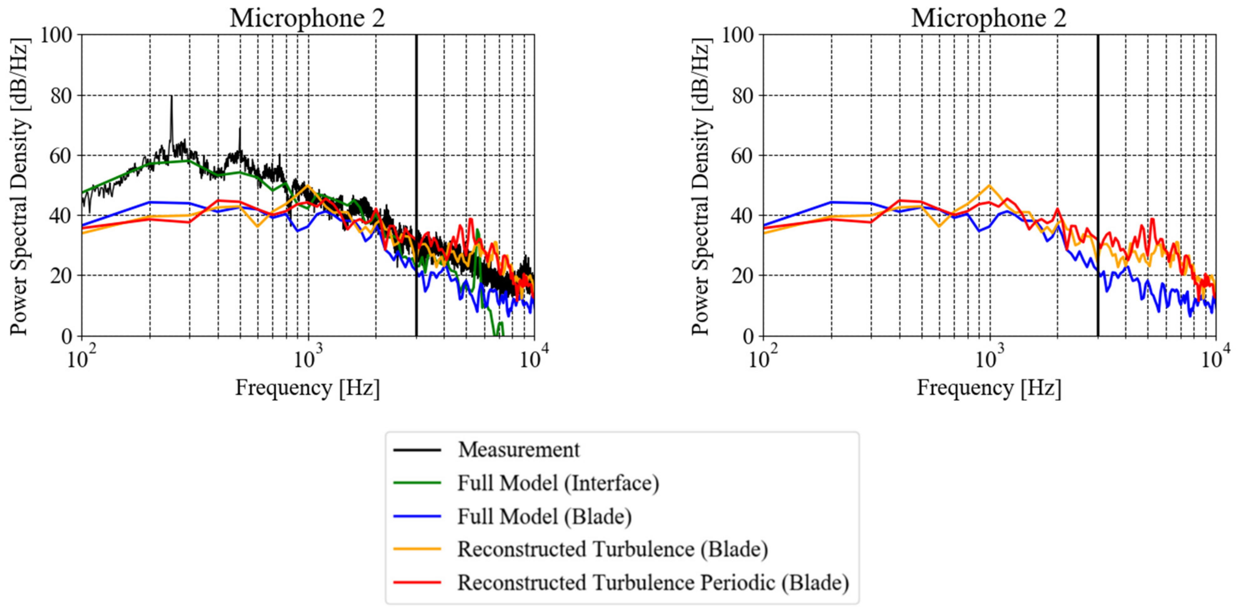
The acoustic results for microphone two can be seen in
Figure 11. The signal for the periodic model is shifted by
(5 representing the number of blades of the fan) account for coherent sound sources on the axis. Here only the microphone on the axis is shown due to the ongoing investigations to account for the effect of coherent sound sources for off-axis microphones (Lucius et al. [
13]).
The acoustic spectrum from the periodic simulation with reconstructed turbulence matches the reference simulation and is also in good agreement with the full model simulation with reconstructed turbulence. For higher frequencies, additional fluctuations can be observed, which can be accounted for by the generation of the synthetic turbulence and the periodic model itself. For the spectrum at low frequencies (f < 1 000 Hz), it is important to use the original RANS flow field for the turbulence reconstruction. If the circumferential mean of the flow field is also used for the turbulence reconstruction, significantly lower levels are observed in this frequency region.
7. Conclusions
In this paper, an approach to reduce the computational effort for the aeroacoustic simulation of fans by reconstructing the turbulence generated by geometric features upstream of the fan is presented. The approach was applied to a benchmark case of an axial fan in a duct with an upstream turbulence grid.
For this approach, the statistical turbulence information from a precursor RANS was reconstructed using the FRPM-Tool, developed at the DLR in Braunschweig, and used as an inlet boundary condition of a scale-resolving aeroacoustic simulation of the fan. The results were compared to the experimental finding and an aeroacoustic simulation of the entire setup (fan + turbulence grid). Additionally, an approach was presented to further reduce the computational effort for acoustic prediction by exploiting the periodicity of the geometry.
The aerodynamic comparison showed that there are differences in the mean flow field and the turbulent properties of the RANS simulation compared to the experiment and the reference LES. Furthermore, the pressure signals on the fan blade surface partially show significant differences between the simulation with reconstructed turbulence and the reference simulation of the entire setup. Despite these differences, a good agreement between the acoustic spectra of the simulations with reconstructed turbulence and the reference simulations was found. The reference spectra from the experiments could not be reproduced with the turbulence reconstructing simulations due to the reduced computational domain. With the turbulence reconstruction and the exploitation of the periodicity of the geometry, it is possible to significantly reduce (up to a factor of 6) the computational effort of aeroacoustic simulations with inflow turbulence.
The simulations show that with the turbulence reconstruction method and the exploitation of periodicity in the geometric setup, it is possible to predict the aeroacoustic behavior of the fan in comparison to simulations of the entire setup. Especially for the typical application of fans in combination with heat exchangers, this method seems promising to be able to capture the effect of the inflow turbulence on the fans’ acoustics, which is currently not economically possible. For the development of new generations of fans with improved acoustic behavior under disturbed inflow conditions, this approach can be a valuable asset. If detailed information in microphones upstream of the suction side is the target of the investigation, an acoustic propagation code can be used in addition to the proposed method.


