Two-Dimensional Model for Consolidation-Induced Solute Transport in an Unsaturated Porous Medium

Abstract

Solute transport through porous media is usually described by well-established conventional transport models with the ability to account for advection, dispersion, and sorption. In this study, we further extend our previous one-dimensional model for solute transport in an unsaturated porous medium to two dimensions. The present model is based on a small-strain approach. The proposed model is validated with previous work. Both homogeneous landfill and pointed landfill conditions are considered. A detailed parametric study shows the differences between the present model and previous one-dimensional model.

1. Introduction

Most conventional models for solute transport in porous media were developed based on the advection–dispersion equation (ADE) using different approaches [1,2,3,4,5]. These studies were based on the assumption of a rigid porous medium in which the volume of the porous medium does not change. Therefore, the advective flow was usually induced by external hydraulic gradient (groundwater flow, rainfall infiltration, etc.). Since the excess pore pressure dissipation produces a transient advective flux of contaminant, which has a strong influence on overall flux [6], consideration of coupled flow and deformation in the consolidation process may be significant in the prediction of the solute transport in a porous medium [7,8,9].

Based on Terzaghi [10]’s one-dimensional (1D) consolidation theory and ADE, numerous studies considered consolidation-induced solute transport in a porous medium [7,8]. These studies consider saturated porous media. Recently, Zhang et al. [9] further developed a 1D small-strain model for a homogeneous unsaturated porous medium, which was further extended to layered media [11].

Note that the aforementioned models were limited to 1D. Based on the piece-wise method, Fox and Berles [12] and Fox [13] conducted a series of theories and performed an experimental test to evaluate their models. Considering a 1D consolidation [12] and 2D solute transport scheme, [13] developed a coupled finite-strain model for saturated porous media named CST1 to include advection, dispersion in both directions, the first-order decay and linear equilibrium adsorption. However, the above investigations were limited to saturated porous media.

In this short communication, we will present the two-dimensional (2D) model for solute transport in an unsaturated porous medium. The theoretical formulation for the 2D model will be outlined first and validated with the existing models. Then, a parametric study will be presented to show the differences between 2D and 1D models.

2. Theoretical Model

In this section, the mathematical formulations of the 2D consolidation-induced solute transport model will be outlined. The present model includes two sub-models: a consolidation sub-model and a solute transport sub-model.

One of the novel contributions of this communication is the development of a two-dimensional model for solute transport in an unsaturated deformable porous medium. In the previous one-dimensional model [7,8,9,14], only the soil deformation in the vertical direction is considered and the solute transport is limited to the vertical direction. In real environments, both soil deformation and solute transport are multi-directional, i.e, two-dimensional or three-dimensional, depending on the loading and dimension of the landfill sites. In this situation, the conventional 1D model cannot fully describe the physical process. To show the difference between the 2D and 1D models, we outline the governing equations for the 1D model in Section 2.4 and Section 2.5 for comparison with the present model.

Another novel contribution of this study is the comparison of the unsaturated porous model with the previous 2D model for saturated porous media [12,13,15], which integrated 1D consolidation with the 2D solute transport model. To demonstrate the difference between saturated and unsaturated models, we outline the governing equations for saturated models for 2D and 1D in Section 2.3 and Section 2.5 for comparison with the present model.

2.1. Two-Dimensional Consolidation Model

In the present model, the small strain 2D consolidation theory was adopted, in which the soil is elastically deformed and excess pore pressure ($p^e$) and soil deformations in 2D space (u, w) are calculated simultaneously. Based on the conservation of mass, the 2D consolidation equation can be expressed as [16]:

$$S_{r}n\beta \frac{\partial p^e}{\partial t}+S_r\nabla ·{\mathbf{v}}_s=\frac{1}{{\rho }_{w}g}\nabla ·\left(\mathbf{K}·\nabla p^e\right),$$

(1)

where $\mathbf{K}$ (m/s) refers to the matrix of hydraulic conductivity:

$$\mathbf{K}=\left[\begin{array}{cc}{K}_x& 0\\ 0& K_z\end{array}\right],$$

(2)

in which $K_x$, and $K_z$ denote the hydraulic conductivity in the x- and z-directions, respectively. Note that (1) was originally derived by Biot [17] and modified by Wu [16] for the 2D case.

In (1), ${\mathbf{v}}_{\mathbf{s}}$ (m/s) is the velocity vector of solid particle movement, which can be determined by:

$${\mathbf{v}}_s\equiv \frac{\partial {\mathbf{u}}_s}{\partial t}=\left(\frac{\partial u}{\partial t},\frac{\partial w}{\partial t}\right),$$

(3)

where ${\mathbf{u}}_s$ is the soil displacement vector (m), while u and w are the soil displacements in the x- and z-directions, respectively.

The compressibility of the pore fluid ($\beta$) is defined as: [18]

$$\beta =\frac{S_r}{K_{w0}}+\frac{1-S_r+r_h{S}_r}{P_a+P_0},$$

(4)

in which $K_{w0}$ (Pa) is the pore water bulk modulus (2000 MPa), $r_h$ is the volumetric fraction of dissolved air within pore water, and $P_a$ and $P_0$ (Pa) are the gauge air pressure and the atmospheric pressure ($P_0=$ 100 kPa), respectively.

Substituting (2) and (3) into (1) leads to the final 2D storage equation with respect to the excess pore pressure ($p^e$) and soil deformation field, ${\mathbf{u}}_s\equiv (u,w)$, i.e.,

$$S_{r}n\beta \frac{\partial p^e}{\partial t}+S_r\frac{\partial (\nabla ·{\mathbf{u}}_s)}{\partial t}=\frac{1}{{\rho }_{w}g}\left(K_x\frac{{\partial }^2{p}^e}{\partial x^2}+K_z\frac{{\partial }^2{p}^e}{\partial z^2}\right).$$

(5)

In addition to the storage equation, soil deformation can be calculated through the force balance equations. Herein, the self weight change in the soil matrix due to the drainage of excess flow is considered and applied to the z-direction. The force balance equation written in matrix form is presented as:

$$\nabla ·\left[\begin{array}{cc}{\sigma }_x^{\prime }& {\tau }_{xz}\\ & \\ {\tau }_{zx}& {\sigma }_z^{\prime }\end{array}\right]-\left[\begin{array}{c}0\\ \\ (1-n^0)({\rho }_s-S_r{\rho }_w)g\left(\nabla ·{\mathbf{u}}_s\right)\end{array}\right]=\left[\begin{array}{c}\frac{\partial p^e}{\partial x}\\ \\ \frac{\partial p^e}{\partial z}\end{array}\right],$$

(6)

where ${\sigma }_x^{\prime }$ and ${\sigma }_z^{\prime }$ (N/m${}^2$) are the normal effective stress in the x- and z-directions, and ${\tau }_{xz}$, ${\tau }_{zx}$ (N/m${}^2$) is the shear stress. The soil is assumed to deform in a linear elastic way; hence, Hooke’s law can be adopted to calculate the effective stress tensor. That is,

$$\begin{array}{c}\hfill {\sigma }_x^{\prime }=2G\left(\frac{\partial u}{\partial x}+\frac{\mu (\nabla ·{\mathbf{u}}_s)}{1-2\mu }\right),\end{array}$$

(7a)

$$\begin{array}{c}\hfill {\sigma }_z^{\prime }=2G\left(\frac{\partial w}{\partial z}+\frac{\mu (\nabla ·{\mathbf{u}}_s)}{1-2\mu }\right),\end{array}$$

(7b)

$$\begin{array}{c}\hfill {\tau }_{xz}={\tau }_{zx}=G\left(\frac{\partial u}{\partial z}+\frac{\partial w}{\partial x}\right).\end{array}$$

(7c)

2.2. Two-Dimensional Solute Transport Model

In this section, the 2D solute transport equation is proposed based on the conventional advection–dispersion equation (ADE). The process of soil consolidation is coupled to the theory by adopting the transient flow due to consolidation as the advective flow in ADE. In addition, both temporal and spatial variations in porosity are taken into account.

Considering the solute mass conservation in both fluid and solid phases, and adopting the linear sorption, the coupled solute transport equation is proposed as [16]:

$$\begin{array}{cc}\hfill [S_r{n}^0+& (1-n^0){\rho }_s{K}_d]\frac{\partial c_f}{\partial t}=S_r{n}^0\left(D_x\frac{\partial c_f^2}{\partial x^2}+D_z\frac{\partial c_f^2}{\partial z^2}\right)+S_r{n}^0\left(\frac{\partial D_x}{\partial x}\frac{\partial c_f}{\partial x}+\frac{\partial D_z}{\partial z}\frac{\partial c_f}{\partial z}\right)\hfill \\ \hfill & +S_r(1-n^0)\left[D_x\left(\frac{\partial u^2}{\partial x^2}+\frac{\partial w^2}{\partial x\partial z}\right)\frac{\partial c_f}{\partial x}+D_z\left(\frac{\partial u^2}{\partial x\partial z}+\frac{\partial w^2}{\partial z^2}\right)\frac{\partial c_f}{\partial z}\right]\hfill \\ \hfill & +\frac{1}{{\rho }_{w}g}\left(K_x\frac{\partial p^e}{\partial x}\frac{\partial c_f}{\partial x}+K_z\frac{\partial p^e}{\partial z}\frac{\partial c_f}{\partial z}\right)\hfill \\ \hfill & -\left[S_r{n}^0+(1-n^0){\rho }_s{K}_d\right]\left(\frac{\partial u}{\partial t}\frac{\partial c_f}{\partial x}+\frac{\partial w}{\partial t}\frac{\partial c_f}{\partial z}\right)\hfill \\ \hfill & +S_r{n}^0\beta \frac{\partial p^e}{\partial t}{c}_f+S_r{n}^0\beta \left(\frac{\partial u}{\partial t}\frac{\partial p^e}{\partial x}+\frac{\partial w}{\partial t}\frac{\partial p^e}{\partial z}\right)c_f\hfill \\ \hfill & -\frac{\beta }{{\rho }_{w}g}\left[K_x{\left(\frac{\partial p^e}{\partial x}\right)}^2+K_z{\left(\frac{\partial p^e}{\partial z}\right)}^2\right]c_f,\hfill \end{array}$$

(8)

where $c_f$ represents the solute concentration in fluid phase; $\mathbf{D}$ refers to the matrix of the hydrodynamic dispersion coefficient shown as:

$$\mathbf{D}=\left[\begin{array}{cc}{D}_x& 0\\ 0& D_z\end{array}\right],$$

(9)

where $D_x$ and $D_z$ are the hydrodynamic dispersion coefficients in the x- and z-directions, respectively.

Note that $\mathbf{D}$ and $\mathbf{K}$ are 2 × 2 matrices, whereas $\mathbf{u}$ is a vector. The hydrodynamic dispersion coefficients can be calculated as the sum of molecular diffusion coefficient and dispersion [19]. That is,

$$\begin{array}{c}\hfill D_x={\alpha }_L\frac{{(v_{fx}-v_{sx})}^2}{|{\mathbf{v}}_{\mathbf{d}}|}+{\alpha }_{TV}\frac{{(v_{fz}-v_{sz})}^2}{|{\mathbf{v}}_{\mathbf{d}}|}+D_m,\end{array}$$

(10a)

$$\begin{array}{c}\hfill D_z={\alpha }_L\frac{{(v_{fz}-v_{sz})}^2}{|{\mathbf{v}}_{\mathbf{d}}|}+{\alpha }_{TV}\frac{{(v_{fx}-v_{sx})}^2}{|{\mathbf{v}}_{\mathbf{d}}|}+D_m,\end{array}$$

(10b)

where $v_{fx}$, $v_{fz}$, $v_{sx}$, $v_{sz}$ (m/s) are respectively the portion of flow and solid velocity in the x- and z-directions; ${\alpha }_L$ refers to the longitudinal dispersion coefficient, ${\alpha }_{TV}$ refers to the transverse dispersion in the vertical direction; $D_m$ is the coefficient of molecular diffusion; $|{\mathbf{v}}_{\mathbf{d}}|$ (m/s) refers to the magnitude of the relative velocity between pore fluid and solid particle, which can be determined as:

$${\mathbf{v}}_{\mathbf{d}}=\left[\begin{array}{c}{v}_{fx}-v_{sx}\\ \\ v_{fz}-v_{sz}\end{array}\right]=\frac{1}{{\rho }_{w}g{S}_r{n}^0}\left[\begin{array}{c}-K_x\left(\frac{\partial p^e}{\partial x}\right)\\ \\ -K_z\left(\frac{\partial p^e}{\partial z}\right)\end{array}\right].$$

(11)

In summary, three governing equations in 2D with respect to the field of excess pore pressure (5), soil deformation (6), and solute concentration (8) have been outlined. The first two equations related to the soil consolidation process are fully coupled and need to be solved simultaneously, whereas the last solute transport governing equation is semi-coupled and can be solved utilising the consolidation outcomes.

The above governing equations can be solved using appropriate boundary conditions for various engineering problems, such as the case presented in Section 4 using the FEM software COMSOL Multiphysics [20]. In the COMSOL model, the PDF solver is used to establish both consolidation and solute transport models. First, with the loading profile at the ground surface, the consolidation process will be simulated by solving (5) and (6) for the pore pressures and soil displacements in the soil modulus. With the pore pressures and soil displacements obtained from soil modulus, the concentration of solute transport can be solved in the solute modulus. Both moduli are developed in the COMSOL environment and the variables are linked together.

2.3. Special Case 1: Two-Dimensional Saturated Porous Model

In the present model, a two-dimensional solute transport in an unsaturated porous medium is proposed. A special case occurs for a fully saturated porous medium, in which $S_r=1$ and $\beta \to 0$, according to (4). Then, the governing equations for the present model can be simplified as

$$\frac{\partial (\nabla ·{\mathbf{u}}_s)}{\partial t}=\frac{1}{{\rho }_{w}g}\left(K_x\frac{{\partial }^2{p}^e}{\partial x^2}+K_z\frac{{\partial }^2{p}^e}{\partial z^2}\right).$$

(12)

$$\nabla ·\left[\begin{array}{cc}{\sigma }_x^{\prime }& {\tau }_{xz}\\ & \\ {\tau }_{zx}& {\sigma }_z^{\prime }\end{array}\right]-\left[\begin{array}{c}0\\ \\ (1-n^0)({\rho }_s-{\rho }_w)g\left(\nabla ·{\mathbf{u}}_s\right)\end{array}\right]=\left[\begin{array}{c}\frac{\partial p^e}{\partial x}\\ \\ \frac{\partial p^e}{\partial z}\end{array}\right],$$

(13)

$$\begin{array}{cc}\hfill [n^0+& (1-n^0){\rho }_s{K}_d]\frac{\partial c_f}{\partial t}=n^0\left(D_x\frac{\partial c_f^2}{\partial x^2}+D_z\frac{\partial c_f^2}{\partial z^2}\right)+n^0\left(\frac{\partial D_x}{\partial x}\frac{\partial c_f}{\partial x}+\frac{\partial D_z}{\partial z}\frac{\partial c_f}{\partial z}\right)\hfill \\ \hfill & +(1-n^0)\left[D_x\left(\frac{\partial u^2}{\partial x^2}+\frac{\partial w^2}{\partial x\partial z}\right)\frac{\partial c_f}{\partial x}+D_z\left(\frac{\partial u^2}{\partial x\partial z}+\frac{\partial w^2}{\partial z^2}\right)\frac{\partial c_f}{\partial z}\right]\hfill \\ \hfill & +\frac{1}{{\rho }_{w}g}\left(K_x\frac{\partial p^e}{\partial x}\frac{\partial c_f}{\partial x}+K_z\frac{\partial p^e}{\partial z}\frac{\partial c_f}{\partial z}\right)\hfill \\ \hfill & -\left[n^0+(1-n^0){\rho }_s{K}_d\right]\left(\frac{\partial u}{\partial t}\frac{\partial c_f}{\partial x}+\frac{\partial w}{\partial t}\frac{\partial c_f}{\partial z}\right).\hfill \end{array}$$

(14)

Comparing the above governing equations with the ones outlined in Section 2.1 and Section 2.2, the unsaturated model is much more complicated than a saturated model. Since the soil near the ground surface is commonly unsaturated in real environments, it is necessary to consider an unsaturated porous medium in the simulation of the solute transport in a deformable medium.

2.4. Special Case 2: One-Dimensional Unsaturated Porous Model

The present model can be simplified to a one-dimensional case,

$$S_r{n}^0\beta \frac{\partial p^e}{\partial t}+S_r\frac{{\partial }^{2}w}{\partial t\partial z}=\frac{1}{{\rho }_{w}g}\frac{\partial }{\partial z}\left(K\frac{\partial p^e}{\partial z}\right),$$

(15)

$$G\frac{2(1-\mu )}{(1-2\mu )}\frac{{\partial }^{2}w}{\partial z^2}+(1-n^0)({\rho }_s-{\rho }_w)g\frac{\partial w}{\partial z}=\frac{\partial p^e}{\partial z},$$

(16)

$$\begin{array}{cc}\hfill \left[S_{r}n+(1-n){\rho }_s{K}_d\right]\frac{\partial c_f}{\partial t}=& S_{r}nD\frac{{\partial }^2{c}_f}{\partial z^2}+\frac{\partial c_f}{\partial z}\left\{S_{r}n\frac{\partial D}{\partial z}+S_{r}D(1-n)\frac{{\partial }^{2}w}{\partial z^2}\right.\hfill \\ \hfill & \left.+\frac{K}{{\rho }_{w}g}\frac{\partial p^e}{\partial z}-\left[S_{r}n+(1-n){\rho }_s{K}_d\right]\frac{\partial w}{\partial t}\right\}+S_{r}n\beta \frac{\partial p^e}{\partial t}{c}_f,\hfill \end{array}$$

(17)

identical to the governing equations in Zhang et al. [9].

2.5. Special Case 3: One-Dimensional Saturated Model

Again, the present model can be simplified to a one-dimensional saturated case with $S_r$ = 1 and $\beta \to 0$,

$$n^0\beta \frac{\partial p^e}{\partial t}+\frac{{\partial }^{2}w}{\partial t\partial z}=\frac{1}{{\rho }_{w}g}\frac{\partial }{\partial z}\left(K\frac{\partial p^e}{\partial z}\right),$$

(18)

$$G\frac{2(1-\mu )}{(1-2\mu )}\frac{{\partial }^{2}w}{\partial z^2}+(1-n^0)({\rho }_s-{\rho }_w)g\frac{\partial w}{\partial z}=\frac{\partial p^e}{\partial z},$$

(19)

$$\begin{array}{cc}\hfill \left[n+(1-n){\rho }_s{K}_d\right]\frac{\partial c_f}{\partial t}=& nD\frac{{\partial }^2{c}_f}{\partial z^2}+\frac{\partial c_f}{\partial z}\left\{n\frac{\partial D}{\partial z}+D(1-n)\frac{{\partial }^{2}w}{\partial z^2}\right.\hfill \\ \hfill & \left.+\frac{K}{{\rho }_{w}g}\frac{\partial p^e}{\partial z}-\left[n+(1-n){\rho }_s{K}_d\right]\frac{\partial w}{\partial t}\right\},\hfill \end{array}$$

(20)

identical to the governing equations in the previous model [8].

3. Model Validation

Due to the lack of field measurements and experimental data, the validation of the present model can only be carried out by reproducing and converting the present model from 2D to 1D with regard to the excess pore pressure, settlement and solute concentration with the existing 1D model.

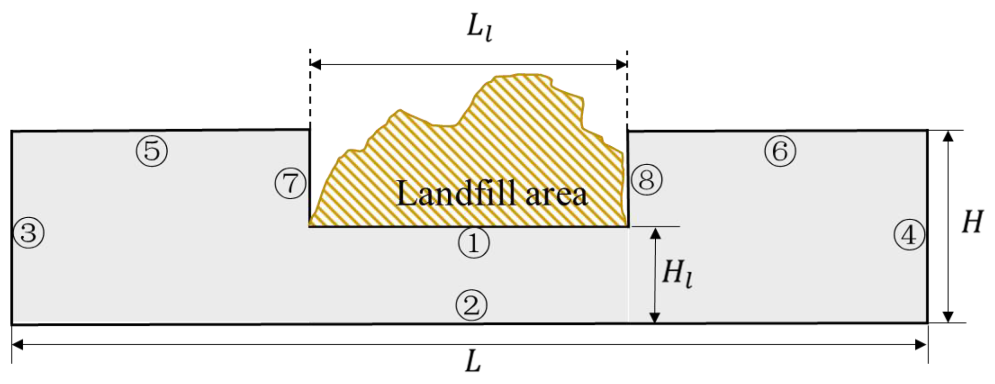
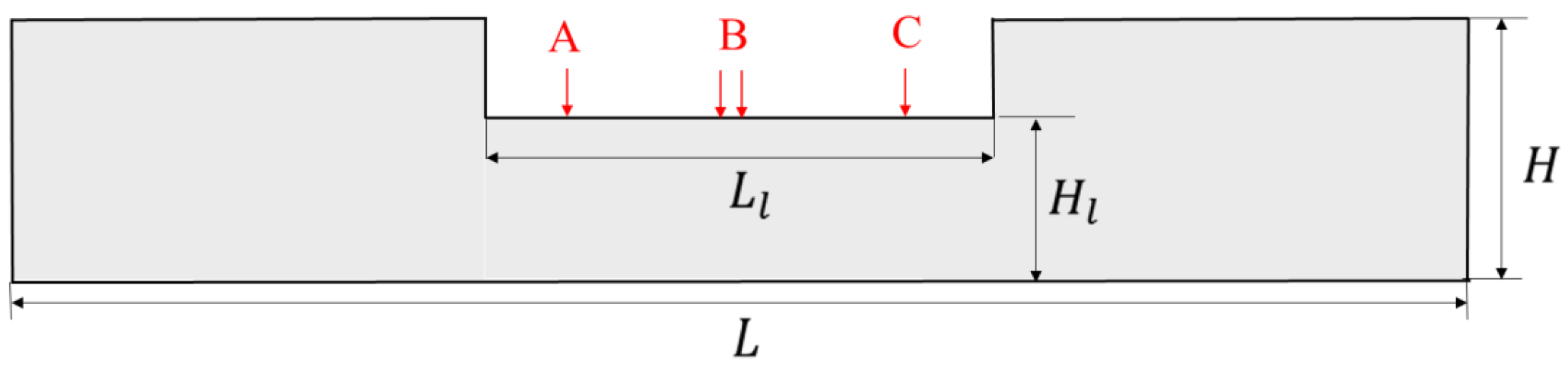
In this section, the developed model was first established in a 2D rectangular domain (Figure 1) under the action of a ramp load; then, the model results extracted from the center vertical cut line were compared with the 1D model results to demonstrate the validity of the developed model. The width ($L_l$) of this 2D domain varied from 1 m to 20 m, while the domain depth ($H_l$) was fixed at 3 m, and origin was located at the bottom left corner.

Boundary conditions (BCs) and initial conditions (ICs) are summarised in

Table 1. Boundary conditions (BCs) and initial condition (ICs) setup for the rectangular domain.

Boundary Index	BC of ${\mathit{p}}^{\mathit{e}}$	BC of $\mathit{u},\mathit{w}$	BC of ${\mathit{c}}_{\mathit{f}}$
1	$\frac{\partial p^e}{\partial z}=0$	$\left[\begin{array}{c}0\\ {\sigma }_z\end{array}\right]=\left[\begin{array}{c}0\\ Q\left(t\right)+p^e\end{array}\right]$	$\frac{\partial c_f}{\partial z}=\frac{D_G}{n^{0}h{D}_m}(c_f-c_0)$
2	$p^e=0$	$\left[\begin{array}{c}u\\ w\end{array}\right]=\left[\begin{array}{c}0\\ 0\end{array}\right]$	$\frac{\partial c_f}{\partial z}=0$
3 & 4	$\frac{\partial p^e}{\partial x}=0$	$u=0$	$\frac{\partial c_f}{\partial x}=0$
IC: $p^e=0$, $\left[\begin{array}{c}u\\ w\end{array}\right]=\left[\begin{array}{c}0\\ 0\end{array}\right]$ and $c_f=0$

. The horizontal Darcy flow is assumed to be impeded at the two lateral boundaries (③ and ➃) where the solute flux is assumed to be zero in the x-direction. Herein, we assume that the soil domain is homogeneous and isotropic, and a uniform load is applied to this domain. The input parameters for computation are given in

Table 2. Parameters for the 2D model validation with the 1D model.

Parameter	Value	Description
$Q\left(t\right)$	Referring to Figure 2	Waste loading
h	0.0015 m	Thickness of geomembrane
${}^{*}{H}_l$	3 m	Depth of soil domain
$L_l$	1 m, 3 m, 5 m, 8 m, 10 m and 20 m	Width of soil domain
$S_r^0$	0.88	Degree of saturation
$n^0$	0.33	Initial porosity
G	$2.75\times {10}^6$ Pa	Shear modulus
$\mu$	0.33	Poisson’s ratio
${}^{*}{K}_x$	$1\times {10}^{-10}$ m/s	Hydraulic conductivity in the x-direction
$K_z$	$1\times {10}^{-10}$ m/s	Hydraulic conductivity in the z-direction
${\rho }_w$	$1\times {10}^3$ kg/m${}^3$	Density of the pore fluid,
		varied due to fluid compressibility
${\rho }_s$	$2.6\times {10}^3$ kg/m${}^3$	Density of the solid phase
$K_d$	0	Partitioning coefficient
$r_h$	0.02 m	Volumetric fraction of dissolved air
		within pore water
$D_G$	$1.5\times {10}^{-4}$ m${}^2$/s	Mass transfer coefficient of geomembrane
$D_m$	$5\times {10}^{-9}$ m${}^2$/s	Molecular diffusion coefficient in the clay
${\alpha }_L$	0.1 m	Longitudinal dispersion coefficient
${}^{*}{\alpha }_T$	0.1 m	Transverse dispersion coefficient
$c_0$	0.1 kg/m${}^3$	Reference solute concentration

Note 1: The symbol * indicates that the parameter is only applied in the 2D model, while the rest of the parameters remain same in both models. Note 2: Total of six 2D models were computed with various $H_l$ as listed.

.

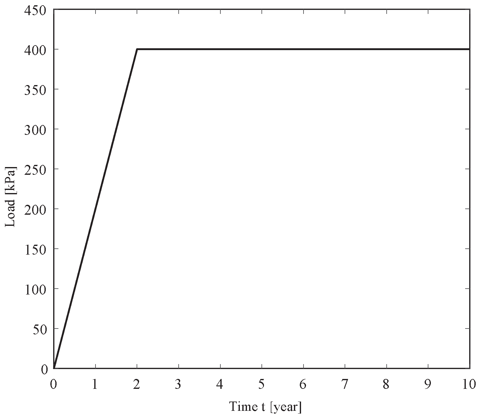
In the comparison with the 1D model [9], a landfill with one leachate collection system was assumed to be constructed on the top of a soil layer (Figure 2). The contaminant migration through the soil layer beneath the landfill is evaluated. As shown in Figure 2, the external load (Q) continues to increase at a rate of 200 kPa annually for two years and remains constant at 400 kPa until the end of simulation period.

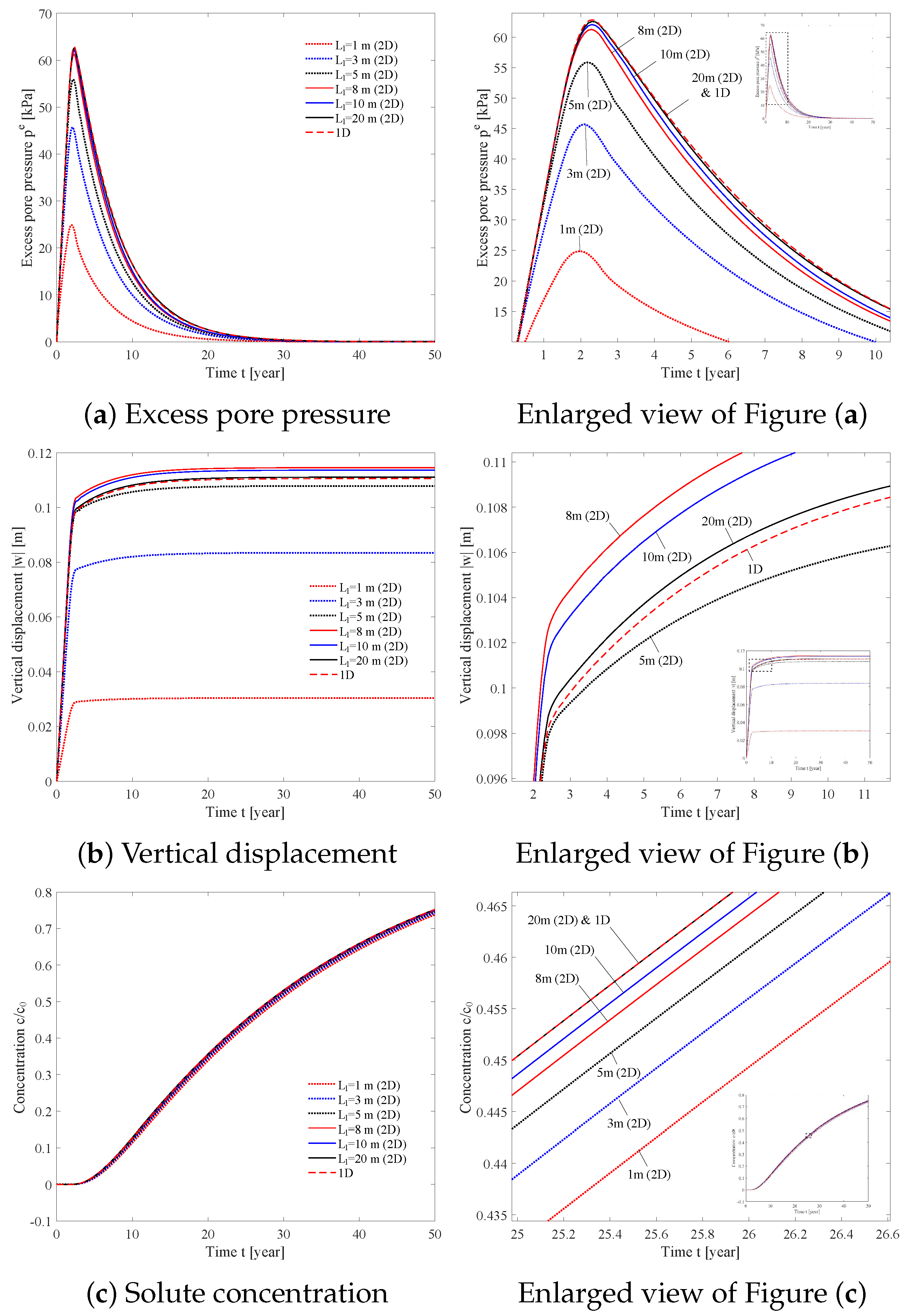
In the 1D model [9], a fully coupled theory was used to describe the consolidation-induced solute transport in the vertical direction while the mass conservation of pore fluid and solute flux along the z-direction was satisfied. Recall the proposed 2D model where drainage is prohibited at the lateral boundaries, and the excess pore fluid can only drains from the bottom. This means that if the computational domain is wide enough (relative to the depth), the results along center vertical cut line from 2D model should be same as the 1D result. To prove this, 2D simulations were conducted for varied length of the computational domain while keeping the depth of the domain constant at 3 m. Figure 3 shows the evolution of excess pore pressure, vertical displacement as well as solute concentration versus time at either the inlet point or the outlet point along the the center vertical cut line. To be more specific, a higher excess pore pressure and faster contaminant migration could be observed as the domain width increased. When $L_l$ was increased to 20 m, the 2D results appeared to be exactly the same as those obtained in the 1D model; the results obtained for $L_l$ = 10 m were also acceptable. Therefore, it has been proven that when the clay layer is thin enough (i.e., $H_l/L_l<<1$), the 1D model is adequate to describe the solute concentration development. However, the 1D model is limited to a homogeneous and isotropic soil environment with uniform loading and contaminant source injection. Additionally, contaminant conditions around the landfill are also meaningful, but could not be addressed by the 1D model [9].

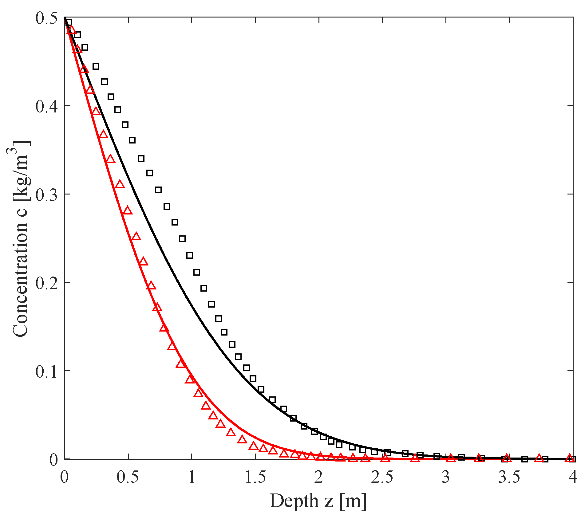
Another model validation was performed by comparing the simulated results with the numerical model developed by Zhang and Fang [15], where a constant loading of 100 kPa was applied to the top surface with linear adsorption. The parameters used for this validation are summarised in

Table 3. Parameters for the validation with Zhang and Fang [15].

Parameter	Value	Description
$Q\left(t\right)$	100 kPa	Constant waste loading
$S_r^0$	1.0	Initial degree of saturation
$n^0$	0.44	Initial porosity
G	$2.6\times {10}^6$ Pa	Shear modulus
$\mu$	0.3	Poisson’s ratio
$K_x$	$1.7\times {10}^{-9}$ m/s	Hydraulic conductivity in x-direction
$K_z$	$1.7\times {10}^{-9}$ m/s	Hydraulic conductivity in z-direction
${\rho }_s$	$2.6\times {10}^3$ kg/m${}^3$	Density of the solid phase
$K_d$	$8.142\times {10}^{-4}$ kg/m	Partitioning coefficient
$D_m$	$6.76\times {10}^{-9}$ m${}^2$/s	Molecular diffusion coefficient in the clay
${\alpha }_L$	0.5 m	Longitudinal dispersion coefficient
${\alpha }_T$	0.05 m	Transverse dispersion coefficient
$c_0$	0.5 kg/m${}^3$	Reference solute concentration

. Note that the Zhang and Fang [15] model only considered a saturated soil with a constant loading. In this validation, the present model was adopted for the case of Zhang and Fang [15].

Figure 4 presents the distribution of solute concentration along a vertical cut line. In general, the results of the proposed model and that of Zhang and Fang [15] show similar trends. Figure 4 indicates that for both models, solutes vertically migrated to the depth of 2 m at year 5 and then spread to 3 m after 10 years. Moreover, the results after 5 years show better agreement between the two models, whereas as the simulation time increases, a less-polluted situation can be observed in the present model. This difference may be caused by the use of an empirical relationship between soil permeability and void ratio in the model of Zhang and Fang [15], which facilitates the development of solute migration in the long-term simulation. Moreover, some of the results in [15] lacked an explanation, such as the cut line locations where the vertical and horizontal distributions of solute concentration were drawn were not specified, and the domain dimensions were not given. However, due to the lack of experimental and field data, the comparison with Zhang and Fang [15] is still presented here as a benchmark validation.

4. Results and Discussions

In this section, a series of numerical examples for consolidation-induced solute transport in an unsaturated porous medium are presented and discussed. The present 2D model is able to describe the consolidation-induced solute transport in both the vertical and horizontal directions. Although the load is applied in the vertical direction, flow and solute migration are allowed in both directions. This section provides two studies to address 2D consolidation-induced solute transport problem. Section 4.1 introduces a simulation of a simplified landfill case with homogeneous and isotropic soil, and the pollution source is assumed to be uniform and existing on all contact surfaces. Following that, with pointed contaminant source, Section 4.2 shows the spread of pollution in the clay liner directly beneath the landfill.

4.1. Homogeneous Soil and Uniform Contaminant Source (2D)

As shown in Figure 5, a sketch of the 2D landfill is proposed. Wastes are dumped into the center landfill area, which leads to a ramp load applied on boundary ①. In this case, drainage is only allowed at the bottom (boundary ②), while the lateral boundaries ③, ⑦, ⑧ and ④ prevent the horizontal flow and the top boundaries (⑤ and ⑥) have zero vertical excess pore pressure gradient. Moreover, in one of the most extreme cases, the volatile source of pollution could diffuse through the geomembrane and spread into the surrounding soil through boundaries ①, ⑦ and ⑧, which are in contact with wastes. The total length of domain (L) is 60 m, and the center landfill area is 20 m long ($L_l$). The depth of the landfill area is 20 m and a compacted clay layer of 3 m ($H_l)$ is located directly beneath the landfill. The remaining parameters are listed in Table 2.

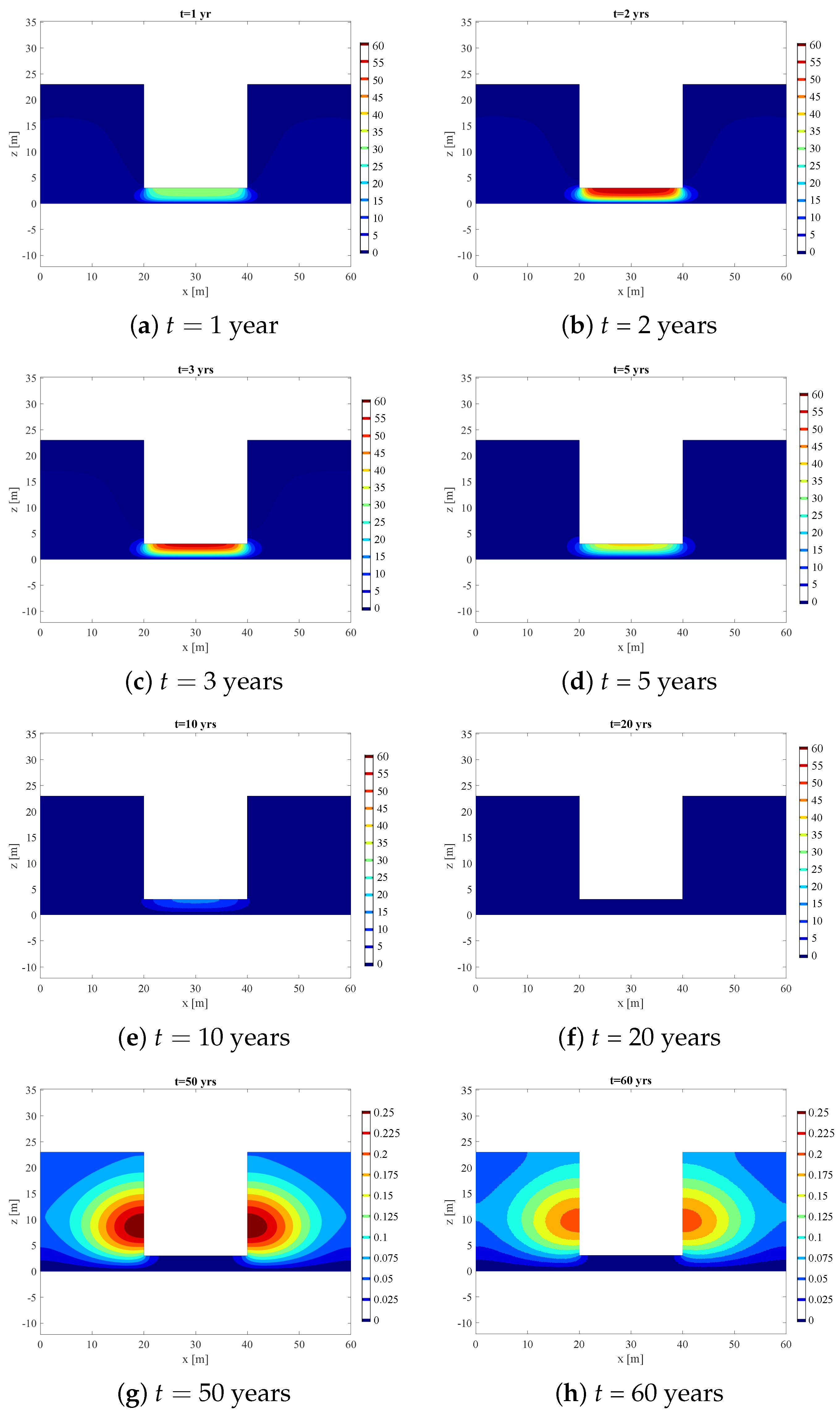
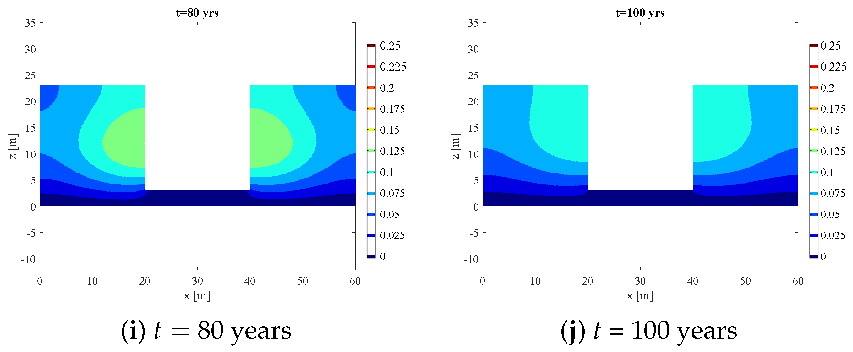
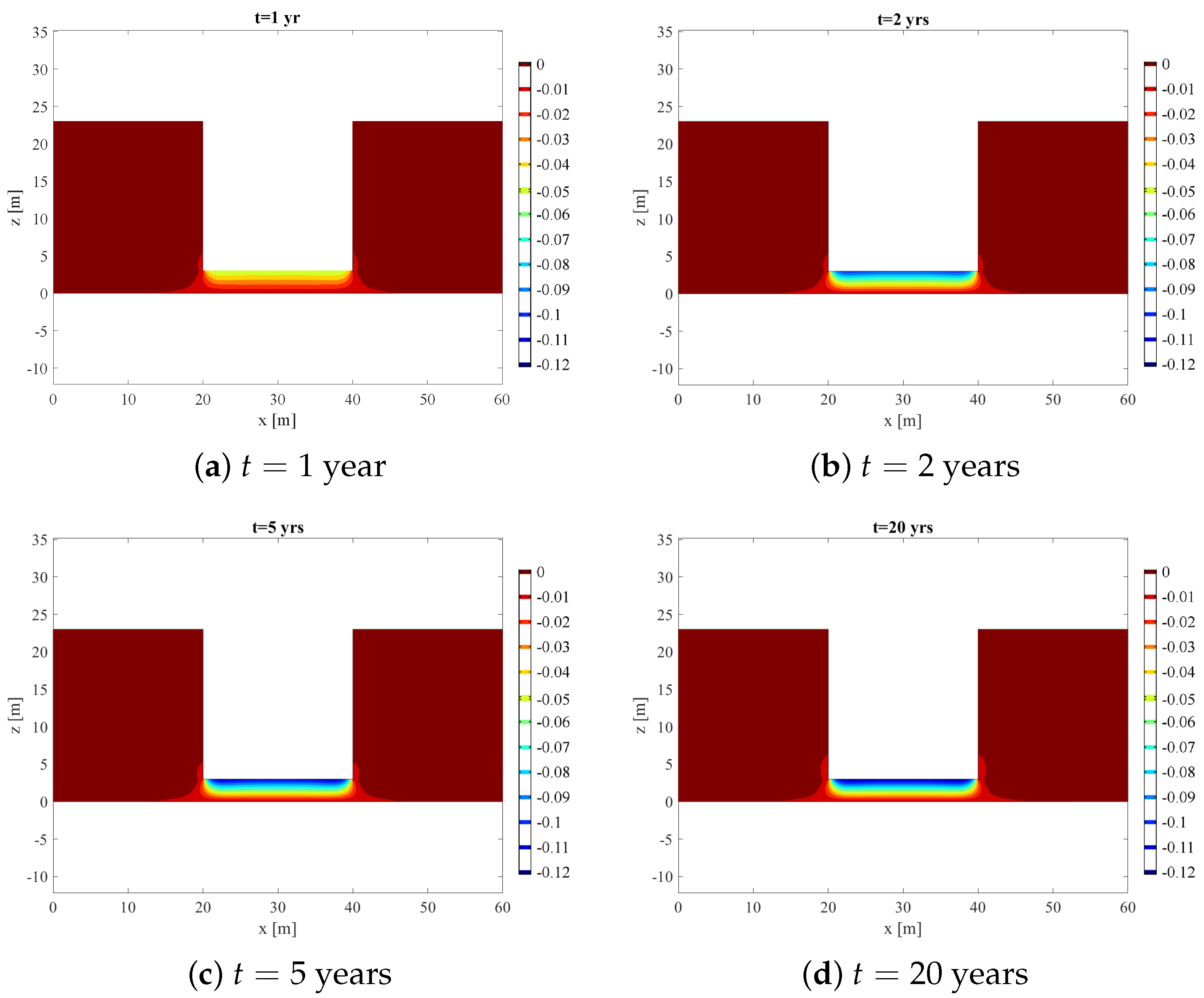
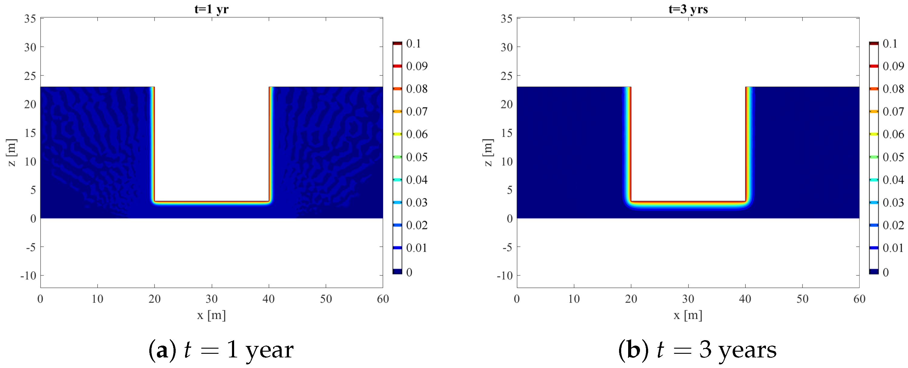
Figure 6 shows the contour plot of excess pore pressure distribution from the 1st year to the 100th year. As shown in the figure, $p^e$ increases from the first to the second year and starts to decrease from the third year. Because the free drainage boundary condition is assumed at the bottom, $p^e$ remains at zero at $z=0$ at all time steps. Furthermore, Figure 6f shows that $p^e$ at 20 years is less than 5 kPa within the entire domain. Although drainage is only allowed at the bottom, pore pressure differences exist in the horizontal direction. Consequently, the transient excess fluid not only flows downward at the center loaded area, but can also flow to the side and enter the surrounding area. To observe the excess pore pressure at the surrounding area, Figure 6g–j are presented with a smaller colour range (0–250 Pa), and Figure 6g–j are plotted for 50 years, 60 years, 80 years and 100 years, respectively. Since $p^e$ can only dissipate from the bottom, it is difficult to dissipate around the surrounding area, but will eventually fully dissipate after sufficient time has passed. As Figure 6j shows, at the end of the 100th year, the highest residual excess pore pressure is only 100 Pa near the top. It is important to point out that the excess pore pressure under the loaded area is already fully dissipated after 20 years, while the surrounding area has some residual $p^e$ left.

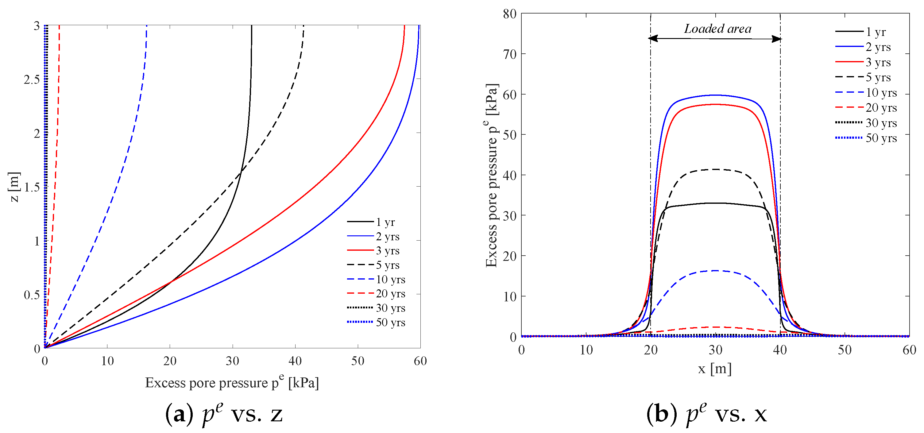
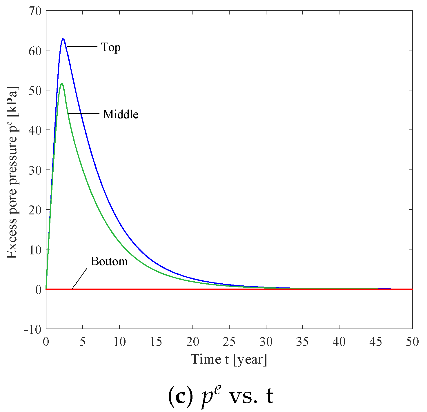
More detailed excess pore pressure progress can be studied from Figure 7. All three subplots focus on the $p^e$ results within the region directly beneath the landfill. The $p^e$ distribution along the vertical cut line plot indicates that pore pressure is the highest at the top surface and then gradually reduces to zero. In the horizontal direction where z = 3 m, $p^e$ coan be detected outside the loaded region ($x=$ 20 m to $x=$ 40 m); driven by the pore pressure differences, the excess pore fluid flows to the surrounding area. Moreover, Figure 7c reveals that $p^e$ has risen sharply and peaks at the level of 62 kPa after around 2.5 years when the external loading reaches its maximum value. After the loading becomes constant, pore pressure starts to dissipate and it takes 30 years to return to 0 at the location of the top point.

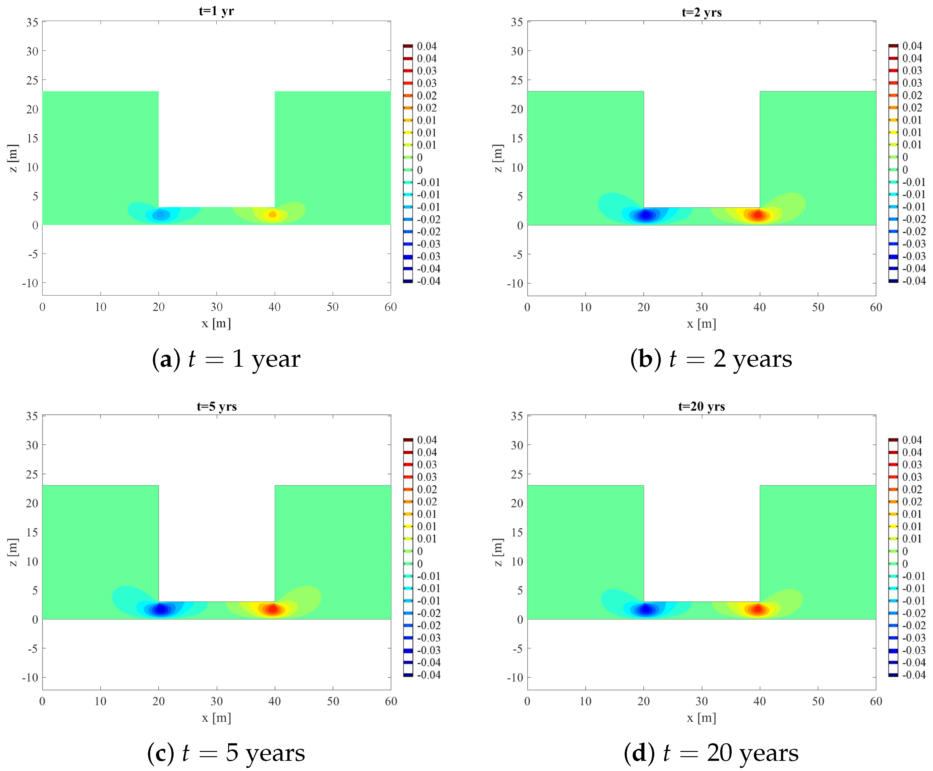
With the ramp loading acting on the clay liner, consolidation results in a soil deformation. Figure 8 and Figure 9 show the distributions of horizontal displacements (u) and vertical displacements (w) at different time steps. The $+/-$ sign denotes the direction of the displacement. Specifically, the largest horizontal displacement is 4 cm in the $-x$ direction at $x=$ 20 m, and 4 cm in the $+x$ direction at $x=$ 40 m. Meanwhile, all vertical displacements are pointing downwards. The horizontal displacement exists near the corner of the landfill, while the vertical displacements are generally uniform beneath the landfill area.

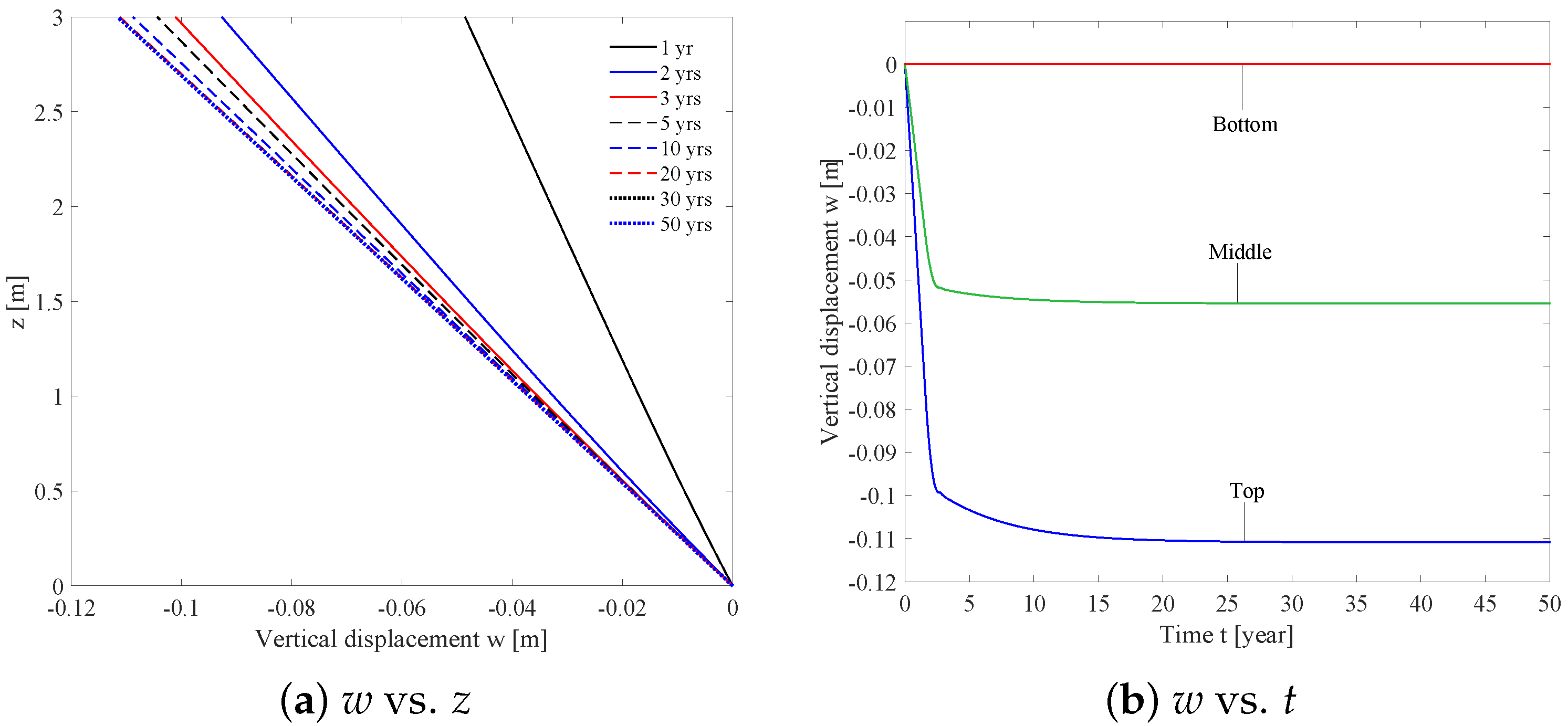
Additionally, Figure 10 presents the vertical and horizontal soil deformation distribution by plotting u and w along the center vertical cut line and horizontal cut line at different locations. Figure 10a demonstrates that the largest vertical displacement occurs on the top of the clay liner. At the first 2 years, the vertical displacement rapidly increases; after reaching the post-loading stage, as excess pore pressure gradually dissipates, w slowly increases until it reaches the final level of 11 cm (Figure 10b. In general, the final state of the horizontal displacement is easier to reach compared with w. Figure 10c reveals that at level $z=$1.5 m, it takes only 2 years to achieve the maximum horizontal displacement value of 3 cm.

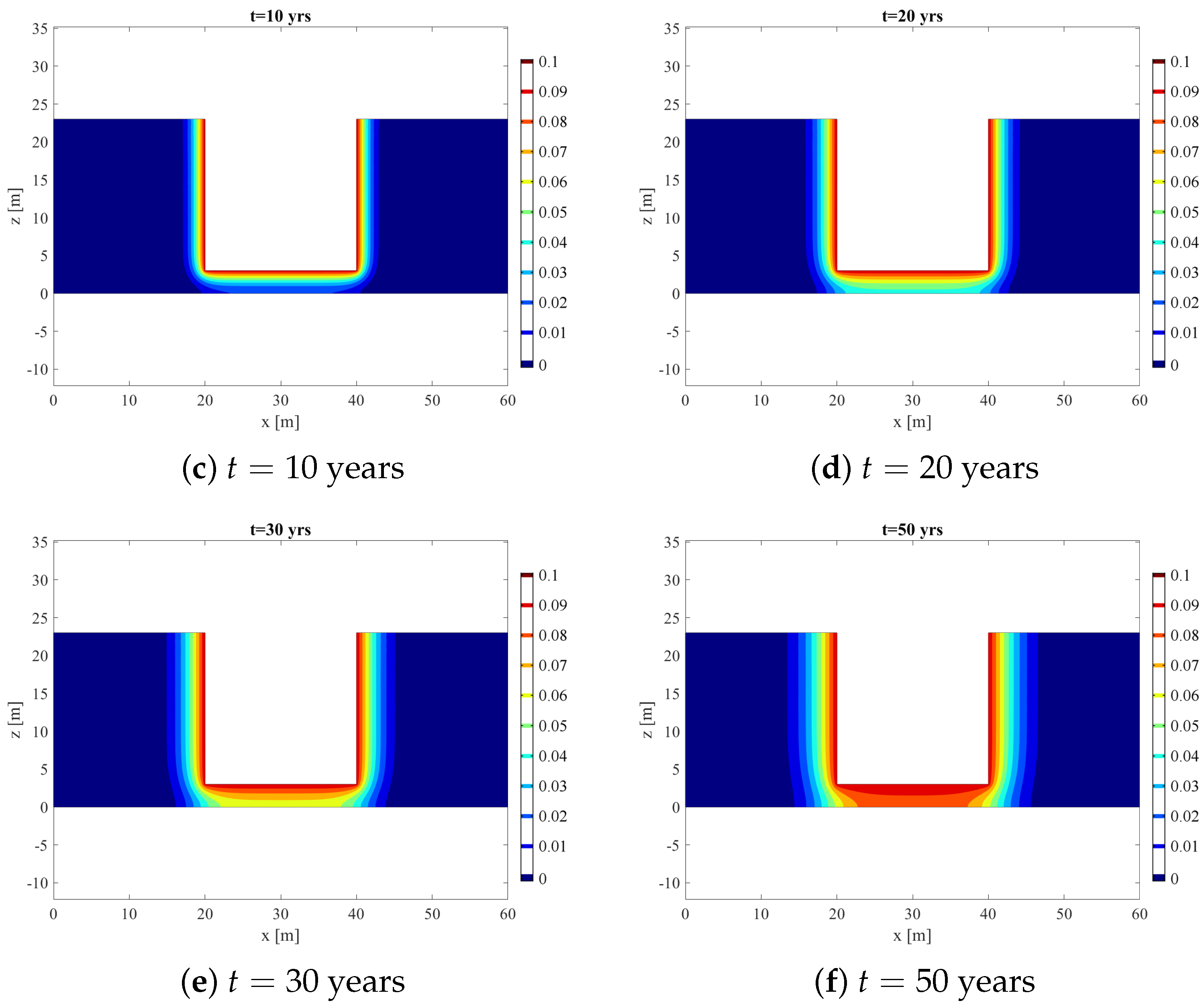
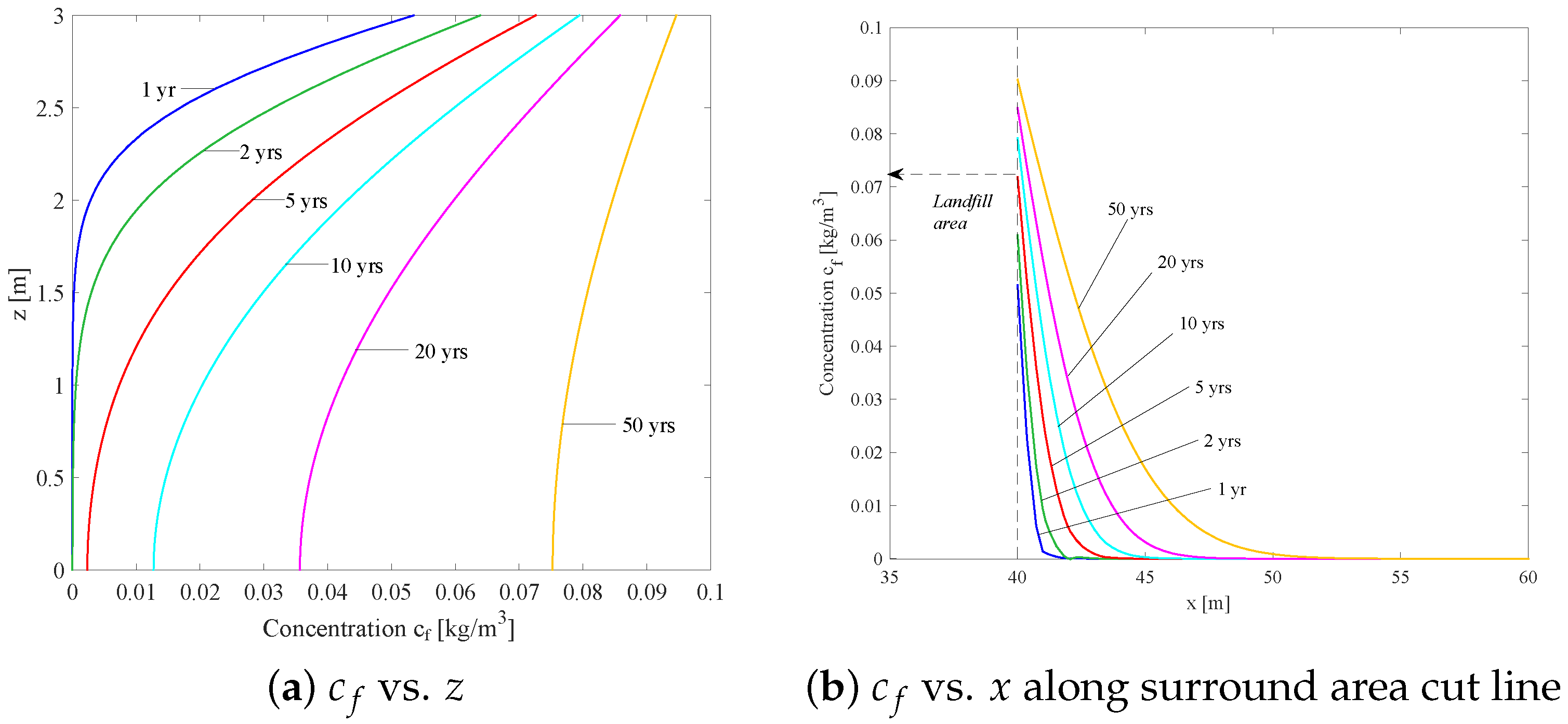
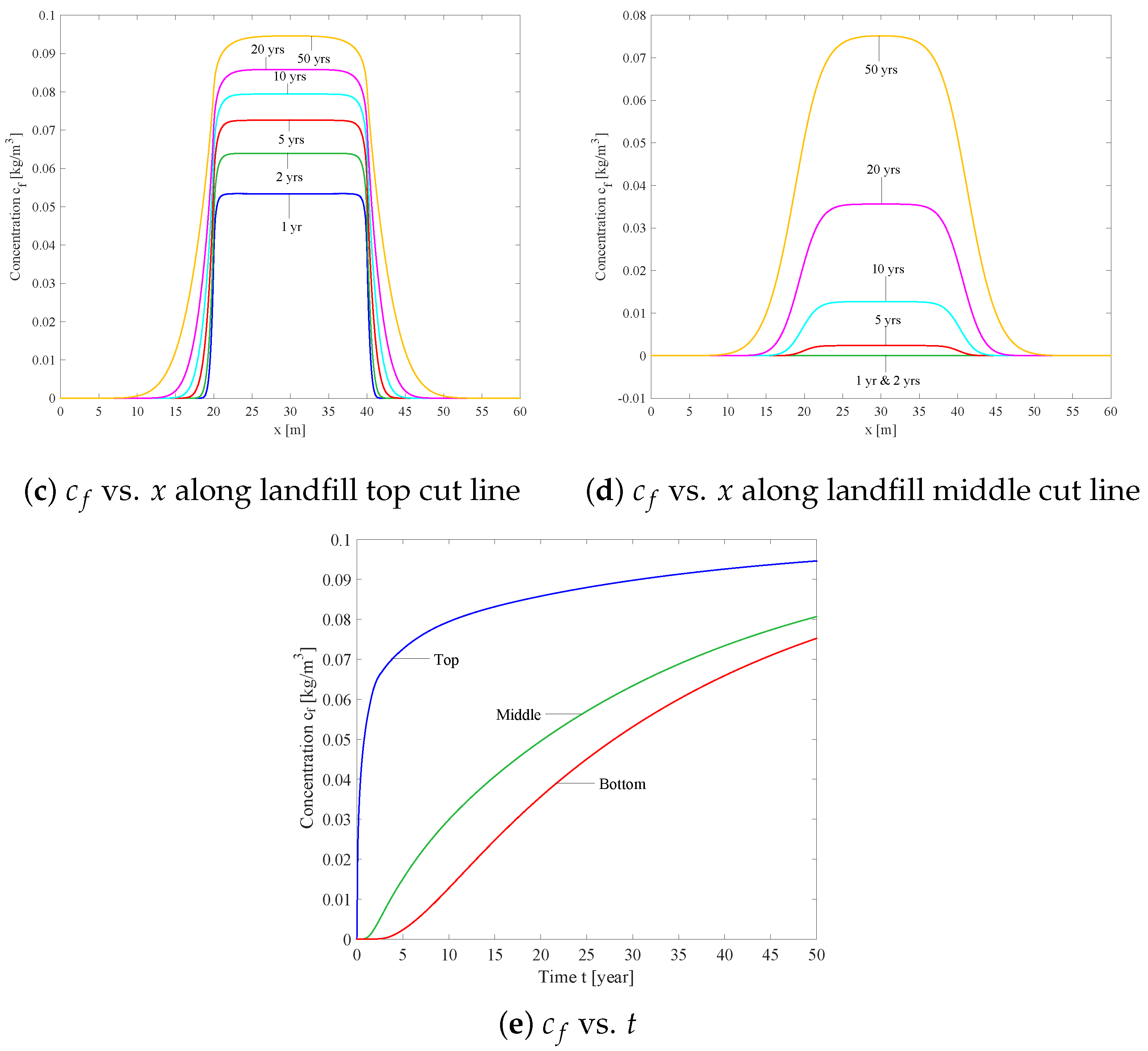
Lastly, the solute concentration contour diagrams from year 1 to year 50 are plotted in Figure 11. The pollution source is assumed to uniformly spread and exist in all three contact surfaces. All sub-figures are plotted with the same colour legend (0–0.1 kg/m${}^3$) to show the solute migration progress. Figure 12 shows the $c_f$ distribution at the center vertical cut line, as well as several horizontal cut lines and cut points. In general, solutes not only migrate in the vertical direction, but also spread horizontally into the surrounding area. However, it is obvious that solute spreads faster beneath the landfill than the surrounding area. Compared with Figure 12a,b, after 50 years, the solute concentration in the whole loaded area ($x=$ 20 m to $x=$ 40 m) is above 0.075 kg/m${}^3$, whereas in the surrounding area, this level of pollution only exists less than 1.5 m in the horizontal direction. This is mainly caused by the vertical transient flow, which is produced by soil consolidation. As shown in Figure 12c,d, at both $z=$ 3 m and $z=$ 5 m, solute spreads out and the contaminated zone expands over time. Specifically, at the end of 50 years, the contaminant spreads by around 10 m horizontally (Figure 12b–d).

4.2. Point-Source Pollution Study (2D)

In a realistic environment, pollution may occur at certain points instead of the whole contact surface. The whole computational domain is 300 m long and 23 m high, and the center-loaded area was assumed to be 100 m by 3 m. In order to analyse the pointed contaminant migration, three different types contaminant source were applied on the top surface of the loaded area (as shown in Figure 13). Instead of a uniform pollution source throughout the whole surface as introduced in the previous 2D model, the contaminant source was considered to only be applied in a small region in this point-source? pollution study.

In this case, a ramp load with loading rate of 200 kPa/year was applied to the entire top surface. After 2 years, the load stopped increasing and entered the post-loading stage with constant value of 400 kPa until the end of the model simulation. The pollution source distributions are summarised in

Table 4. Point-source pollution type.

Location	Pollution Region	Description
A	$x=$ 130 m to $x=$ 132 m	single pollution for 2 m
B	$x=$ 149 m to $x=$ 151 m	two 2 m pollution points
	and $x=$ 152 m to $x=$ 154 m	that are close to each other
C	$x=$ 170 m to $x=$ 174 m	single pollution for 4 m

.

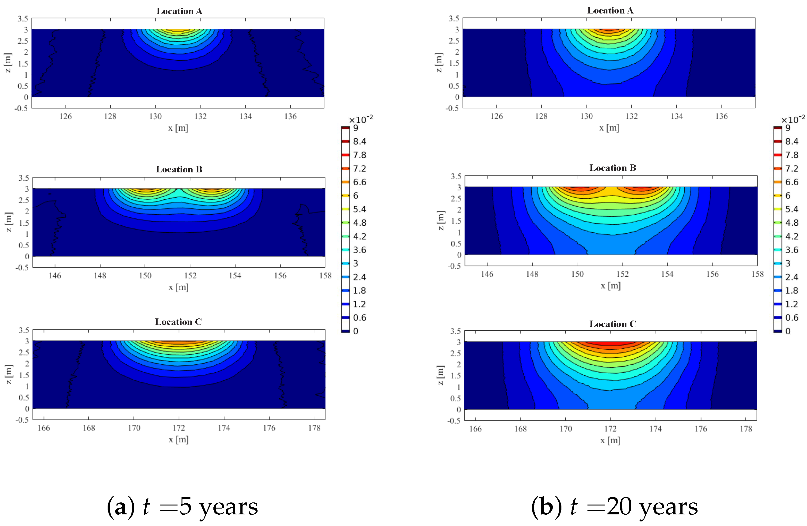
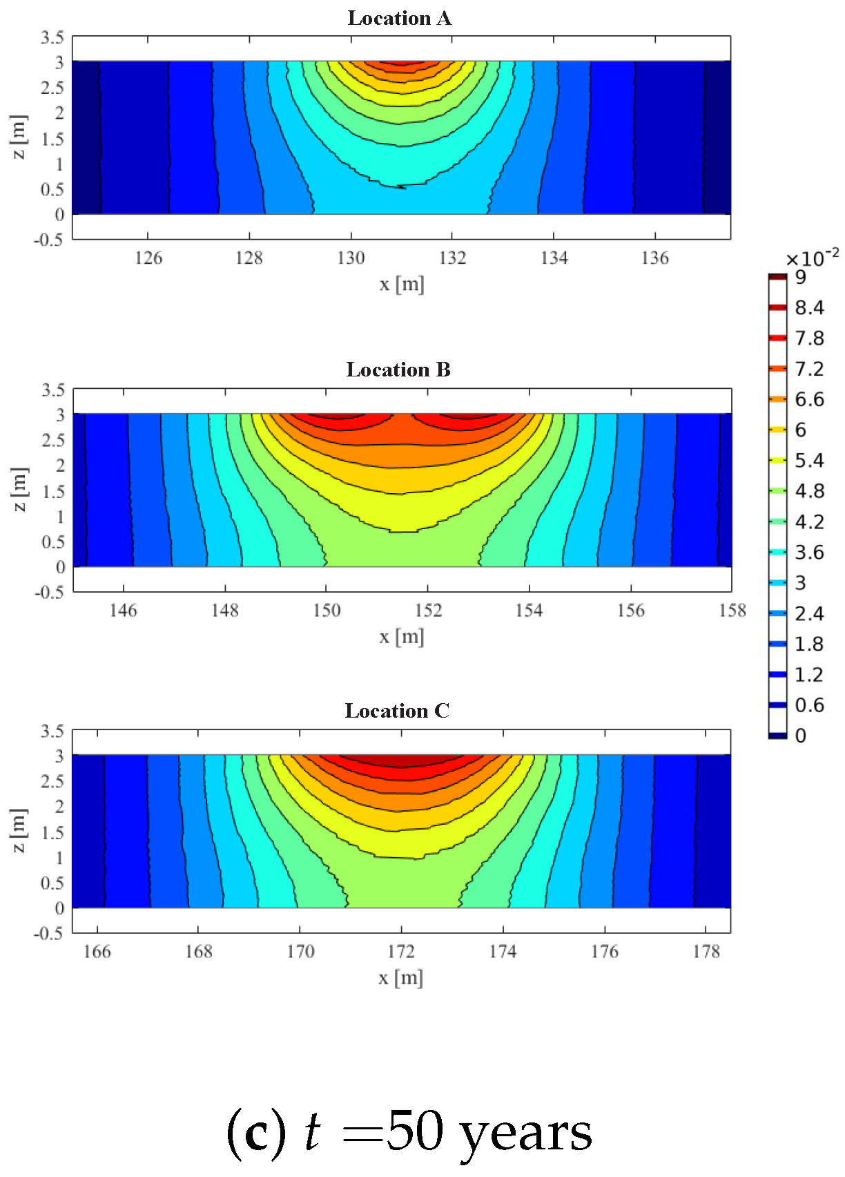
The contour diagrams focusing on the polluted area are shown in Figure 14a after 5 years, Figure 14b after 20 years and Figure 14c after 50 years. Sufficient space was ensured between each pollution source so that the pollution in each location would not influence the adjacent pollution point. The polluted area increased in all pollution locations with time as solute migrated in both directions. The polluted areas at Locations B and C generally had a similar size and were larger than those in Location A because the contaminant sources from Locations B and C were twice as wide as those in A.

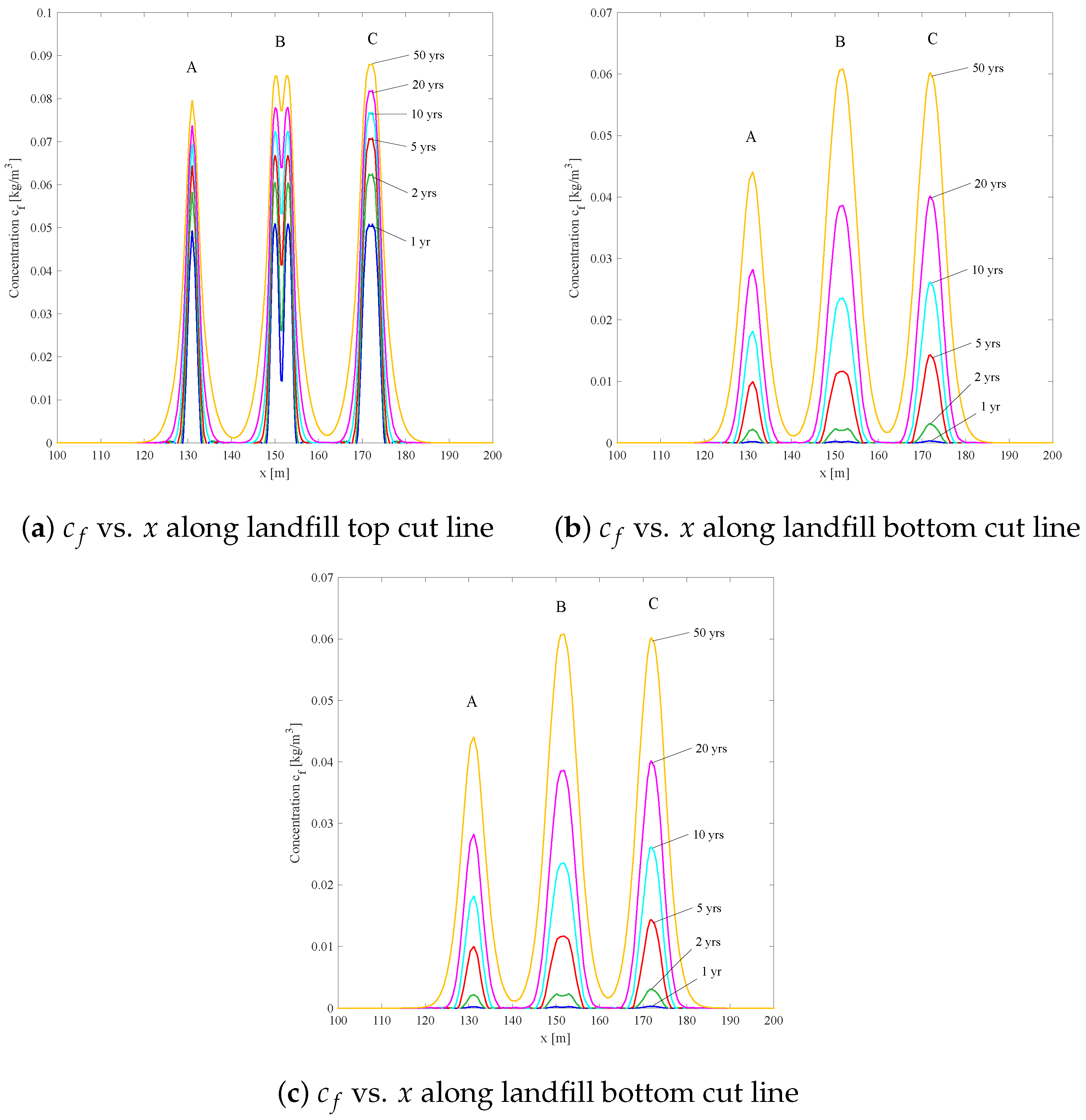
The solute concentration distribution along two horizontal cut lines shows the influences of point-source load near the pollution source. As shown in Figure 15a, at the pollution surface, although $c_f$ does not differ much at the beginning (at year 1, $c_f$ peaks at 0.05 kg/m${}^3$ in all locations), and this difference becomes more significant as the simulation continues. At the end of 50 years, peak $c_f$ are 0.08 kg/m${}^3$, 0.085 kg/m${}^3$ and 0.09 kg/m${}^3$ respectively. However, as the pollution source in Location C was twice as wide as that in Location A, the difference of 0.01 kg/m${}^3$ is not that obvious. As for Location B, where two 2 m contaminant sources are placed near each other, two peaks can be observed at all time steps. The peaks become less obvious as the simulation progresses. In terms of space, the two peaks no longer exist in the middle and bottom horizontal cut lines (Figure 15b,c). Near the bottom, $c_f$ at Locations B and C reaches 0.05 kg/m${}^3$, while Location A shows a lower contaminant concentration of 0.035 kg/m${}^3$. These trends cannot be shown in any 1D model, and the overall results highlight the impact of the size of the contaminant source onthe pollution level around the soil.

5. Conclusions

In this short communication, a 2D numerical model of consolidation-induced solute transport is proposed, with newly developed governing equations and boundary conditions. Due to the lack of field study and experimental studies, the present 2D model was validated by comparing with previous models [9,15]. With this 2D model, fully coupled soil consolidation and solute transport can be simulated in an unsaturated soil environment with time-dependent loading. The proposed 2D model is particularly useful in the following situations: i) when vertical (e.g., along the z-axis) load is applied on the site, and the pollution condition only matters in a particular horizontal direction; ii) when soil properties and pollutant propagation conditions are similar on both horizontal axes.

By conducting a 2D simulation with different pollution sizes and locations, the effects of a point-source contaminant were studied. The proposed 2D model was able to simulate the consolidation-induced solute transport in an anisotropic soil environment.

References

- Bear, J. Dynamics of Fluids in Porous Media; Elsevier Scientific Publishing Company: New York, NY, USA, 1972. [Google Scholar]
- Barry, D.A. Modelling contaminant transport in the subsurface: Theory and computer programs. In Modelling Chemical Transport in Soil: Natural and Applied Contaminants; Ghadiri, H., Rose, C.W., Eds.; Lewis Publishers: Boca Raton, FL, USA, 1992; pp. 105–144. [Google Scholar]
- Rolle, M.; Hochstetler, D.; Chiogna, G.; Kitanidis, P.K.; Grathwohl, P. Experimental investigation and pore-scale modeling interpretation of compound-specific transverse dispersion in porous media. Transp. Porous Media 2012, 93, 347–362. [Google Scholar] [CrossRef]
- Boso, F.; Bellin, A.; Dumbser, M. Numerical simulations of solute transport in highly heterogeneous formations: A comparison of alternative numerical schemes. Adv. Water Resour. 2013, 52, 178–189. [Google Scholar] [CrossRef]
- Wang, Q.; Zhan, H. On different numerical inverse Laplace methods for solute transport problems. Adv. Water Resour. 2015, 75, 80–92. [Google Scholar] [CrossRef]
- Alshawabkeh, A.; Rahbar, N.; Sheahan, T.C.; Tang, G. Volume change effects in solute transport in clay under consolidation. In Proceedings of the Advances in Geotechnical Engineering with Emphasis on Dams, Highway Materials, and Soil Improvement, Ibrid, Jordan, 12–15 July 2004; Volume 1, pp. 105–115. [Google Scholar]
- Potter, L.J.; Savvidou, C.; Gibson, R.E. Consolidation and Pollutant Transport Associated with Slurried Mineral Waste Disposal. In Proceedings of the 1st International Conference on Environmental Geotechnics, Edmonton, AB, Canada, 10–15 July 1994; pp. 525–530. [Google Scholar]
- Smith, D.W. One-dimensional contaminant transport through a deforming porous medium: Theory and a solution for a quasi-steady-state problem. Int. J. Numer. Anal. Methods Geomech. 2000, 24, 693–722. [Google Scholar] [CrossRef]
- Zhang, H.; Jeng, D.S.; Seymour, B.; Barry, D.A.; Li, L. Solute transport in partially-saturated deformable porous media: Application to a landfill clay liner. Adv. Water Resour. 2012, 40, 1–10. [Google Scholar] [CrossRef] [Green Version]
- Terzaghi, K. Erdbaumechanik auf Bodenphysikalischer Grundlage; Deuticke: Vienna, Austria, 1925. [Google Scholar]
- Wu, S.; Jeng, D.S. Numerical modeling of solute transport in deformable unsaturated layered soil. Water Sci. Eng. 2017, 10, 184–196. [Google Scholar] [CrossRef]
- Fox, P.; Berles, J. A piecewise-linear model for large strain consolidation. Int. J. Numer. Anal. Methods Geomech. 1997, 21, 453–475. [Google Scholar] [CrossRef]
- Fox, P. Coupled large strain consolidation and solute transport. I: Model development. J. Geotech. Geoenvironmental Eng. ASCE 2007, 133, 3–15. [Google Scholar] [CrossRef]
- Wu, S.; Jeng, D.S.; Seymour, B. Numerical Modelling of consolidation-induced solute transport in unsaturated soil with dynamic hydraulic conductivity and degree of saturation. Adv. Water Resour. 2020, 135, 103466. [Google Scholar] [CrossRef]
- Zhang, Z.H.; Fang, Y.F. A three-dimensional model coupled mechanical consolidation and contaminant transport. J. Residuals Sci. Technolocy 2016, 13, 121–133. [Google Scholar] [CrossRef] [PubMed] [Green Version]
- Wu, S. Numerical Simulation for Solute Transport in a Deformable Porous Medium. Ph.D. Thesis, Griffith University, Queensland, Australia, 2020. [Google Scholar]
- Biot, M.A. General theory of three-dimensional consolidation. J. Appl. Phys. 1941, 12, 155–164. [Google Scholar] [CrossRef]
- Fredlund, D.G.; Rahardjo, H. Soil Mechanics for Unsaturated Soils; Wiley: Hoboken, NJ, USA, 1993. [Google Scholar]
- Burnett, R.; Frind, E. An alternating direction Galerkin technique for simulation of groundwater contaminant transport in three dimensions, 2. Dimensionally effects. Water Resour. Res. 1987, 23, 695–705. [Google Scholar] [CrossRef]
- COMSOL. COMSOL Multiphysics, 3rd ed.; COMSOL: Shanghai, China, 2010. [Google Scholar]
Figure 1.
Sketch of 2D rectangular domain.
Figure 2.
Ramp load, , at the top of a soil layer in a landfill system.
Figure 3.
(a) Excesspore pressure ( (kPa)) and (b) vertical displacement (w (m)) at the top point (, ) vs. t and (c) solute concentration ( (kg/m)) at the bottom point (, ) from the 2D model with various soil domain lengths and the 1D model [9].
Figure 4.
The comparison of solute concentration distribution in the vertical direction for the present model (solid lines) and that of Zhang and Fang [15] (triangles and squares) with a constant loading. Note: results are present for simulation times of 5 years (red) and 10 years (black).
Figure 5.
Sketch of 2D landfill domain.
Figure 6.
Distribution of excess pore pressure ( (kPa)) from 1 year to 100 years.
Figure 7.
Excess pore pressure ( (kPa)) distribution along (a) center vertical cut line where 30 m; (b) top horizontal cut line where 3 m; and (c) (kPa) vs. t (years) at top cut point 30 m, 3 m, middle cut point 30 m, 1.5 m and bottom cut point 30 m, 0 m.
Figure 8.
Distributions of horizontal displacements (u (m)) from 1 year to 20 years.
Figure 9.
Distributions of vertical displacements (w (m)) from 1 year to 20 years.
Figure 10.
(a) Vertical displacement (w (m)) distribution along center vertical cut line ( 30 m); (b) w (m) vs. t (years) at top cut point 30 m, 3 m, middle cut point 30 m, 1.5 m and bottom cut point 30 m, 0 m; (c) horizontal displacement (u (m)) distribution along middle horizontal cut line at 1.5 m.
Figure 11.
Distribution of solute concentration ( (kg/m)) from 1 year to 50 years; note that all sub-figures share the same colour legend.
Figure 12.
Solute concentration ( (kg/m)) distribution along (a) center vertical cut line where 30 m; (b) horizontal cut line where 15 m; (c) top horizontal cut line where 3 m; (d) middle horizontal cut line where 1.5 m; and (e) (kg/m) vs. t (years) at top cut point 30 m, 3 m, middle cut point 30 m, 1.5 m and bottom cut point 30 m, 0 m.
Figure 13.
Sketch of point-source contaminant study case.
Figure 14.
Contour diagram of solute concentration ( (kg/m)) at Locations A, B and C after (a) 5 years, (b) 20 years and (c) 50 years.
Figure 15.
Solute concentration ( (kg/m)) distribution along horizontal cut lines (a) 3 m; (b) m and (c) m from 1 year to 50 years.