Validation of a Simplified Numerical Model for Predicting Solid–Liquid Phase Change with Natural Convection in Ansys CFX

Abstract

This paper presents a numerical model for simulating melting and solidification driven by natural convection, and validates it against a previous experiment. The experiment involved filling a rectangular aluminum enclosure with RT28HC Phase Change Material (PCM) to 95% of its capacity. To investigate the thermal behavior of the PCM during phase change, the enclosure underwent independent heating and cooling procedures. The simulation was conducted using ANSYS CFX^®, and the additional heat source (AHS) method was implemented in conjunction with the Boussinesq approximation to account for the latent heat during melting and solidification driven by natural convection. This allowed the calculation of temperature fields, the melted fraction, and fluid dynamics during phase change. The momentum equations were modified to include a source term that accounted for a gradual decrease in fluid velocity as the PCM transitions from solid to liquid. To account for density variation, an artificial specific heat curve was implemented based on the assumption that the product of density and specific heat remains constant during phase change. The proposed numerical model achieved good agreement with the experimental data, with an average root mean square error of 2.6% and 3.7% for temperature profiles during charging and discharging simulations, respectively. This model can be easily implemented in ANSYS CFX^® and accurately predicts charging and discharging kinetics, as well as stored/released energy, without any numerical convergence issues.

1. Introduction

Phase change materials (PMCs) play a crucial role in improving energy efficiency in various applications, from electronics to buildings [1]. PCMs are widely used for temperature regulation due to their energy storage capacity and isothermal behavior during phase change [2,3,4,5]. However, the low thermal conductivity of PCMs is a major drawback for their practical applications, resulting in slower heat transfer and lower heat storage and release rates [6,7]. The use of enclosures made of high thermal conductivity materials (macrocapsules), nanoparticles, and the incorporation of metallic fins within the PCM bulk have been recognized as effective techniques to enhance heat transfer rates and mitigate the limitations posed by the low thermal conductivity of PCMs [8,9]. According to the literature, different enclosure shapes have been found to have a significant influence on the thermal performance of thermal energy storage units [10,11].

In macro-encapsulated or free-form PCMs, heat transfer mechanisms during charging and discharging processes take place primarily through conduction and natural convection, the last being the most important process, especially in the melt region [12,13,14]. Numerical modeling of solid–liquid phase change problems is challenging due to their nonlinear nature at moving interfaces and the changes in the thermo-physical properties between phases. Despite the publication of numerous numerical studies over the past decade, there is still a lack of accurate numerical replication and validation of experiments.

In the literature, many studies have validated their phase change models using dimensionless parameters, but few have directly compared temperature profiles within the PCM. Numerical methods for modeling solid–liquid phase change can be classified into two categories: deforming-grid and fixed-grid methods [15,16,17,18]. While deforming-grid methods offer higher accuracy in localizing the phase interface, fixed-grid methods are computationally more efficient and employ well-established numerical techniques, making it possible to incorporate phase change modeling into commercial computational fluid dynamics software. There are several fixed-grid methods available for modeling phase change, including the enthalpy method, the heat capacity method, the temperature-transforming model, and the additional heat source method [19].

Early models based on the enthalpy formulation were investigated by Morgan [20], Gartling [21], and Voller [22,23,24]. These models formulated latent heat effects as a source term with linearization to improve numerical stability [25]. Brent et al. [26] used the enthalpy–porosity approach for modeling the convection–diffusion phase change, which achieved accurate results without requiring variable transformations. The enthalpy–porosity method has gained popularity within the research community and has been integrated into commercial CFD software packages, including ANSYS Fluent^®, which incorporates a built-in phase-change model. This model has been used to investigate the thermal performance of PCMs, as demonstrated in the work of Prieto et al. [27], where they assessed the fluid and heat transfer in PCM panels arranged both vertically and horizontally. Furthermore, the application of the enthalpy–porosity method has extended to practical scenarios. For instance, Wang et al. [28] investigated the impact of different fin geometries on enhancing the heat transfer performance of latent thermal energy storage systems. Additionally, Frazzica et al. [29] employed ANSYS Fluent^® to simulate a hybrid sensible–latent thermal energy storage system for supplying hot water on board ships.

Solving the solid–liquid phase change problem requires the use of the Navier–Stokes equations, adopting either the incompressible or compressible formulation. These equations are commonly solved using uncoupled solvers based on pressure discretization schemes such as SIMPLE, PISO, PRESTO!, and Body-Force-Weighted [30]. However, coupled solvers such as the one used in ANSYS CFX^®, which employs the Rhie–Chow interpolation method, may take longer to solve each iteration due to their complexity. Nevertheless, they tend to converge faster overall since they only need to converge the non-linear terms once, rather than repeatedly solving the linear terms separately. The ANSYS CFX^® software lacks a built-in phase-change model; thus, users are responsible for developing their own models to simulate phase-change phenomena. This lack of a dedicated model can potentially lead to unreliable results and necessitates additional time for modeling and calibration.

There are only a few studies in the literature that have used ANSYS CFX^® software to simulate phase change materials, such as those found in [31,32,33,34]. These studies primarily integrate source terms into the energy and momentum equations. One such method, the heat source method, involves incorporating latent heat in the energy equation via a time-varying term based on the melting fraction, and has been shown to yield good results in previous works [35,36,37,38,39,40]. To ensure that the velocity in the solid phase is small enough to be considered negligible, various solid velocity correction methods have been employed, including the switch-off method [20,21], variable viscosity [21,22,41,42,43,44,45], and the source term [18]. All methods require large numerical approximations to calculate the solid viscosity or scale the solid velocity, which can result in divergence problems. The source term method in the momentum equations is widely used by researchers working with commercial software.

The objective of this work is to develop a simple methodology using the additional source terms in the incompressible Navier–Stokes equations in ANSYS CFX^® to model the solid–liquid phase change with natural convection, including the validation of the numerical predictions against reliable experimental results. The numerical predictions will be validated using experimental data obtained from a previously developed laboratory setup designed to study heat transfer with solid–liquid phase changes within a rectangular enclosure [8,46,47]. The developed model holds promise in aiding engineers in the design and analysis of practical applications using ANSYS CFX^®, including PCM-based thermal energy storage systems, heat exchangers, and electronic applications [3,48,49,50].

2. PCM-Based Sample and Experimental Method

The thermal energy storage (TES) unit under study (as shown in Figure 1a) is a 300 × 300 × 30 aluminum enclosure with 2 mm thick walls and an aspect ratio (A = W/H) of 11.385. It is filled with 95% PCM (RT28HC). The experiments reported by Soares et al. [8,46,47] were used to validate the numerical simulations of the TES unit. In the laboratory setup, the PCM-based sample was fixed in a vertical position and thermally insulated on its smaller border faces, so that only the right and left larger surfaces were thermally active. On the left side of the enclosure, a heating module holding a 64 W electrical resistance (the hot plate) was tightly fixed to perform charging experiments. During the charging process, as shown in Figure 1a, a thermal insulation board was placed on the right side of the sample to ensure adiabatic conditions.

For discharging, a cooling module holding a heat exchanger fed by a thermally regulated water flow (the cold plate) was placed tightly on the right side of the PCM-based sample, and a thermal insulation board was placed on the left side of the sample to ensure adiabatic conditions.

Before each charging experiment, the TES unit was pre-cooled to 13 °C and the hot plate was pre-heated to 55 °C. The charging experiment was stopped when the temperatures measured by all sensors within the PCM reached 55 °C. The discharging experiment was initiated after the charging process and was stopped when the PCM bulk temperature reached 14 °C, as specified by the thermostat of the cold water bath. Twenty-one K-type thermocouples were distributed on the left and right surfaces of the test sample to measure the surfaces’ transient evolution (Figure 1b). T_H (t) and T_C (t) represent the average temperatures measured on the hot and cold plates, respectively. These temperature profiles were used as time-varying boundary conditions in the numerical simulations. Five K-type thermocouples were placed on the mid-plane of the TES unit to measure the temperature distribution within the PCM domain during the charging and discharging processes (Figure 1c).

The data acquisition system consisted of several Pico^® TC-08 thermocouple data loggers (with an accuracy of ±0.2%, corresponding to ±0.5 °C) connected to a computer and controlled by the PicoLog^® data acquisition program. Data from all sensors were collected and stored at 30-s intervals. Further details about the experimental setup, instrumentation, and procedure can be found in references [8,46,47].

3. Material Properties

The accurate modeling of melting and solidification driven by natural convection in PCM RT28HC requires a comprehensive understanding of its thermo-physical properties. Data provided by manufacturers is often incomplete or uncertain, leading to potential errors in simulations. The main thermo-physical properties of the RT28HC were previously determined [8] and compared with the manufacturer’s specifications, as presented in

Table 1. Main thermo-physical properties of the PCM-based samples used in the experiments.

	Macroencapsulated RT28HC PCM
	Measured Values [8]	Data from Manufacturer [52]
Melting peak temperature, Tm [°C]	27.55 ± 0.19	28
Solidification peak temperature, Ts [°C]	25.71 ± 0.10	27
Heat storage capacity [kJ/kg]		250 ± 7.5% [21–36 °C]
Latent heat [kJ/kg]
Melting, Lm	258.1 ± 5.1 [20–30 °C]	250
Solidification, Ls	251.9 ± 6.7 [20–27 °C]	250
Specific heat [J/kg⸳°C]
Solid, cp,s	1652 ± 105 [0–20 °C]	2000
Liquid, cp,l	2021 ± 120 [35–45 °C]	2000
Thermal conductivity [W/(m⸳°C)]
Solid, ks	≈0.34 ± 0.00	0.2
Liquid, kl	≈0.19 ± 0.00	0.2
Volumetric mass density, ρ [kg/m3]
Solid, ρs	-	880
Liquid, ρl	-	770
Thermal expansion, β [K−1]	-	0.001
Dynamic viscosity, µ [Pa.s]	-	3.1 × 10−3

. The data sheet of the manufacturer states that the heat storage capacity of the PCM was considered as a combination of latent and sensible heat in a temperature range of 21 to 36 °C, and the density of the PCM was measured at 15 and 40 °C for solid and liquid phases, respectively. The melting area was in the range of 27–29 °C with the main peak at 28 °C, while the congealing area was in the range of 29–27 °C with the main peak at 27 °C. As noted by Dutil et al. [51], it is imperative to have a clear understanding of the PCM’s overall thermal behavior to avoid intrinsic inaccuracies in simulations.

The measurement of thermal conductivity was carried out using the transient plane source (TPS) method, which was performed on Hot Disk TPS 2500 S equipment. The measurements were conducted in the temperature range of 0 to 50 °C, with a temperature interval of 5 °C [8]. The melting and solidification temperatures, as well as the latent heat of fusion and solidification, were determined through modulated differential scanning calorimetry (MDSC) using a Q100 model equipment from TA Instruments [8]. The specific heat of both the solid and liquid phases were also obtained through the same MDSC measurements.

The melting and solidification peak temperatures determined through experiments were lower than the values provided by the manufacturer. The difference between the melting temperature (T_m) and the solidification temperature (T_s) is referred to as the hysteresis temperature difference (∆T_hyst) and must be considered in the simulations. In the present case, the experimental value for ∆T_hyst is ≈ 2 °C. The measured values for the latent heat of fusion (L_m), specific heat in the liquid state (c_p,l), and thermal conductivity in the liquid state (k_l) were consistent with the manufacturer’s data sheet. However, the values for the solid-state properties (c_p,s and k_s) were slightly lower than those provided by the manufacturer. The manufacturer’s data sheet provides constant values for both solid and liquid phases. The weight of the PCM was determined by weighing the TES units, both empty and filled.

The thermal expansion coefficient of the PCM is given by:

$${\left.\beta =-\frac{1}{{\rho }_{ref}}\frac{{\partial }_{{\rho }_l}}{\partial T}\right|}_{T_m}$$

(1)

where ${\rho }_{ref}$ is taken as the mean density between the solid and liquid state and ${\rho }_l$ is the density in the liquid region.

The thermo-physical properties of the aluminum enclosure used to heat or cool down the PCM, as well as the properties of the air cavity above the PCM, are presented in

Table 2. Thermo-physical properties of the enclosure and air.

	Aluminium [53]	Air at 25 °C
Density, ρ [kg/m3]	2707	1.185
Specific heat, cp [J/(kg⸳°C)]	896	1004.4
Thermal conductivity, k [W/(m⸳°C)]	204	0.0261
Dynamic viscosity, µ [Pa⸳s]	-	1.83 × 10−5
Thermal expansion, β [K−1]	-	0.003356

. The air domain was set to constant temperature at 25 °C for the purpose of the simulation.

4. Numerical Model

The numerical model developed to reproduce experiments was comprehensive considering several simplifications and assumptions. The model was built using the commercial computational fluid dynamics ANSYS CFX^®. The Navier–Stokes equations for energy, momentum, and continuity were solved using a fixed-grid finite volume method, with elements based on cell vertex. Source terms were added to the energy equation to simulate the latent heat during phase change and to the momentum equations to ensure that the material velocity was zero during the solid state. The density difference in the liquid phase due to the non-uniform temperature field creates buoyancy and associated liquid phase movements. Therefore, the Navier–Stokes equations had to be solved to accurately model these effects. Vogel and Thess [54] compared the volume of fluid method that considers variable properties with a simplified model that uses the Boussinesq approximation and constant properties. They found that the simplified model is not capable of reproducing the melting process with enough detail, but it is still sufficiently accurate for the design of latent thermal energy storage systems. In light of this, the present model incorporates the Boussinesq approximation, which assumes constant density and disregards volume expansion during the phase change. Additionally, the following assumptions were made in the numerical model:

• Heat transfer within the PCM and air domain occurs through conduction and convection;
• The flow of liquid phase in the PCM is considered to be incompressible;
• Both the air and PCM flows are assumed to be laminar, which is supported by a Rayleigh number below 10⁸, indicating a buoyancy-induced laminar flow [55];
• Viscous dissipation is neglected in the liquid phase of the PCM;
• The hysteresis of melting and solidification is accounted for by considering a ∆T_hyst value in the problem formulation, considering the differences between L_m and L_s, and assuming the different heating and cooling responses of the PCM;
• The thermo-physical properties of the materials are assumed to be independent of temperature, except for the PCM-based materials, where the specific heat capacity (c_p) and thermal conductivity (k) are considered to differ between the solid and liquid phases, and thermal conductivity is assumed to vary with temperature;
• The influence of PCM expansion and contraction during phase change is not considered, resulting in a constant density assumption, although this effect is implicitly considered in the temperature-dependent artificial curve for specific heat capacity;
• All materials are assumed to be homogeneous and isotropic.

The experimental setup was developed to enable the future validation of a simplified two-dimensional numerical model. To expedite model calibration and analysis, the inclusion of a 3D configuration was deemed unnecessary for this case study. By adopting this approach, a substantial reduction in computational time was achieved while still accurately predicting the charging and discharging kinetics, as well as the stored and released energy. To overcome the limitation of CFX not allowing 2D simulations, the third dimension was treated as equivalent to the height and width of the control volume. As a result, only one layer of elements was employed in the direction of thickness.

4.1. Mathematical Model

The numerical model for the phase change thermal energy storage system used the unsteady Navier–Stokes equations, which are standard for modeling incompressible flows. These equations are represented by the continuity equation (Equation (2)), the momentum equation (Equation (3)), and the energy equation (Equation (5)).

The continuity equation is:

$$\nabla .U=0$$

(2)

The momentum conservation equation is:

$$\rho \frac{\partial U}{\partial t}+\rho \nabla .\left(U\otimes U\right)=-\nabla p+\nabla .\tau +S_b+S_M$$

(3)

where ρ [kg/m³] is the density, which is constant for an incompressible flow; t [s] is the time; U [m/s] is the velocity of fluid; p [Pa] is the pressure; S_b and S_M are source terms [kg/(m²⸳s²)]; and τ is the stress tensor, which is related to the strain rate by

$$\tau =\mu \left(\nabla U+{\left(\nabla U\right)}^T-\frac{2}{3}\delta \nabla \cdot U\right)$$

(4)

The thermal energy equation, suitable for low-speed flows and where the variable-density effects are negligible, is written as:

$$\rho \frac{\partial \left(c_{p}T\right)}{\partial t}+\rho \nabla .\left(Uh\right)=-\nabla \cdot \left(k\nabla T\right)+\tau :\nabla U+S_f$$

(5)

where c_p [J/(kg⸳°C)] is the specific heat at constant pressure, T [°C] is the temperature, k [W/(m⸳°C)] the thermal conductivity, and S_f is the additional heat source term [W/m³]. Since the viscous dissipation is neglected,

$$\tau :\nabla U=0$$

(6)

For the buoyancy calculation, a source term is added to the momentum equation as follows:

$$S_b=(\rho -{\rho }_{ref})g$$

(7)

where g [m/s²] is the gravitational acceleration. Because the Boussinesq approximation is being used, a constant reference density ρ_ref is used in all terms except in the buoyancy source term. The buoyancy source term is modeled as:

$$(\rho -{\rho }_{ref})=-{\rho }_{ref}\beta (T-T_{ref})\hspace{1em}\hspace{1em}\hspace{1em}\hspace{1em}\hspace{1em}\hspace{1em}\beta (T-T_{ref})<<1.0$$

(8)

The thermal expansion is given by Equation (1), and T_ref is the buoyancy reference temperature which was equal to the average temperature of the PCM domain.

4.1.1. Additional Heat Source Method

The additional heat source term, S(f), was included to account for the local rate of latent heat being stored or released during the phase change, which is caused by the variation in the PCM’s melted fraction, f(T). This term is expressed as:

$$S\left(f\right)=-\rho L_m\frac{\partial f}{\partial T}\frac{\partial T}{\partial t}$$

(9)

As noted by Heim [56], the value of this term is negative when the PCM is receiving energy and is positive when the material is releasing the stored heat. This term is equal to zero when the PCM temperature is outside of its phase-change temperature range, i.e., when T ≤ T_1m and T ≥ T_2m (for charging), and when T ≤ T_1s and T ≥ T_2s (for discharging). The PCM’s melted fraction is obtained at each time step as a function of the computed temperature T (Figure 2), as follows:

$$f\left(T\right)=\left\{\begin{array}{l}0\hspace{1em}\hspace{1em}\hspace{1em}\hspace{1em}\hspace{1em}\hspace{1em}\hspace{1em},T\le T_{1K};\\ f_K\left(\frac{T-T_{1K}}{\mathsf{\Delta }{T}_{1K}}\right)\hspace{1em}\hspace{1em}\hspace{1em}\hspace{1em},T_{1K}<T<T_K;\\ f_K+\left(1-f_K\right) \left(\frac{T-T_K}{\mathsf{\Delta }{T}_{2K}}\right)\hspace{1em},T_K<T<T_{2K};\\ 1\hspace{1em}\hspace{1em}\hspace{1em}\hspace{1em}\hspace{1em}\hspace{1em}\hspace{1em},T\ge T_{2K};\end{array}\right.K=\mathrm{m},\mathrm{s}$$

(10)

$$f_K=\frac{\mathsf{\Delta }{T}_{1K}}{\mathsf{\Delta }{T}_K};\hspace{1em}K=\mathrm{m},\mathrm{s}$$

(11)

Equation (10) was used to model the charging and discharging processes using the AHS method. When defining the variables f_m and f_s through Equation (11), the resulting melted fraction f(T) exhibits linear variation in the mushy region. However, in cases where the PCM has significantly different values of f_m and f_s, the modeler may wish to specify peak values of the melted fraction in these regions using two-step linear formulations, as shown schematically in Figure 2.

For reasons of simplification, f_m = f_s = 0.5 was considered in the present study resulting in a one-step linear variation of f(T). However, alternative approaches in the literature [57,58] employ sine or Gaussian functions to predict the evolution of the melted fraction of the PCM.

In order to ensure numerical convergence, a linearization or source coefficient must be established for the nonlinear source [59]. This can be achieved by using the following expression to set the source coefficient in CFX:

$$\frac{\partial S\left(T\right)}{\partial T}=-a\cdot \frac{\rho L}{\mathsf{\Delta }t},\mathrm{where}\left\{\begin{array}{c}a=0 ,T_{1m}\ge T\ge T_{2m}\\ a=\frac{1}{\mathsf{\Delta }{T}_m} ,T_{1m}<T<T_{2m}\end{array}\right.$$

(12)

where Δt [s] is the time step. For stability reasons, the source coefficient must have negative value.

4.1.2. Momentum Source Method

To address the phase transition from liquid to solid, CFX provides two methods for solving the Navier–Stokes equation: using momentum source terms or increasing the effective viscosity as a function of temperature. However, the latter method can result in high numerical instabilities and temperature fluctuations. Alternatively, CFX allows for direct specification of the momentum source, S_M, by defining a force per unit volume in a specific direction.

The momentum sources are set for the three directional components by:

$$\begin{gathered} S_{M,x}=-C\left(f\right)\left(U_x-U_{spec}\right) \\ {S}_{M,y}=-C\left(f\right)\left(U_y-U_{spec}\right) \\ {S}_{M,z}=-C\left(f\right)\left(U_z-U_{spec}\right) \end{gathered}$$

(13)

The function C(f) depends on the liquid phase fraction, which is described in Equation (10). The velocity vector is then multiplied by this function, where U_spec [m/s] represents the specified velocity in the solid phase, which is set to 0 m/s. When the function takes on large values in the solid phase, it forces the velocities to converge towards zero values within the linear system [26]. The function C(f) (Equation (14)) is used to make the momentum equations mimic the Carman–Kozeny equations [60] for flow in porous media. Carman–Zozeny deals with fluid flow through porous media, but in this study, the conventional concept of porosity was replaced by a function f(T). This represents a novel approach, diverging from the methods proposed and employed in previous research works, including the work by Brent et al. [26].

$$C(f)=C\frac{{\left(1-f\left(T\right)\right)}^2}{f(T{)}^3+0.001}$$

(14)

The constant C [kg/(m³ s)] represents the mushy region constant and plays a significant role in the kinetic processes within the mushy region. It reflects the morphology of the melting front, which affects the phase transition from liquid to solid. To avoid division by zero, a small number of 0.001 is introduced in Equation (14). Shmueli et al. [30] have studied the influence of the constant C. In the literature, C values of 10⁵ (e.g., [61,62,63]) or 10⁶ (e.g., [54,64]) are commonly used. In a study conducted by Fadl et al. [65], it was concluded that smaller values (<10⁵) lead to unrealistic predictions of the melt front development, while higher values (10⁶) result in delayed melting predictions for the PCM. Ebrahimi et al. [66] found that the solid–liquid interphase morphology and the rate of phase change are highly sensitive to the C value, depending on the thickness of the mushy zone and velocity fields. After conducting exploratory numerical simulations, and for this specific PCM, a value of 10⁵ was chosen for C in this study to avoid numerical divergence issues and unrealistic predictions.

To enhance numerical convergence, the momentum source coefficient in ANSYS CFX^® setup was set to be—C(f). Both the momentum source, S_M, and C(f) were incorporated into the Rhie–Chow redistribution algorithm and coefficient, respectively, to ensure that the mass flow aligns with the specified velocity.

4.1.3. Modeling of Material Properties

The material properties of the PCM were modeled using the Boussinesq approximation, which assumes that the density is constant in all terms except for the linearized buoyancy term in the momentum equation. The selected reference density was that of the solid state, although the melting process is governed by natural convection in the liquid state. Consequently, the amount of sensible heat in the liquid state could be overestimated. To address this issue, the specific heat was adjusted in the liquid state based on energy balances.

$$c_{p,l.eq}=\frac{{\rho }_{ref}{c}_{p,s}}{{\rho }_l}$$

(15)

where c_p,l.eq [kJ/(kg⸳°C)] is the equivalent specific heat at the onset of the liquid state. Additionally, as the density decreases with temperature in the liquid state, as described in Equation (8), the specific heat during the liquid state, c_p,l (T) [kJ/(kg⸳°C)] can be calculated as follows:

$$c_{p,l}(T)=\frac{1}{\beta \left(T-T_{2m}\right)+1}{c}_{p,l,eq}$$

(16)

The specific heat capacity during the phase change depends on the fraction that has melted:

$$c_p\left(T\right)=f\cdot c_{p,l.eq}+(1-f)c_{p,s}$$

(17)

The variation in volumetric heat capacity (VHC) with temperature is presented in Figure 3a. The thermal conductivity was implemented in the CFX simulations using the measured values shown in Figure 3b [8], and it was assumed to have a linear variation during the phase change. Although the material datasheet provided a constant value for dynamic viscosity, which is a temperature-dependent property, the dynamic viscosity, µ [kg/(m.s)], of the PCM was calculated using the following function:

$$\mu =\mathit{exp}\left(A+\frac{B}{T}\right)$$

(18)

where the constant coefficients were established as A = −3.8 and B = 1790.

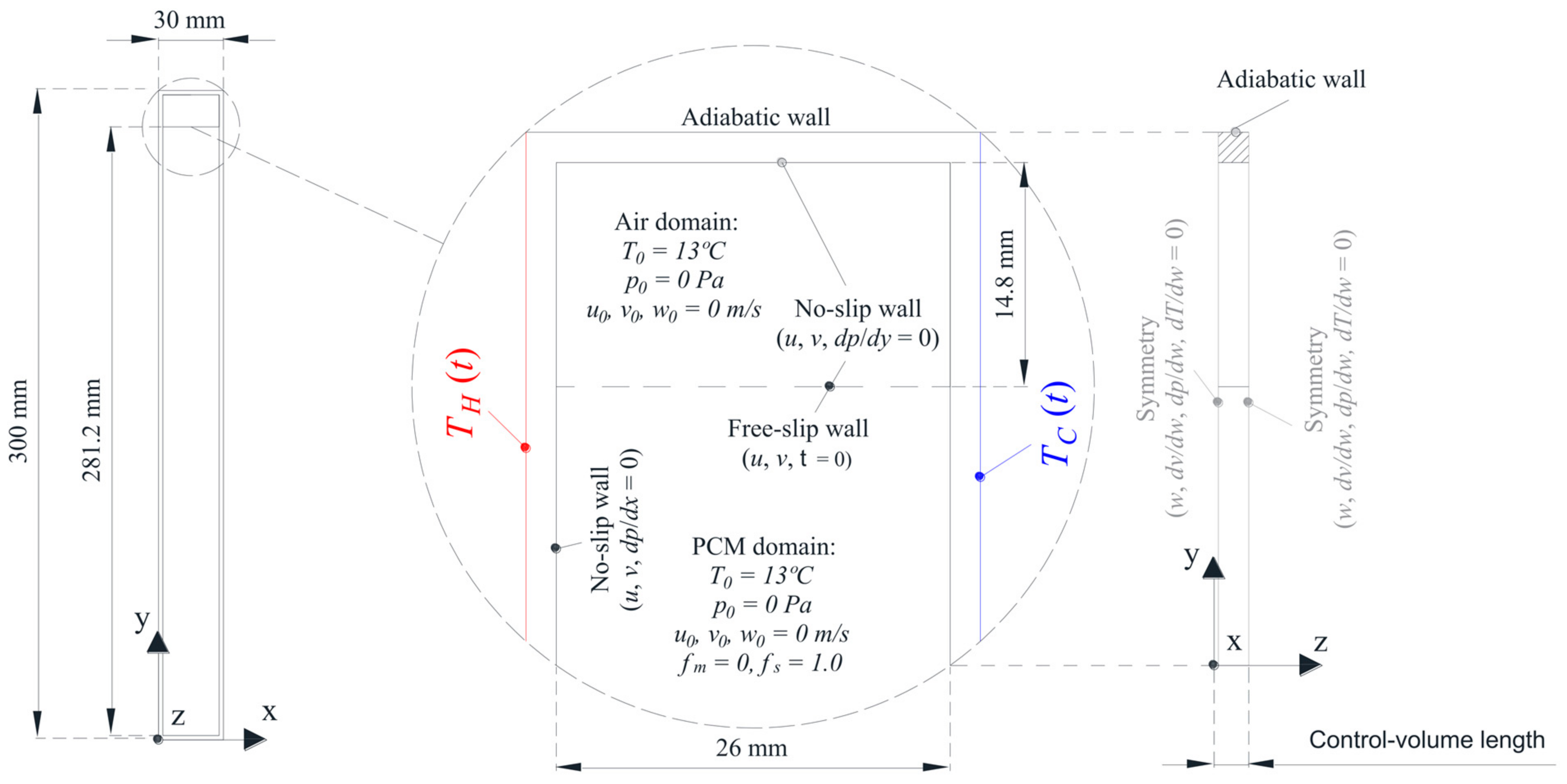
4.2. Initial and Boundary Conditions

The boundary conditions were imposed on the vertical surfaces on the left and right of the rectangular enclosure and were set to the values of T_H (t) and T_C (t) recorded during the charging and discharging experiments on the PCM-based sample, as illustrated in Figure 4. The top and bottom boundaries were assumed to be adiabatic. As previously mentioned, CFX does not support the use of 2D models, so a depth with the same size as the control volume height and width was considered. At the front and back surfaces of the enclosure, symmetry conditions were imposed. The inner walls of the enclosure were set with zero fluid velocity (no-slip wall condition), resulting in no relative movement between the fluid and the wall. Since the numerical model simulates the interface between air and PCM using a fixed grid and incompressible flow, the interface between both fluids was established as follows: zero velocity at the interface between air and PCM on the air domain side and free-slip wall on the PCM side (Figure 4), allowing the PCM fluid to adopt the velocity of the interface. To enable CFX-Pre to recognize the two different fluid materials, the beta features must be enabled, and the constant domain physics needs to be disabled [31].

The Initial conditions were set to be equal to those Imposed In the experiments, as described in Section 2. At the beginning of the charging simulations for the TES unit, the numerical domain was assumed to be at a uniform temperature of ${\left(T_i\right)}_{t=0}={\left(T_{\mathrm{PCM}}\right)}_{t=0}=13.07 °\mathrm{C}$. During the charging simulation, both the PCM and air domains were initialized with zero velocity (u₀, v₀, w₀) and zero pressure (p₀). The charging simulation concludes when the temperature of the PCM, T_PCM, reaches 55 °C. In contrast, the discharging simulation ends when T_PCM reaches 14 °C. The discharging simulation uses the temperature and velocity fields achieved at the end of the charging simulation as its initial conditions.

At each time step, the total PCM melted fraction, F, is calculated during charging and discharging, according to:

$$F=\frac{{\sum }_i{\sum }_j{\sum }_k{f}_{i,j,k}}{N_{CV}}$$

(19)

The local melted fraction of the PCM, f_i,j,k, is calculated at each control volume (I,j,k) in the simulation considering the total number of control volumes (N_CV). To assess the accuracy of the simulation, the root mean square error (RMSE) measures the standard deviation of the errors in the temperature prediction as follows:

$$\mathrm{R}\mathrm{M}\mathrm{S}\mathrm{E}\left(\%\right)=\frac{\sqrt{\frac{{\sum _{i=1}^n\left(T_{\mathrm{E}, \mathrm{i}}-T_{N,i}\right)}^2}{n}}}{R}\times 100$$

(20)

where T_{E, I} and T_{N, I} are the experimental and numerical temperature at T₁ to T₅ for a given time step I, n the number of data points, and R represents the range of temperature between initial conditions and final results. Additionally, the time required for complete melting (t_m,num) and solidification (t_s,num) of the PCM in the numerical domain during the charging and discharging simulations, respectively, are computed. The derivate of temperature is used to identify the transition times between the melting and solidification plateaus, which are often reported as “extended plateaus” in the literature.

The total energy stored or released by the PCM-based TES units during charging and discharging, E_m,1 and E_s,1, respectively, can be calculated by integrating the instantaneous heat rate across the aluminum–PCM interface over time. To determine the effectiveness of the simulated charging cycle of the PCM, the value of E_m,1 will be compared to the value of the stored energy during a complete simulated charging cycle of the PCM, E_m,2. E_m,2 is calculated by using the distribution of temperature in the PCM domain at the beginning and at the end of each charging simulation, as given by Equation (21). In Equation (21), the volume of each control volume occupied by the PCM is represented by V. The final and initial temperatures reached by the PCM at each control volume (I,j,k) are represented by T_f and T_i, respectively. The same procedure is considered for the discharging simulations, where E_s,1 is compared to E_s,2.

$$E_{m,2}=\sum _i\sum _j\sum _k{\rho }_{i.j.k}{ V}_{i.j.k}\left[c_{ps}\left(T_{1,m}-T_i\right)+\left(\frac{c_{ps}+c_{pl}}{2}\right)\left(T_{2,m}-T_{1,m}\right)+L_m+c_{pl}\left(T_{\mathrm{f}}-T_{2m}\right)\right]$$

(21)

4.3. Numerical Procedure

The analytical heat source (AHS) method was implemented using ANSYS CFX^®, which is a control volume-based code that uses cell vertex finite volume discretization with a high-resolution advection scheme. The rectangular geometry was discretized using ANSYS meshing, resulting in a structured quadrilateral mesh. Stability, convergence, and mesh independence were evaluated to ensure that the solution did not change significantly with further refinements of the spatial discretization. Mesh independence was achieved when the variation of the total stored (E_m,1 and E_m,2) or released energy (E_s,1 and E_s,2) between two consecutively refined meshes (at a mesh refinement ratio of 1.5) was lower than 2% for the charging and discharging simulations. The optimal control volume size of 0.5 × 0.5 × 0.5 mm³ was determined through a mesh dependency study, leading to a mesh with 36000 elements and 76064 nodes.

An adaptive time-step approach was employed with the following parameters: (i) a minimum and maximum time step of 2 s and 10 s, respectively; (ii) an initial time step of 0.001 s; and (iii) convergence was based on the Courant number of 0.5, considering the mesh size, time step size, and fluid velocity predictions. The simulation was considered converged when the root mean square (RMS) residuals met a target of 10⁻⁶, with a maximum of 100 iterations allowed per time step. Additionally, global imbalances were monitored and maintained below 1%. The simulations were performed using an Intel Core i9-7900x CPU@3.30 GHz with 32 GB RAM–20 logical processors used during calculation.

5. Results and Discussion

After a complete analysis and considering the assumptions mentioned above, the computational fluid dynamics (CFD) model was validated. A comparison between the measured temperature profiles at five different points and the corresponding numerical results is shown Figure 5a,c for the charging and discharging simulations, respectively. The RMSE, the time required for complete melting (t_m,num) and solidification (t_s,num), and the energy storage and release were calculated using both measured and numerical data and they are presented in

Table 3. Computed variables during charging and discharging vs. experimental results.

Charging						Discharging
Em,1 (kJ)	Em,2 (kJ)	Point	tm,numerical (s)	tm,experimental (s)	RMSE (%)	Es,1 (kJ)	Es,2 (kJ)	Point	ts,numerical (s)	ts,experimental (s)	RMSE (%)
702.9	702.9	T1	4336	4380	2.5	625.8	625.8	T1	29,304	14,040	5.3
		T2	6316	5820	2.7			T2	29,264	21,270	3.9
		T3	7528	7230	2.3			T3	29,246	23,700	3.5
		T4	8516	8550	3.6			T4	29,236	26,430	3.1
		T5	9500	10,350	9.8			T5	29,238	26,460	3.0

. During the charging process, there was good agreement between the measured and numerical temperature profiles, with RMSE values ranging from 2.5% to 3.6% at points T₁ to T₄, respectively. However, for T₅, a RMSE value of 9.8% was obtained. This point, located near the enclosure’s bottom surface, showed a higher deviation, possibly due to the sensor placement being affected by the liquid movement. As shown in Table 3, the time required for complete melting from T₁ to T₄ is similar between the numerical and experimental results, with a difference of only 44 and 34 s, respectively. However, there is a significant difference of 850 s between the numerical and experimental melting times at T₅.

The CFD model used in the study was able to replicate the buoyancy forces that are responsible for the motion of the fluid due to the temperature gradient. Figure 5b illustrates the effect of these forces on the velocity profiles at each point, showing an increase in velocity when the zone near each point completely melts. Natural convection enhances the melting process from top to bottom, leading to thermal stratification. It was also observed that the buoyancy effect becomes more dominant towards the end of the melting process. After the first stage of melting, which is dominated by conduction, heat transfer by convection becomes dominant.

The energy storage values (E_m,1 and E_m,2) in Table 3 show that the enclosure can store up to 703 kJ of energy. However, when simulating the enclosure as a pure diffusion problem without considering natural convection and liquid motion, the energy storage is reduced to 609 kJ. This indicates the importance of considering natural convection in accurately predicting the energy storage capacity of the system.

During the discharging simulations, natural convection was found to be dominant in the initial stages of solidification, as shown by the velocity profiles in Figure 5d. The velocity gradually decreased to zero as the PCM solidified. However, the CFD model did not fully capture the thermal stratification observed in the experiments, possibly due to assumptions made in the model. For example, the model assumed a static temperature on the sides of the enclosure, which did not account for the initial thermal stratification of the lateral sides. In addition, the CFD model did not consider the thermal expansion that occurs during the liquid stage, which could have affected the initial conditions of the solidification front. The PCM solidified almost simultaneously, with the solidification process occurring between 29,238 and 29,304 s, which was in good agreement with the experimental data. However, in the experimental setup, the PCM solidified from top to bottom, whereas the model did not fully capture this thermal stratification. This could have been influenced by the thermal boundary conditions unaccounted for on the lateral sides of the enclosure. Despite these limitations, the numerical model accurately replicated the behavior of the PCM during the liquid and solid phases. The RMSE values for T₁ and T₅ are 5.3% and 3.0%, respectively. Table 3 shows that the total energy released during discharge is 625.8 kJ for E_m,1 and E_m,2. However, when natural convection was not considered during the first stages of solidification, the energy released was only 508 kJ.

Figure 6 illustrates the liquid phase fraction during charging and discharging simulations calculated using Equation (19). The results indicate that it takes 9586 s for the PCM to completely melt and around 30,074 s to solidify. Figure 7 shows the time evolution of temperature, melted PCM fraction, and velocity contours for the computational domain during charging simulations. The melting front starts from the top and gradually moves towards the bottom, with the left side of the enclosure near the warm side having a more prominent melting front. Due to the high thermal conductivity of the aluminum enclosure, the inner surfaces heat up rapidly, resulting in fast melting of the PCM at these interfaces. Additionally, the velocity contours illustrate higher velocities generated by gravity near the melting front, leading to some fluid recirculation between the solid PCM and walls. In contrast, Figure 8 displays the contours for discharging simulations, showing an initial thermal stratification at the beginning of the simulation during the liquid stage, followed by uniform solidification of the PCM.

6. Conclusions

This paper presents a numerical model implemented in ANSYS CFX^® that accurately simulates the melting and solidification behavior of a phase change material (PCM) system driven by natural convection. The model, validated through a comparison of simulated and measured temperature profiles, demonstrates good agreement, with RMSE values ranging from 2.5% to 9.8% during the charging process. The study highlights the importance of natural convection in accurately predicting the energy storage capacity of a system and shows that neglecting this effect can lead to significant underestimation. Moreover, the CFD model accurately replicates the behavior of the PCM during melting and solidification processes and provides insights into the buoyancy forces responsible for fluid motion due to temperature gradients. While some limitations were encountered during discharging simulations, the CFD model still provides accurate predictions of PCM behavior during liquid and solid phases, with RMSE values ranging from 3.0% to 5.3%. Finally, the validated CFD model can be used to optimize the design and operation of PCM-based thermal energy storage systems in various applications, including solar heating and cooling, building thermal management, and industrial waste heat recovery. In conclusion, this study offers valuable insights into the behavior of PCMs under natural convection and highlights the importance of considering this effect when designing and optimizing PCM-based thermal energy storage systems.

References

1. Nazir, H.; Batool, M.; Osorio, F.J.B.; Isaza-Ruiz, M.; Xu, X.; Vignarooban, K.; Phelan, P.; Inamuddin; Kannan, A.M. Recent developments in phase change materials for energy storage applications: A review. Int. J. Heat Mass Transf. 2019, 129, 491–523. [Google Scholar] [CrossRef]
2. Mehdaoui, F.; Hazami, M.; Taghouti, H.; Noro, M.; Lazzarin, R. An experimental and a numerical analysis of the dynamic behavior of PCM-27 included inside a vertical enclosure: Application in space heating purposes. Int. J. Therm. Sci. 2018, 133, 252–265. [Google Scholar] [CrossRef]
3. Soares, N.; Costa, J.J.; Gaspar, A.R.; Santos, P. Review of passive PCM latent heat thermal energy storage systems towards buildings’ energy efficiency. Energy Build. 2013, 59, 82–103. [Google Scholar] [CrossRef]
4. Zalba, B.; Marı, J.M.; Cabeza, L.F.; Mehling, H. Review on thermal energy storage with phase change: Materials, heat transfer analysis and applications. Appl. Therm. Eng. 2003, 23, 251–283. [Google Scholar] [CrossRef]
5. Ehms, J.H.N.; De Cesaro Oliveski, R.; Rocha, L.A.O.; Biserni, C.; Garai, M. Fixed grid numerical models for solidification and melting of phase change materials (PCMs). Appl. Sci. 2019, 9, 4334. [Google Scholar] [CrossRef] [Green Version]
6. Qureshi, Z.A.; Ali, H.M.; Khushnood, S. Recent advances on thermal conductivity enhancement of phase change materials for energy storage system: A review. Int. J. Heat Mass Transf. 2018, 127, 838–856. [Google Scholar] [CrossRef]
7. Baby, R.; Balaji, C. Thermal performance of a PCM heat sink under different heat loads: An experimental study. Int. J. Therm. Sci. 2014, 79, 240–249. [Google Scholar] [CrossRef]
8. Soares, N.; Gaspar, A.R.; Santos, P.; Costa, J.J. Experimental study of the heat transfer through a vertical stack of rectangular cavities filled with phase change materials. Appl. Energy 2015, 142, 192–205. [Google Scholar] [CrossRef]
9. Buonomo, B.; Di Pasqua, A.; Ercole, D.; Manca, O. Numerical study of latent heat thermal energy storage enhancement by nano-pcm in aluminum foam. Inventions 2018, 3, 76. [Google Scholar] [CrossRef] [Green Version]
10. Mishra, G.; Memon, A.; Gupta, A.K.; Nirmalkar, N. Computational study on effect of enclosure shapes on melting characteristics of phase change material around a heated cylinder. Case Stud. Therm. Eng. 2022, 34, 102032. [Google Scholar] [CrossRef]
11. Gupta, A.K.; Mishra, G.; Singh, S. Numerical study of MWCNT enhanced PCM melting through a heated undulated wall in the latent heat storage unit. Therm. Sci. Eng. Prog. 2022, 27, 101172. [Google Scholar] [CrossRef]
12. Bell, G.E.; Wood, A.S. On the performance of the enthalpy method in the region of a singularity. Int. J. Numer. Methods Eng. 1983, 19, 1583–1592. [Google Scholar] [CrossRef]
13. Lacroix, M.; Duong, T. Experimental improvements of heat transfer in a latent heat thermal energy storage unit with embedded heat sources. Energy Convers. Manag. 1998, 39, 703–716. [Google Scholar] [CrossRef]
14. Velraj, R.; Seeniraj, R.V.; Hafner, B.; Faber, C.; Schwarzer, K. Heat transfer enhancement in a latent heat storage system. Sol. Energy 1999, 65, 171–180. [Google Scholar] [CrossRef]
15. Dutil, Y.; Rousse, D.R.; Salah, N.B.; Lassue, S.; Zalewski, L. A review on phase-change materials: Mathematical modeling and simulations. Renew. Sustain. Energy Rev. 2011, 15, 112–130. [Google Scholar] [CrossRef]
16. Liu, S.; Li, Y.; Zhang, Y. Mathematical solutions and numerical models employed for the investigations of PCMs’ phase transformations. Renew. Sustain. Energy Rev. 2014, 33, 659–674. [Google Scholar] [CrossRef]
17. Viswanath, R.; Ialuria, Y. A comparasion of different solution methodologies for melting and solidification problems in enclosures. Numer. Heat Transf. Part B 1993, 24, 77–105. [Google Scholar] [CrossRef]
18. Lacroix, M. Modeling of latent heat storage systems. In Thermal Energy Storage Systems and Applications; Dinçer, I., Rosen, M.A., Eds.; John Wiley & Sons: Hoboken, NJ, USA, 2002. [Google Scholar]
19. Al-Saadi, S.N.; Zhai, Z. Modeling phase change materials embedded in building enclosure: A review. Renew. Sustain. Energy Rev. 2013, 21, 659–673. [Google Scholar] [CrossRef]
20. Morgan, K. A numerical analysis of freezing and melting with convection. Comput. Methods Appl. Mech. Eng. 1981, 28, 275–284. [Google Scholar] [CrossRef]
21. Gartling, D.K. Finite Element Analysis of Convective Heat Transfer Problems with Phase Change. In Computer Methods in Fluid; Morgan, K., Taylor, C., Brebbia, C.A., Eds.; Pentech Press: London, UK, 1980; pp. 257–284. [Google Scholar]
22. Voller, V.R.; Cross, M.; Markatos, N.C. An enthalpy method for convection/diffusion phase change. Int. J. Numer. Methods Eng. 1987, 24, 271–284. [Google Scholar] [CrossRef]
23. Voller, V.R.; Prakash, C. A Fixed grid numerical modelling methodology for convection diffusion mushy region phase change problems. Int. J. Heat Mass Transf. 1987, 30, 1709–1719. [Google Scholar] [CrossRef]
24. Voller, V.R. Fast implicit finit-difference method for the analysis of phase change problems. Numer. Heat Transf. Part B Fundam. Int. J. Comput. Methodol. 1990, 17, 155–169. [Google Scholar] [CrossRef]
25. Voller, V.R.; Swaminathan, C.R. General Source-Based Method for Solidification Phase Change. Numer. Heat Transf. B 1991, 19, 175–189. [Google Scholar] [CrossRef]
26. Brent, A.D.; Voller, V.R.; Reid, K.J. Enthalpy-porosity technique for modeling convection-diffusion phase change: Application to the melting of a pure metal. Numer. Heat Transf. 1988, 13, 297–318. [Google Scholar] [CrossRef]
27. Prieto, M.M.; González, B. Fluid flow and heat transfer in PCM panels arranged vertically and horizontally for application in heating systems. Renew. Energy 2016, 97, 331–343. [Google Scholar] [CrossRef]
28. Wang, P.; Yao, H.; Lan, Z.; Peng, Z.; Huang, Y.; Ding, Y. Numerical investigation of PCM melting process in sleeve tube with internal fins. Energy Convers. Manag. 2016, 110, 428–435. [Google Scholar] [CrossRef]
29. Frazzica, A.; Manzan, M.; Palomba, V.; Brancato, V.; Freni, A.; Pezzi, A.; Vaglieco, B.M. Experimental Validation and Numerical Simulation of a Hybrid Sensible-Latent Thermal Energy Storage for Hot Water Provision on Ships. Energies 2022, 15, 2596. [Google Scholar] [CrossRef]
30. Shmueli, H.; Ziskind, G.; Letan, R. Melting in a vertical cylindrical tube: Numerical investigation and comparison with experiments. Int. J. Heat Mass Transf. 2010, 53, 4082–4091. [Google Scholar] [CrossRef]
31. Tay, N.H.S.; Bruno, F.; Belusko, M. Experimental validation of a CFD model for tubes in a phase change thermal energy storage system. Int. J. Heat Mass Transf. 2012, 55, 574–585. [Google Scholar] [CrossRef]
32. Tay, N.H.S.; Belusko, M.; Liu, M.; Bruno, F. Investigation of the effect of dynamic melting in a tube-in-tank PCM system using a CFD model. Appl. Energy 2015, 137, 738–747. [Google Scholar] [CrossRef]
33. Ou, J.; Chatterjee, A.; Cockcroft, S.L.; Maijer, D.M.; Reilly, C.; Yao, L. Study of melting mechanism of a solid material in a liquid. Int. J. Heat Mass Transf. 2015, 80, 386–397. [Google Scholar] [CrossRef]
34. Soares, N.; Rosa, N.; Costa, J.J.; Lopes, A.G.; Matias, T.; Simões, P.N.; Durães, L. Validation of different numerical models with benchmark experiments for modelling microencapsulated-PCM-based applications for buildings. Int. J. Therm. Sci. 2021, 159, 106565. [Google Scholar] [CrossRef]
35. Voller, V.R. Implicit finite-difference solutions of the enthalpy formulation of stefan problems. IMA J. Numer. Anal. 1985, 5, 201–214. [Google Scholar] [CrossRef]
36. Swaminathan, C.R.; Voller, V.R. Towards a general numerical scheme for solidification systems. Int. J. Heat Mass Transf. 1997, 40, 2859–2868. [Google Scholar] [CrossRef]
37. Arnault, A.; Mathieu-Potvin, F.; Gosselin, L. Internal surfaces including phase change materials for passive optimal shift of solar heat gain. Int. J. Therm. Sci. 2010, 49, 2148–2156. [Google Scholar] [CrossRef]
38. Joulin, A.; Younsi, Z.; Zalewski, L.; Rousse, D.R.; Lassue, S. A numerical study of the melting of phase change material heated from a vertical wall of a rectangular enclosure. Int. J. Comut. Fluid Dyn. 2009, 23, 553–566. [Google Scholar] [CrossRef]
39. Hammou, Z.A.; Lacroix, M. A new PCM storage system for managing simultaneously solar and electric energy. Energy Build. 2006, 38, 258–265. [Google Scholar] [CrossRef]
40. Darkwa, K.; O’Callaghan, P.W. Simulation of phase change drywalls in a passive solar building. Appl. Therm. Eng. 2006, 26, 853–858. [Google Scholar] [CrossRef]
41. Danaila, I.; Moglan, R.; Hecht, F.; Le Masson, S. A Newton method with adaptive finite elements for solving phase-change problems with natural convection. J. Comput. Phys. 2014, 274, 826–840. [Google Scholar] [CrossRef]
42. Ziaei, S.; Lorente, S.; Bejan, A. Constructal design for convection melting of a phase change body. Int. J. Heat Mass Transf. 2016, 99, 762–769. [Google Scholar] [CrossRef] [Green Version]
43. Bennon, W.D.; Incropera, F.P. A continuum model for momentum, heat and species transport in binary solid-liquid phase change systems-I. Model formulation. Int. J. Heat Mass Transf. 1987, 30, 2161–2170. [Google Scholar] [CrossRef]
44. Asako, Y.; Faghri, M.; Charmchi, M.; Bahrami, P.A. Numerical solution for melting of unfixed rectangular phase-change material under low-gravity environment. Numer. Heat Transf. A Appl. 1994, 25, 191–208. [Google Scholar] [CrossRef]
45. Dhaidan, N.S.; Khodadadi, J.M.; Al-Hattab, T.A.; Al-Mashat, S.M. Experimental and numerical investigation of melting of phase change material/nanoparticle suspensions in a square container subjected to a constant heat flux. Int. J. Heat Mass Transf. 2013, 66, 672–683. [Google Scholar] [CrossRef]
46. Soares, N.; Gaspar, A.R.; Santos, P.; Costa, J.J. Experimental evaluation of the heat transfer through small PCM-based thermal energy storage units for building applications. Energy Build. 2016, 116, 18–34. [Google Scholar] [CrossRef]
47. Soares, N. Thermal Energy Storage with Phase Change Materials (PCMs) for the Improvement of the Energy Performance of Buildings. Ph.D. Thesis, Department of Mechanical Engineering of the Faculty of Sciences and Technology of the University of Coimbra, Coimbra, Portugal, 2015. [Google Scholar]
48. Fragnito, A.; Bianco, N.; Iasiello, M.; Mauro, G.M.; Mongibello, L. Experimental and numerical analysis of a phase change material-based shell-and-tube heat exchanger for cold thermal energy storage. J. Energy Storage 2022, 56, 105975. [Google Scholar] [CrossRef]
49. Arumuru, V.; Rajput, K.; Nandan, R.; Rath, P.; Das, M. A novel synthetic jet based heat sink with PCM filled cylindrical fins for efficient electronic cooling. J. Energy Storage 2023, 58, 106376. [Google Scholar] [CrossRef]
50. Bianco, N.; Caliano, M.; Fragnito, A.; Iasiello, M.; Mauro, G.M.; Mongibello, L. Thermal analysis of micro-encapsulated phase change material (MEPCM)-based units integrated into a commercial water tank for cold thermal energy storage. Energy 2023, 266, 126479. [Google Scholar] [CrossRef]
51. Dutil, Y.; Rousse, D.; Lassue, S.; Zalewski, L.; Joulin, A.; Virgone, J.; Kuznik, F.; Johannes, K.; Dumas, J.-P.; Bédécarrats, J.-P.; et al. Modeling phase change materials behavior in building applications: Comments on material characterization and model validation. Renew. Energy 2014, 61, 132–135. [Google Scholar] [CrossRef] [Green Version]
52. RubiTherm GmbH. Technical Data Sheet of RT28HC, Tech. Data Sheet. 2018. Available online: https://www.rubitherm.eu/media/products/datasheets/Techdata_-RT28HC_EN_09102020.PDF (accessed on 3 March 2021).
53. Çengal, Y.A. Heat and Mass Transfer: A Practical Approach, 3rd ed.; McGraw-Hill: New York, NY, USA, 2006. [Google Scholar]
54. Vogel, J.; Thess, A. Validation of a numerical model with a benchmark experiment for melting governed by natural convection in latent thermal energy storage. Appl. Therm. Eng. 2019, 148, 147–159. [Google Scholar] [CrossRef]
55. Barakos, G.; Mitsoulis, E.; Assimacopoulos, D. Natural convection flow in a square cavity revisited: Laminar and turbulent models with wall functions. Int. J. Numer. Methods Fluids 1994, 18, 695–719. [Google Scholar] [CrossRef]
56. Heim, D. Isothermal storage of solar energy in building construction. Renew. Energy 2010, 35, 788–796. [Google Scholar] [CrossRef]
57. Andreozzi, A.; Iasiello, M.; Tucci, C. Numerical investigation of a phase change material including natural convection effects. Energies 2021, 14, 348. [Google Scholar] [CrossRef]
58. Samara, F.; Groulx, D.; Biwole, P.H. Natural Convection Driven Melting of Phase Change Material: Comparison of Two Methods. In Proceedings of the COMSOL Conference 2012, Boston, MA, USA, 10 October 2012. [Google Scholar]
59. Patankar, S.V. Numerical Heat Transfer and Fluid Flow; McGraw-Hill: New York, NY, USA, 1980. [Google Scholar]
60. Carman, P.C. Fluid flow through granular beds. Process Saf. Environ. Prot. Trans. Inst. Chem. Eng. Part B 1997, 75, S32–S48. [Google Scholar] [CrossRef]
61. Ye, W.B. Thermal and hydraulic performance of natural convection in a rectangular storage cavity. Appl. Therm. Eng. 2016, 93, 1114–1123. [Google Scholar] [CrossRef]
62. Ye, W.B.; Zhu, D.S.; Wang, N. Fluid flow and heat transfer in a latent thermal energy unit with different phase change material (PCM) cavity volume fractions. Appl. Therm. Eng. 2012, 42, 49–57. [Google Scholar] [CrossRef]
63. Shatikian, V.; Ziskind, G.; Letan, R. Numerical investigation of a PCM-based heat sink with internal fins. Int. J. Heat Mass Transf. 2005, 48, 3689–3706. [Google Scholar] [CrossRef]
64. Pal, D.; Joshi, Y.K. Melting in a side heated tall enclosure by a uniformly dissipating heat source. Int. J. Heat Mass Transf. 2001, 44, 375–387. [Google Scholar] [CrossRef]
65. Fadl, M.; Eames, P.C. Numerical investigation of the influence of mushy zone parameter Amush on heat transfer characteristics in vertically and horizontally oriented thermal energy storage systems. Appl. Therm. Eng. 2019, 151, 90–99. [Google Scholar] [CrossRef]
66. Ebrahimi, A.; Kleijn, C.R.; Richardson, I.M. Sensitivity of numerical predictions to the permeability coefficient in simulations of melting and solidification using the enthalpy-porosity method. Energies 2019, 12, 4360. [Google Scholar] [CrossRef] [Green Version]
Figure 1. Sketch of the: (a) physical domain, (b) distribution of the K-type thermocouples on the cold and hot plates of the test sample, and (c) on the mid-plane section of the TES unit (units [mm]).
Inventions 08 00093 g001
Figure 2. Sketch of the evolution of the PCM melted fraction with temperature for the AHS method.
Inventions 08 00093 g002
Figure 3. Variation in (a) volumetric heat capacity (VHC) and (b) variation in thermal conductivity [8] with temperature.
Inventions 08 00093 g003
Figure 4. Sketch of the numerical domains and boundary conditions.
Inventions 08 00093 g004
Figure 5. Time evolution of temperature profiles measured and numerical, during charging (a) and discharging (c), as well as numerical velocity profiles during charging (b) and discharging (d).
Inventions 08 00093 g005
Figure 6. Liquid phase fraction: (a) charging; (b) discharging.
Inventions 08 00093 g006
Figure 7. Color contours for the charging phase time evolution of (a) temperature, T; (b) melted fraction, f; (c) velocity.
Inventions 08 00093 g007aInventions 08 00093 g007b
Figure 8. Color contours for the discharging phase time evolution of (a) temperature, T; (b) melted fraction, f; (c) velocity.
Inventions 08 00093 g008aInventions 08 00093 g008b