Article

Fractional Order Active Disturbance Rejection Control for Canned Motor Conical Active Magnetic Bearing-Supported Pumps

1
School of Electrical and Electronic Engineering, Hanoi University of Science and Technology, Hanoi 100000, Vietnam
2
Faculty of Electrical and Electronics Engineering, Thuyloi University, Hanoi 100000, Vietnam
3
Faculty of Mechanical Engineering, Hanoi University of Civil Engineering, Hanoi 100000, Vietnam
*
Author to whom correspondence should be addressed.
Inventions 2023, 8(1), 15; https://doi.org/10.3390/inventions8010015
Submission received: 21 November 2022 / Revised: 28 December 2022 / Accepted: 3 January 2023 / Published: 9 January 2023
(This article belongs to the Special Issue Automatic Control and System Theory and Advanced Applications)

Abstract

:
Active magnetic bearings (AMBs) are electromagnetic mechanism systems in which non-contact bearings support a rotating shaft using attractive forces generated by electromagnets through closed-loop control. For complete support of a five degree of freedom (DOF) rotor system, most AMB structures include two radial actuators and one for the axial direction. Conical active magnetic bearings (CAMBs) is one of the development directions of conventional magnetic bearings in which the requirement of the axial bearing can be eliminated. In this paper, we propose a structure with a CAMB integrated into a canned motor pump to eliminate the need for mechanical bearings and shaft seals. However, this system necessitates a more complicated control strategy due to a significant coupling effect between rotor motion and hydrodynamic disturbances. This paper presents a fractional order active disturbance rejection control (FOADRC) including a fractional order extend state observer (FOESO) and a proportional derivative controller (PD) to track and reject lumped disturbances actively. The proposed controller achieves better performance than the integer-type ADRC and traditional PID controller. The control performance of the proposed FOADRC is illustrated in terms of very good disturbance rejection capability that is demonstrated through MATLAB/Simulink simulation results.

1. Introduction

Active magnetic bearings (AMBs) have gained popularity in recent decades. They are necessary to suspend shafts that can spin at high speeds without mechanical contact or lubrication [1,2,3]. AMBs are currently employed globally in a variety of industrial, space, and laboratory applications such as turbo compressors, vacuum pumps, and flywheel energy storage systems [4,5]. The widespread adoption of this technology is primarily due to its numerous advantages over traditional bearing technology [6]. Pumps are typically manufactured in industries with the pump and motor located separately, and the liquid they handle can leak out of the pump casing and cause electrical isolation issues. To alleviate some of the problems associated with traditional pumps, canned motor pumps employ a structure that integrates a pump and motor, while sealing the liquid inside. This pump utilizes AMBs to eliminate the need for mechanical bearings and shaft seals, which have a short life expectancy for some processes [7]. For pumps operating in extreme environments pumping harsh chemicals or pumps that need to maintain high purity of the pumped fluid, the elimination of seals, bearings, and lubrication is particularly desirable. The design and construction of a 15 kW canned motor pump with magnetic bearings, including two single-acting thrust bearings to support the pump rotor and 8-pole radial magnetic bearings, was described by Allaire in [8]. Some similar projects with greater power were reported in the following years [9,10].
The present trend in AMBs focuses on the development of various geometrical bearing designs to save axial space for mounting additional mechanical components such as gearboxes. A potential development path is to use a conical shape for active magnetic bearings (CAMBs). The structure of CAMBs allows exerting forces in both the axial and radial directions simultaneously, which saves one couple of electromagnets and hence reduces the size. However, the CAMB design is more complex than a standard cylindrical solution, particularly during the control design phase [11,12]. Furthermore, the geometry of CAMBs allows for higher spin speeds in cylindrical solutions that are limited by strains growing in an axial-bearing disc. Nonetheless, CAMB highlights two coupling properties: current-coupled and geometry-coupled effects [13], making dynamic modelling and control of these frameworks especially troublesome. In addition, the nonlinear nature of the dynamics, small natural damping in the process, the strict positioning specifications often required by the application, and the unstable open-loop system dynamics make the controller design for the CAMB system a challenging task. In most cases, a proportional-integral-derivative (PID) controller is chosen due to its simplicity and intuitiveness in the tuning of the controller parameters. However, there are times when a conventional PID controller is unable to meet the industry performance standards for CAMB systems. Many previous researchers have proposed some control methods of a CAMB. Lee and Jeong [12] used optimal control based on the linearized dynamic model that included the linkages between the input voltage and output current in the conical magnet coil, but the geometry-coupled effects were omitted. The conical magnetic bearing was described by Mohamed and Emad [11] in the state variable form, and a controller was designed using Q-parameterization to simulate the controlled system. In [14], Huang developed the T-S fuzzy modelling and control for the general six-DOF conical magnetic bearings. The parallel distributed compensation is then adopted for synthesizing a stable fuzzy control for a high-speed and high-accuracy control CAMB. Based on the estimate of external disturbances, offset-free model predictive control (OF-MPC) was used in [15] to effectively handle coil current saturation. Because OF-MPC handles the coupling of rotational and axial control actions and the effects of low axial force generation, it is well suited to CAMB systems. Although these control methods result in good control performance, the nonlinear characteristics are still not completely considered.
In this paper, a coupled dynamic model of a canned rotor pump that incorporates hydrodynamics, rotor dynamics, and electromagnetic bearings dynamics was developed (refer to Figure 1). A new control strategy based on fractional order active disturbance rejection control (ADRC) was proposed to stabilize this model. The principle of ADRC is to treat recompense unpredictable disturbances and model uncertainties as lumped disturbances and rejects them actively [16,17]. ADRC is an effective and practical algorithm with strong robust and dynamic characteristics, although it does not require a precise model of the controlled object. However, applications of ADRC in the industrial fields were still limited due to the complexity of the structure and the difficulty of tuning parameters, until the linear ADRC (LADRC) was proposed in [18]. In recent years, increasing attention has been placed on improving the outcomes of LADRC regulators through the application of the concept of fractional calculus [19,20], which has been generalized as fractional order active disturbance rejection control. Integer-order controllers are used in different applications such as roll-to-roll [21,22], automotive [23,24], motors [25,26], robots [27,28], and so on. Since fractional-order calculus was created, it has been widely used in different fields of science. Researchers have found that fractional order controllers have the potential to provide higher and more robust control performance than the integer-order controller [29], which has made them particularly significant and fascinating in the field of control engineering. Many fractional-order controllers have been proposed, including fractional-order sliding mode controller [30,31], fractional-order PID controller [32,33], fractional-order intelligent PID controller [34], and so on. A FOADRC controller was first recommended for linear commensurate linear fractional order systems (FOS) in [35], which combined a fractional order proportional derivative (FOPD) controller and fractional order extend state observer to enhance the control performance. However, the orders of FOPD and FOESO must correspond to the order of the FOS by rigorous conditions of the proposed FOADRC. In [36], the author used a FOPD controller based on ESO to control a single flexible link manipulator, but the parameters tuning rule was not presented. A strategy combined with the FOESO and a simple proportional controller was proposed in [37] with a tuning approach based on frequency–domain specifications, which is difficult for industrial applications with accurate mathematical descriptions that are usually not available. This structure is applied in [38,39] for systems that have a relatively slow response and is not suitable for models that need a fast response, such as AMBs.
In order to solve these problems, this paper proposes a FOADRC combining PD controller based on FOESO for the integer order system to enhance the transient response of the closed-loop system [40] and recommends a simple parameter tuning method, which is crucial for industrial applications. The main contributions in this paper can be stated as follows: (1) proposed integration of the conical active magnetic bearing into the canned motor pump and analysis structure with some dynamic vibrations that are typically disregarded in other related work; (2) all coupling and nonlinear time-varying dynamics are estimated as total disturbances through FOESO, and the PD controller achieves optimal tracking performance. Simulation results are presented to demonstrate the control performance advantages of the designed FOADRC over the traditional ADRC and PID controllers.
The remainder of the paper is organized as follows. Section 2 gives the mathematical model of the conical active magnetic bearing pump with a canned motor system; the structure of the FOADRC, system stability analysis, and parameters tuning are presented in Section 3; simulation verification is shown in Section 4; some concluding remarks are given in Section 5.

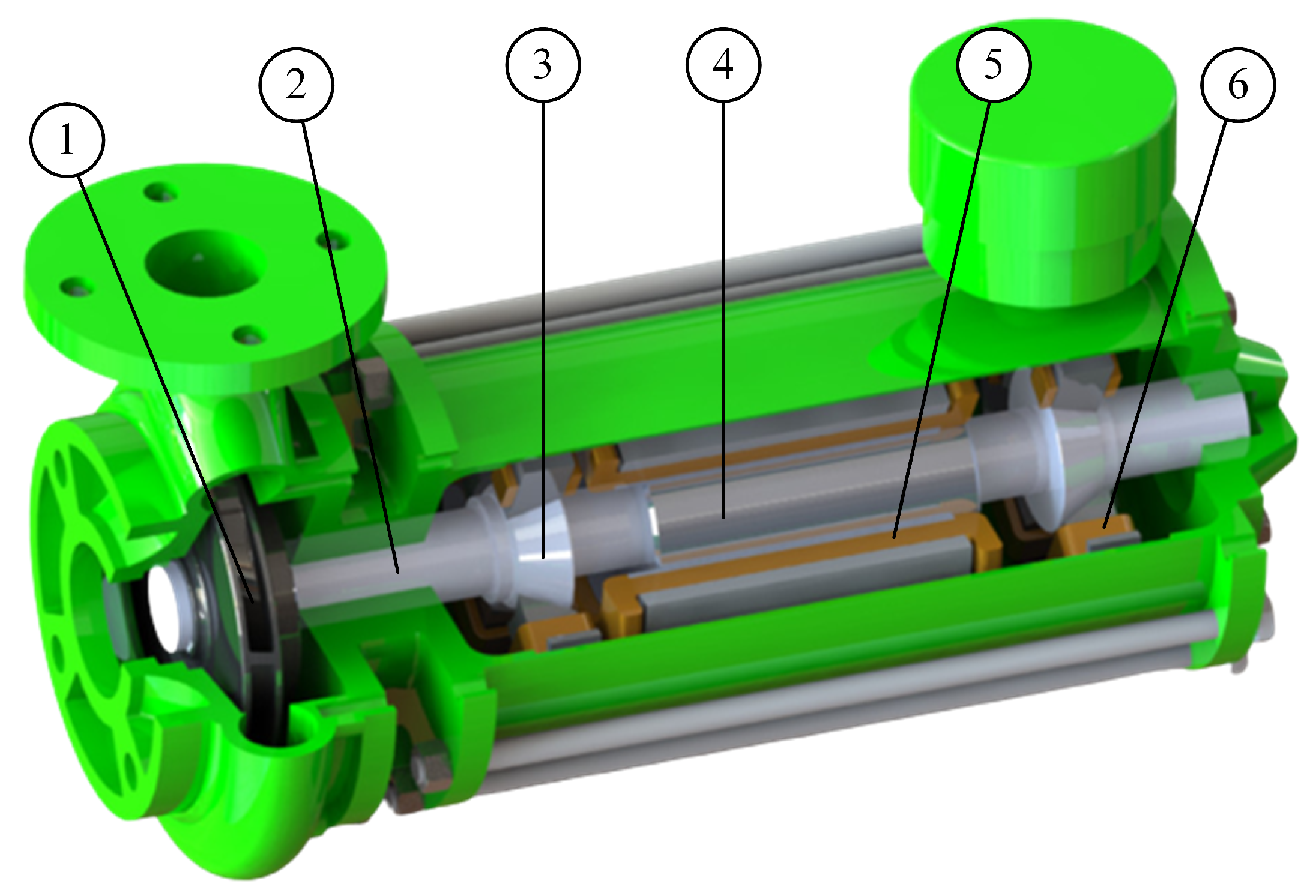
2. System Description and Modeling

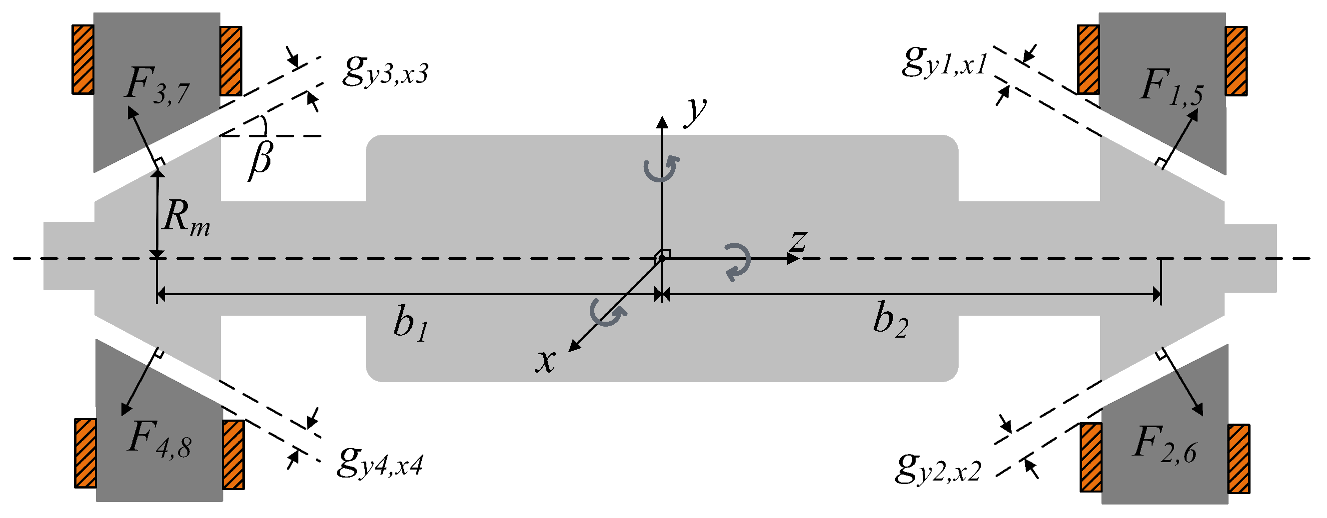
2.1. Fundamental Principle of Rigid Rotor Dynamics

The rigid rotor has five degrees of freedom, in which z, x, and y are the three radial translations, and the two rotational positions θ x , θ y are around the x and y axes, respectively. The rotor states are given by q = z x y θ x θ y T in the center of mass (COM) frame. The equations of motion are generalized in matrix form for an axially symmetric rotor rotating at a constant speed and are given by
M q ¨ + ( G + C b ) q ˙ + ( K + K b ) q = f ( t )
where M , G , and K denote the nominal parameter values of symmetric mass, skew-symmetric gyroscopic, and symmetric stiffness matrices, respectively. The gyroscopic matrix G is proportional to rotor spin speed Ω [41]. For AMBs, the matrix K   =   0 , because there is no physical contact between the rotor and a stationary mechanical bearing. The hydrodynamic effects of the fluid film between the rotor and the stator act on rotor dynamics through the damping matrix C b and the stiffness matrix K b ; f(t) is a forcing function including the CAMB suspension forces.
In the development of rigid body dynamics, the sensor coordinate of the rotor centerline located at the CAMB is determined by q b   =   z x 1 y 1 x 2 y 2 T . To transform between two coordinate frames, the transformation matrix T is given by q b = Tq
T = 1 0 0 0 0 0 1 0 0 b 1 0 0 1 b 1 0 0 1 0 0 b 2 0 0 1 b 2 0

2.2. Conical Active Magnetic Bearing Model

2.2.1. Electromechanical Interaction

The forces F 1 , . . . , F 8 generated by the active magnetic bearings are integrated into the rotor dynamics. They enter the rotor equations of motion through the input term f (t) of Equation (1) as the forces created by each bearing. Figure 2 shows the simple model of conical active magnetic bearings. Table 1 lists the parameters of the system.
The equations of motion can be written as following Newton’s second law and Euler’s second equations:
m z ¨ =   ( F 1 + F 2 + F 5 + F 6 ) sin β ( F 3 + F 4 + F 7 + F 8 ) sin β m x ¨ =   ( F 5 F 6 + F 7 F 8 ) cos β m y ¨ =   ( F 1 F 2 + F 3 F 4 ) cos β m g J d θ ¨ x =   [ ( F 1 F 2 ) b 2 + ( F 4 F 3 ) b 1 ] cos β + ( F 2 F 1 + F 3 F 4 ) R m sin β J p θ ˙ y Ω J d θ ¨ y =   [ ( F 6 F 5 ) b 2 + ( F 7 F 8 ) b 1 ] cos β + ( F 5 F 6 + F 8 F 7 ) R m sin β + J p θ ˙ x Ω
where J p θ ˙ y Ω and J p θ ˙ x Ω are additional components of the feedback force caused by gyroscopic action based on the law of angular momentum. In order to linearize Equation (2), the dynamic equation of the air gap can be written as follows considering the small motions of the rotor:
g y 1 , 2   =   g o z sin β ( y + b 2 θ x ) cos β g y 3 , 4   =   g o + z sin β ( y b 1 θ x ) cos β g x 1 , 2   =   g o z sin β ( x b 2 θ y ) cos β g x 3 , 4   =   g o + z sin β ( x + b 1 θ y ) cos β

2.2.2. Electromagnetic Forces

Assume that the reluctance of the iron is neglected concerning gap reluctance [42]. In addition, all magnets have identical structures and the fringing effect can be neglected [43]. The electromagnetic forces are given by:
F j = K I 2 g 2 , j = 1 , . . . , 8
The force coefficient is given as follows:
K = μ 0 N 2 A 4
where μ 0   =   4 β     H   ·   m 1 is the air permeability. In terms of the actual air gap and the current, the change in magnetic force can be written as follows:
F 1 , 3 = K ( I 01 + i y 1 , 3 ) 2 g y 1 , 3 2 F 5 , 7 = K ( I 01 + i x 1 , 3 ) 2 g x 1 , 3 2 F 2 , 4 = K ( I 02 + i y 2 , 4 ) 2 g y 2 , 4 2 F 6 , 8 = K ( I 02 + i x 2 , 4 ) 2 g x 2 , 4 2
where i q j ( j = 1 , 4 and q = y , x ) are the control currents of each magnet. Assume that the displacement of the rotor and the current change is small relative to the nominal air gap and bias current I 0 . Substituting Equation (3) into Equation (6), the magnetic force can be linearized as follows by using the Taylor series expansion. By choosing suitable approximations, second-order terms can be neglected, yielding a linear approximation to the function:
F 1 = F o 1 + K i 1 i y 1 + K q 1 z sin β + K q 1 ( y + b 2 θ x ) cos β F 2 = F o 2 + K i 2 i y 2 + K q 2 z sin β K q 2 ( y + b 2 θ x ) cos β F 3 = F o 1 + K i 1 i y 3 K q 1 z sin β + K q 1 ( y b 1 θ x ) cos β F 4 = F o 2 + K i 2 i y 4 K q 2 z sin β K q 2 ( y b 1 θ x ) cos β F 5 = F o 1 + K i 1 i x 1 + K q 1 z sin β + K q 1 ( x b 2 θ y ) cos β F 6 = F o 2 + K i 2 i x 2 + K q 2 z sin β K q 2 ( x b 2 θ y ) cos β F 7 = F o 1 + K i 1 i x 3 K q 1 z sin β + K q 1 ( x + b 1 θ y ) cos β F 8 = F o 2 + K i 2 i x 4 K q 2 z sin β K q 2 ( x + b 1 θ y ) cos β
where F 0 j = K I 0 j 2 g 0 2 ,   j = 1 , 2 are the steady-state magnetic forces and K q j = 2 F 0 j g 0 ,   K i j = 2 F 0 j I 0 j ,   j = 1 , 2 are the position and current stiffnesses.

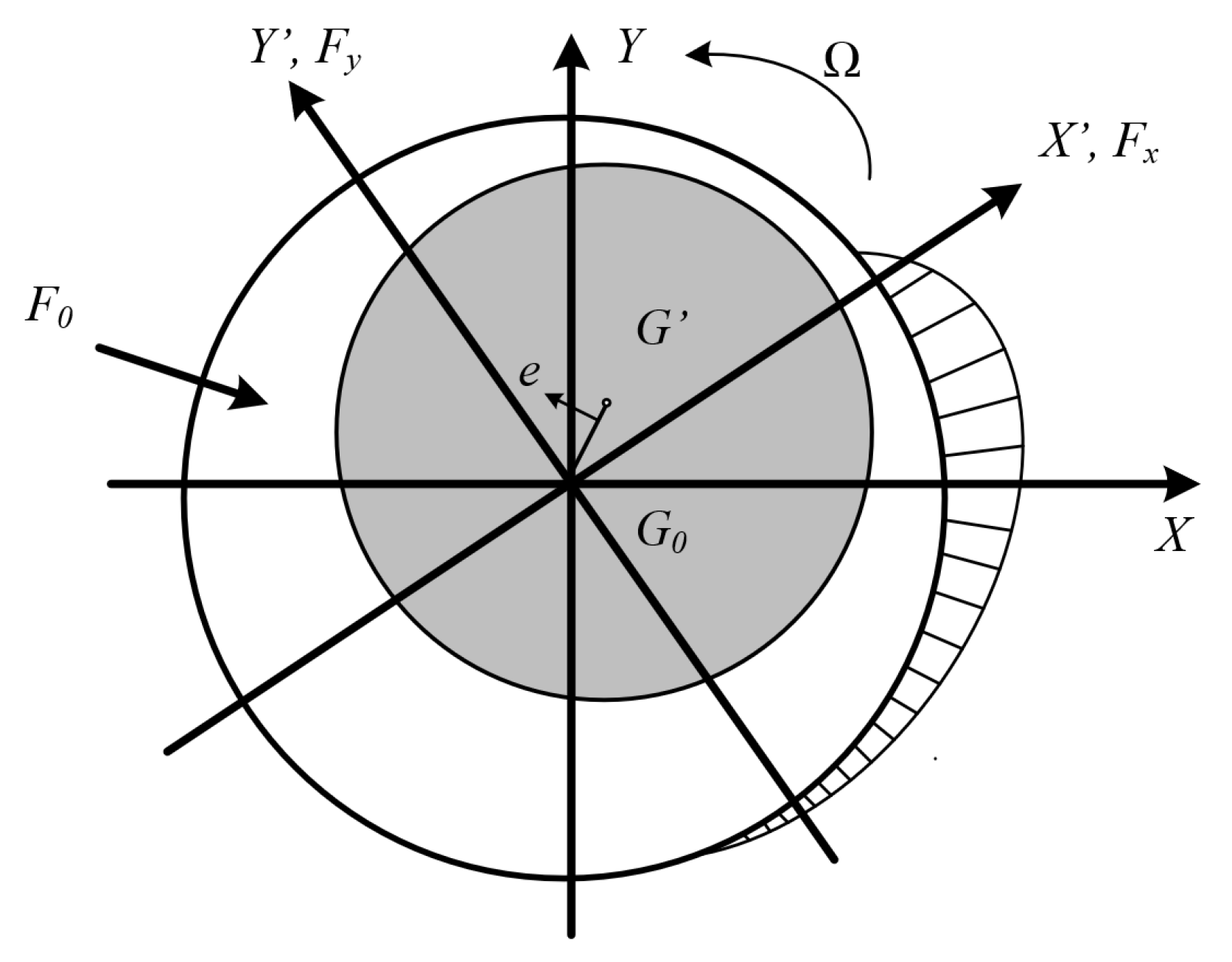
2.3. Hydrodynamic Forces

As an absolutely leak-proof safety pump, a canned motor pump requires a more complicated and clever design. The rotor is completely surrounded by a hermetically sealed can with a thin fluid layer between the rotor can and the stator can. However, this causes whirling of the rotor, which can become more serious at high speed. In addition, hydrodynamic interactions generate cross-coupling forces between the radial axes of significant magnitude. This phenomenon, which is the main cause of system instability, is far more complex and cannot be neglected.
The hydrodynamic force amplitude is not significant during normal operation and is only brought on by the velocity difference between the cans of the rotor and stator. However, forces on the impeller, mass imbalances in the motor, and external disturbances all cause the rotor to wander slightly away from its geometric center, which immediately causes radial hydrodynamic forces to act on the rotor. These forces depend on the rotor’s rotational speed and movement. The hydrodynamic forces can be described by the dimensionalized stiffness and damping matrices coefficients K i j and C i j , respectively [44]. Their interaction with the axial force on the rotor is given by:
F x F y = C 11 C 12 C 21 C 22 x ˙ y ˙ + K 11 K 12 K 21 K 22 x y
The coefficients are derived as non-dimensional coefficients to simplify the derivation of the stiffness and damping matrices. The relationships between them are given by:
K i j = F 0 g 0 K i j * , C i j = F 0 g 0 Ω C i j * , i , j = 1 , 2
F 0 = F μ S * = μ L 3 Ω R m 2 g 0 2 ε π 2 π 2 ε 2 + 16 ε 2 2 ( 1 ε 2 ) 2
where g 0 denotes the nominal space between the cans of the rotor and the stator; F 0 / F μ is referred to as the bearing Summerfield number; F 0 is the static force; e = ε g 0 = x 2 + y 2 and 0 ε 1 is the eccentricity ratio referred to Figure 3; μ is the absolute viscosity; L, R m , and Ω are the length of the rotor, the radius of the rotor, and the angular velocity, respectively.
The values of the non-dimensional stiffness and damping matrix are given by [44]. The hydrodynamic forces only act in the radial motion of the rotor and have no effect on the rotation of the rotor axis about the z-axis. Hence, the hydrodynamic force equations in the AMB coordinate system can be written as follows:
F z F x 1 F y 1 F x 2 F y 2 = 0 0 0 0 0 0 K 11 K 12 0 0 0 K 21 K 22 0 0 0 0 0 K 11 K 12 0 0 0 K 21 K 22 z x 1 y 1 x 2 y 2 + 0 0 0 0 0 0 C 11 C 12 0 0 0 C 21 C 22 0 0 0 0 0 C 11 C 12 0 0 0 C 21 C 22 z ˙ x ˙ 1 y ˙ 1 x ˙ 2 y ˙ 2
F b = K b q b + C b q ˙ b
Finally, they are transformed into the COM coordinate system by:
F = T T F b = T T ( K b Tq + C b T q ˙ )

2.4. CAMB with Lumped Disturbances

In the COM coordinate system, Equations (2), (7), and (13) are combined to describe the motion of the rotor. After the appropriate transformations are applied, the model in COM coordinate is given by
M + Δ M q ¨ + ( G + Δ G + T T C b T ) q ˙ + ( K c + Δ K c + T T K b T ) q = K i b m i m
where Δ M , Δ G , and Δ K c represent parameter uncertainties of symmetric mass, skew-symmetric gyroscopic, and symmetric stiffness matrix, respectively.
q = { z , x , y , θ x , θ y } T i m = { i y 1 , i y 2 , i y 3 , i y 4 , i x 1 , i x 2 , i x 3 , i x 4 } T
M = m 0 0 0 0 0 m 0 0 0 0 0 m 0 0 0 0 0 J d 0 0 0 0 0 J d G = 0 0 0 0 0 0 0 0 0 0 0 0 0 0 0 0 0 0 0 J p θ z . 0 0 0 J p θ z . 0
K i b m = K i 1 sin β K i 1 cos β 0 0 K i 1 σ K i 2 sin β K i 2 cos β 0 0 K i 2 σ K i 1 sin β K i 1 cos β 0 0 K i 1 γ K i 2 sin β K i 2 cos β 0 0 K i 2 γ K i 1 sin β 0 K i 1 cos β K i 1 δ 0 K i 2 sin β 0 K i 2 cos β K i 2 δ 0 K i 1 sin β 0 K i 1 cos β K i 1 γ 0 K i 2 sin β 0 K i 2 cos β K i 2 γ 0 T
K c = K 11 0 0 K 14 K 15 0 K 22 0 0 K 25 0 0 K 33 K 34 0 K 41 0 K 43 K 44 0 K 51 K 52 0 0 K 55
δ = b 2 cos β R m sin β γ = b 1 cos β + R m sin β σ = b 2 cos β R m sin β
K 11 = 4 ( K q 1 + K q 2 ) sin 2 β K 14 = K 15 = ( b 1 + b 2 ) ( K q 1 K q 2 ) sin β cos β K 22 = K 33 = 2 cos 2 β ( K q 1 + K q 2 ) K 25 = K 52 = K 34 = K 43 = cos 2 β ( K q 1 + K q 2 ) ( b 1 b 2 ) K 41 = K 51 = sin β ( K q 1 K q 2 ) ( b 1 + b 2 ) cos β 2 R m sin β ) K 44 = K 55 = cos β ( K q 1 + K q 2 ) ( b 1 2 + b 2 2 ) cos β R m ( b 1 + b 2 ) cos β )
It can be seen that only the mass matrix has components that are on the major diagonal, the system’s equation is intricate and coupled. This feature prevents the normally linear controller from being applied in all motion directions. In order to reject coupling effects, the FOADRC method treats them as system disturbances.

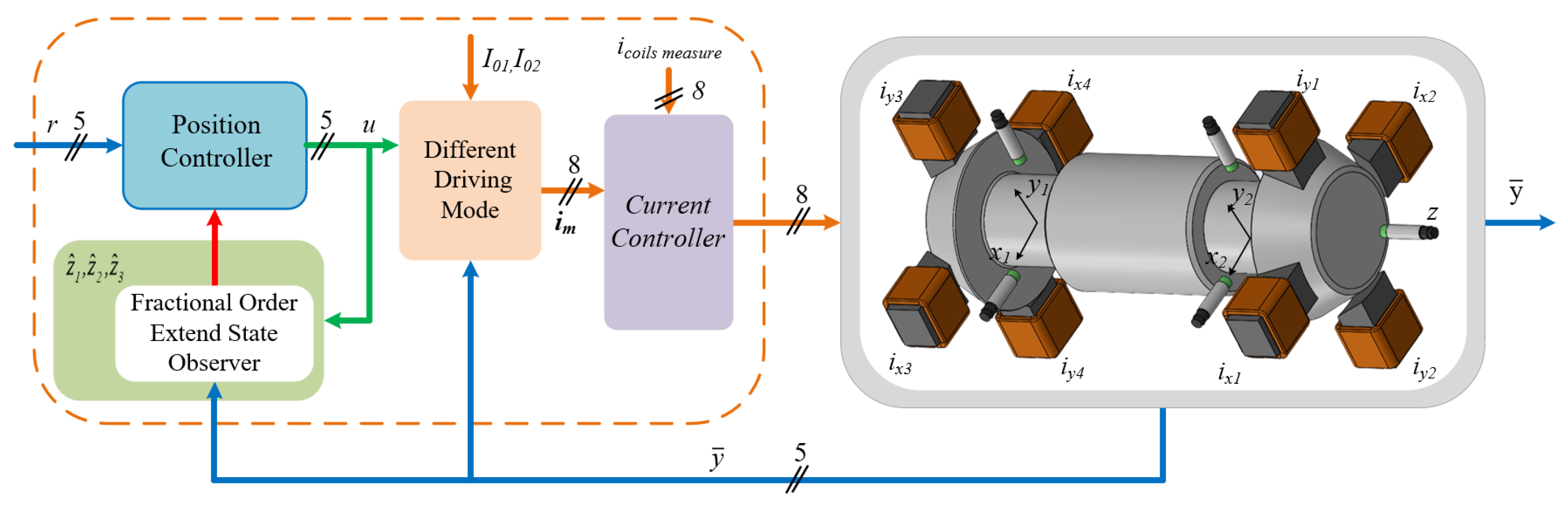
2.5. Driving Current Structure

Every magnetic pole pair of the CAMB can provide both the axial force and radial force to the rotor; it constitutes an inherently unstable system. The stabilizing control of the electromagnet current is necessary to find a solution for this issue. The coil current of the system operating in differential driving mode is employed to control the rotor. The general principle is one electromagnet is driven with the sum of a bias and a control current, whereas the opposite one is driven with their difference. By increasing the forces on the lower bearings and reducing the forces on the upper bearings in Figure 2, any positive movement along y away from the equilibrium point can be compensated for. The goal of this control strategy is to sustain levitation and maintain the rotor position at the center of the stator with only the bias current present on each magnetic pole pair. Five virtual control currents are used to control the five-DOF plant. The following is how the currents passing through the coils are expressed:
i y 1 i y 2 i y 3 i y 4 i x 1 i x 2 i x 3 i x 4 = I o 1 I o 2 I o 1 I o 2 I o 1 I o 2 I o 1 I o 2 + 1 0 0 0 1 1 0 0 0 1 1 0 1 0 0 1 0 1 0 0 1 0 0 1 0 1 0 0 1 0 1 1 0 0 0 1 1 0 0 0 H I z I x 1 I y 1 I x 2 I y 2
where I 0 = I 01 I 02 I 01 I 02 I 01 I 02 I 01 I 02 T is the bias current. At steady-state, consider I 0 = 0 , i r = I z I x 1 I y 1 I x 2 I y 2 T are the five virtual control currents. For this situation, Equation (14) can be rewritten as:
M + Δ M q ¨ + ( G + Δ G + T T C b T ) q ˙ + ( K c + Δ K c + T T K b T ) q = K i b m H i r
Equation (14) has shown the object model in linear form, there is still an inter-channel component between the control variables, so in this part, the decoupling technique will be used to reduce them and the amount of computation as well as increase the accuracy of the FOADRC controller. The K c and K i b m H are invertible. The interstitial component can be reduced by using the following control structure:
i r = ( K i b m H ) 1 ( v + K c T 1 q b )
Equation (16) can be rewritten as
M q ¨ + ( Δ M q ¨ + ( G + Δ G + T T C b T ) q ˙ + ( Δ K c + T T K b T ) q ) D ( q ¨ , q ˙ , q , t ) = v
where D q ¨ , q ˙ , q , t denotes the lumped disturbances of CAMB including the external disturbances f , the parameter uncertainties, and the coupling components; v is the new control signal. We have the linear version of the system presented in Equation (18) with five inputs and five outputs due to linearity and decoupling. Equation (18) shows that the gyroscopic force and hydrodynamic impact cause the interchannel component of the model to persist in the control channel. The control object is then stabilized, and the remaining interstitial components are removed using the FOADRC.

3. Lumped Disturbances Rejection Control Design

3.1. Preliminaries and Problem Formulation
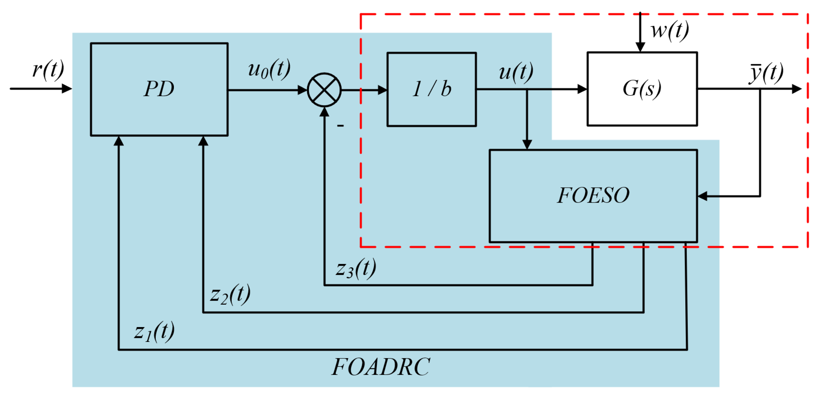
Many studies in the literature present different definitions of fractional-order derivatives; Caputo’s definition is usually used by engineers. The fractional derivative of a fractional order is defined by Caputo [45] with variable t 0 = 0 and starting point as in
D α f ( t ) = 1 Γ n α 0 t f ( n ) ( τ ) t τ α + 1 n d ( τ )
where Γ ( x ) is Euler’s gamma function and n is an integer satisfying n 1 α n , f n τ is the n derivative of the f ( τ ) . The following characteristic function with commensurate order α of a linear fractional system [46] is represented by the transfer function model as
D ( s ) = a n s n α + a n 1 s ( n 1 ) α + + a 1 s α + a 0
Denoting ω = s α , Equation (20) becomes
D ( ω ) = a n ω n + a n 1 ω ( n 1 ) + + a 1 ω + a 0
Lemma 1.
In [46], the fractional order system with the characteristic function (20) is BIBO stable if and only if all poles ω i of the polynomial (21) satisfy | arg ( ω i ) | > ( α π ) / 2 , i = 1 , 2 , , n .
The stability zone of the commensurate fractional-order system in the ω plane is depicted in Figure 4; two boundary lines for the stable region has the slope with ± α π / 2 [47]. The stable region includes the left half-plane, including the imaginary axis because 0 < α < 1 . The fractional-order of the s plane is transferred to the integer-order system of the ω plane using the mapping relation ω = s α , where α is the initial system’s order. The correlation between the trajectory and the stable region of the ω plane can be used to determine how stable the initial fractional-order system is. If all the poles of the mapped integer order system about ω are determined at the left half-plane, the system is stable; otherwise, it is unstable.

3.2. FOADRC Design

In this paper, a FOADRC including a FOESO and PD controller is proposed, and the structure of the FOADRC is shown in Figure 5. The second order system is given as follows:
P ( s ) = Y ( s ) U ( s ) = b s 2 + a 1 s + a 2
Considering the external disturbance w, Equation (22) can be rewritten as follows:
y ¯ ¨ = a 1 y ¯ ˙ a 2 y ¯ + w + b u
where a 1 , a 2 , and b are constants, and y ¯ and u are the output and input, respectively. The second integer order model can be converted into a cascaded fractional order integrator platform as follows:
y ¯ ( 2 α ) = f ( y ¯ ( 2 α ) , y ¯ ¨ , y ¯ ˙ , y ¯ , w ) + b u
where f is referred to as the generalized disturbance including external disturbance w, fractional dynamics y ¯ 2 α where 0 < α < 1 , and unknown dynamics. Only the order of the system and parameter b are known; the control input is defined as u.
The idea of ESO is to estimate the total disturbance through an extended state and compensate for it. ESO can determine the total disturbing forces affecting the active magnetic bearing system by measuring the rotor output displacement and the controller output. Let x ¯ 1 = y ¯ , x ¯ 2 = y ¯ ( α ) , and x ¯ 3 = f , where x ¯ 1 and x ¯ 2 represent system states and x ¯ 3 represents the external state. The state equation of Equation (24) is defined as follows:
x ¯ 1 ( α ) = x ¯ 2 x ¯ 2 ( α ) = x ¯ 3 + b u x ¯ 3 ( α ) = h y ¯ = x ¯ 1
States estimation in Equation (25) is achieved through the FOESO as follows:
z 1 ( α ) = z 2 + β 1 ( y ¯ z 1 ) z 2 ( α ) = z 3 + b u + β 2 ( y ¯ z 1 ) z 2 ( α ) = β 3 ( y ¯ z 1 ) y ¯ ^ = z 1
where L = β 1 β 2 β 3 T are observer gains indicated by the displacement, speed, and disturbance feedback gain; z 1 z 2 , and z 3 are outputs of FOESO and the estimation of the state x ¯ 1 , x ¯ 2 , x ¯ 3 , respectively.
The disturbance compensation link adjusts the control volume as determined by state error feedback when the FOESO can estimate an extended state. Then, to reject f ( t ) , the control law can be designed as follows:
u = z 3 + u 0 b
In order to achieve the desired response, a controller with proportional and derivative actions is designed as follows:
u 0 = k p ( r z 1 ) + k d ( z 2 )
Note that k d z 2 is used instead of k d ( r ˙ z 2 ) to avoid the differentiation of the set value, which also prevents the AMB’s system problems caused by the rapid change of the set value. The perturbed system is approximately converted into a fractional order integrator as follows:
y ¯ ( 2 α ) = u 0 + ( f f ^ ) u 0

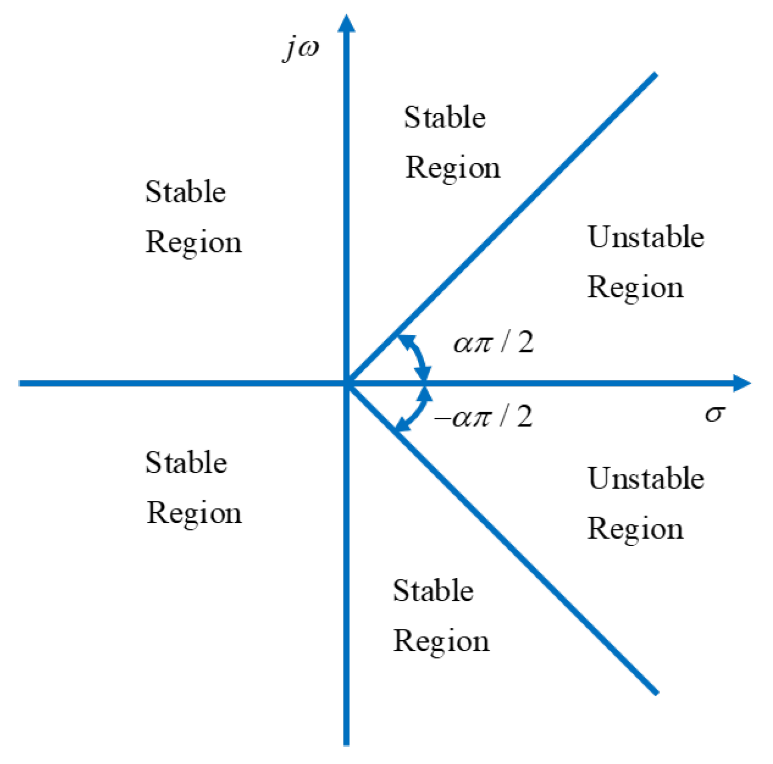
3.3. Stability Analysis and Parameter Tuning

The error equation combining Equations (25) and (26) can be written as
e ( α ) = A e e + E h
where
A e = β 1 1 0 β 2 0 1 β 3 0 0 , E = 0 0 1 , e = e 1 e 2 e 3 = x ¯ 1 z 1 x ¯ 2 z 2 x ¯ 3 z 3
Theorem 1.
The FOADRC design from Equation (26) to Equation (29) is bounded-input bounded-output (BIBO) stable closed-loop system if the observer in Equation (26) and L and the state feedback control law are stable, respectively.
Proof.
If the error equation converges, the poles should be placed in the stable area of the graph according to the bandwidth parameter approach of the integer-order extended state observer. Since 0 < α < 1 , it is obvious that the left half-plane of s is where the root locus of its transfer function resides. In other words, the entire left half of the plane is covered by the stable zone. For linear FOESO parameter adjustment, the integer-order ESO bandwidth tuning approach is acceptable. Therefore, it is possible to employ the observer bandwidth ω o concept put out by professor Gao Zhiqiang [18]. The characteristic function of error Equation (30) is
F ( s ) = s 3 α + β 1 s 2 α + β 2 s α + β 3
The observer gains are chosen such that the characteristic polynomial is Hurwitz. For convenience, all the observer poles are placed at ω o 1 / α , with ω o > 0 , that is, F ( s ) = ( s α + ω o ) 3 . Hence, the parameters β 1 = 3 ω o , β 2 = 3 ω o 2 , β 3 = ω o 3 ensure A e is a Hurwitz matrix. The fractional-order extended state observer’s parameter adjustment procedure is straightforward because the bandwidth ω o and the parameters that need to be altered are directly related. Under the zero initial conditions, the transfer function from h ( t ) to e i ( t ) is calculated as
G ( s ) = s α + β 1 1 0 β 2 s α 1 β 3 0 s α 1 0 0 1
By using the final value theorem, we have
e 1 ( + ) e 2 ( + ) e 3 ( + ) = lim s 0 s G ( s ) h ( s ) = 1 / β 3 β 1 / β 3 β 2 / β 3 h ( + )
Assuming h is bounded, i.e., | h + | M , we obtain
e i ( + ) 1 / β 3 β 1 / β 3 β 2 / β 3 M
The upper bounds of the estimate errors are given by Equation (34). With A e being Hurwitz and h bounded, FOESO is asymptotically BIBO stable via Lemma 1. □
Remark 1.
The state and extended state of the fractional-order object can be precisely observed using the fractional-order extended state observer. Additionally, FOESO’s resistance to parameter changes is strengthened. Instead of using integer-order controllers, fractional-order controllers are utilized to manage the position feedback error rate, resulting in a wider range of adjustment for the feedback control law and a more effective control signal.
Referring to Equations (27)–(29), the required response of FOADRC may be derived as the following closed-loop transfer function:
G d ( s ) = Y ( s ) R ( s ) k p s 2 α + k d s α + k p
The stability of the closed-loop system (refer to Equation (35)) using FOADRC is determined by the characteristic function H ( s ) = s 2 α + k d s α + k p . For tuning simplicity, the closed-loop characteristic polynomial has two poles at ω c 1 / α . Here, the parameter adjustment is further simplified as k p = ω c 2 , k d = 2 ω c , where ω c is the ω -plane bandwidth of the controller. Thus, the closed loop is BIBO stable.
In general, a larger ω -plane bandwidth results in a faster reaction, but it may push the system to its limit, leading to oscillations or even instability. As a result, a well-tuned ω must achieve a balance between rapidity and stability. By applying the tuning method in [48], the controller bandwidth is tuned via the settling time. By choosing the controller gain as k p = ω c 2 , k d = 2 ω c , the closed-loop transfer function becomes
G d ( s ) = ω c 2 ( s α + ω c ) 2
The tuning method presented in [48] uses the settling time t s and the overshoot σ % to determine controller bandwidth. If the overshoot of Equation (36) is constantly zero, t s turns into the main factor considered when picking ω c . Therefore, one practical approach with a desired 2 % settling time is used to derive the relation between t s and ω c . Under a unit step change in the input signal, the output of Equation (36) is
Y ( s ) = ω c 2 s ( s α + ω c ) 2
The inverse fractional Laplace transform of Equation (37) is given as
y ¯ ( t ) = 1 E α ( ω c t α ) ω c t α 1 E α , α ( ω c t α )
where E is Mittag-Leffler function. According to the definition of setting time
| y ¯ ( t s ) y ¯ ( ) | = Δ
where y ¯ ( ) =1 and Δ = Δ 2 % , we have
| y ¯ ( t ) 1 | = 0.02
By solving Equations (38)–(40), ω c can be determined as follows:
t s = 3.3265 ω c
As a result, the desired dynamic characteristic of the system is decided. However, the actual output, due to some factors, cannot achieve the desired dynamic characteristic. Therefore, some margins are required to ensure the design’s reliability [48]. In this paper, ω c is determined as following ω c = 6 / t s . With the observer bandwidth set as a multiple of the controller bandwidth ω o = 5 10 ω c [18], the entire system is tuned by adjusting the controller bandwidth.

4. Numerical Simulation Study

4.1. Simulation Settings

In this section, we consider three scenarios using the MATLAB/Simulink environment to compare and evaluate the efficacy of FOADRC, ADRC, and PID controllers in the presence of variable rotation speed, rotor load disturbance, measurement noise, and hydrodynamic force. Then, from the initial values of the rotor center of mass position, the controller is used to drive the rotor’s five axes to a set point of 0. The initial values of the rotor center of mass position are z 0 = 0.2   ×   10 3 m ;   x 1 0 = 0.2   ×   10 3 m ;   y 1 0 = 0.2   ×   10 3 m ;   x 2 0 = 0.2   ×   10 3 m ;   y 2 0 = 0.2   ×   10 3 m . The selected coefficients of the FOADRC are listed in Table 2.
The control strategy of the CAMB in a canned motor pump, presented in Figure 6. Position sensors measure the difference between the desired and actual rotor positions and transmit these data to the FOESO and the structure “different driving mode”. The control signal is then calculated using the FOESO and position controller. The control signal and available information are used by the current controller to change the attraction force for the electromagnets in order to change the position of the rotor. In order to evaluate the performance of the proposed control system compared with conventional ADRC and PID for CAMB, three scenarios are expressed as follows:
Scenario 1:
The rotating rotor of the conical active magnetic bearing is not spinning around the z-axis, and the rotor deviates from the equilibrium position at the initial time under the parameter uncertainties including Δ M , Δ G , and Δ K c (i.e., the actual parameters of CAMB deviate about 10% from the nominal value).
Scenario 2:
The rotor is brought to the equilibrium position at the initial time. Then, it rotates at normal speed (3000 rpm), and the conical active magnetic bearing is affected by the parameter uncertainties (i.e., the actual parameters of CAMB deviate about 10% from the nominal value) and the external disturbances (i.e., the hydrodynamic vibrations of the canned motor that are detailed in the Section 2.3).
Scenario 3:
The rotor is brought to the equilibrium position at the initial time. Then, it rotates at high speed (12,000 rpm) in case the hydrodynamic force is applied. The conical active magnetic bearing is affected by the disturbances, including the parameter uncertainties and the external disturbances. In addition, the measurement noise created by white Gaussian noise is added to the rotor states to demonstrate the performance of the proposed control system.

4.2. Results and Discussion

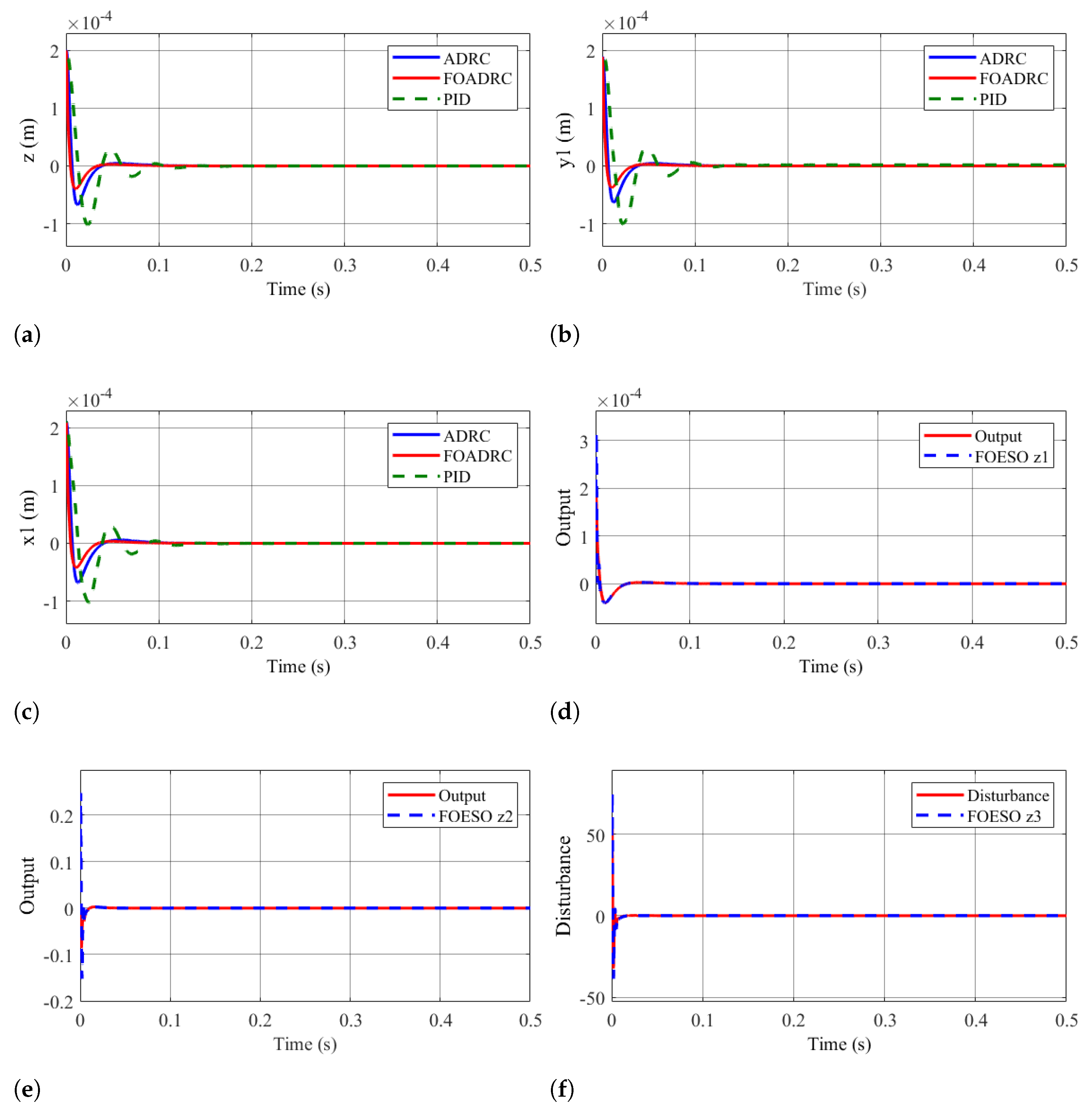
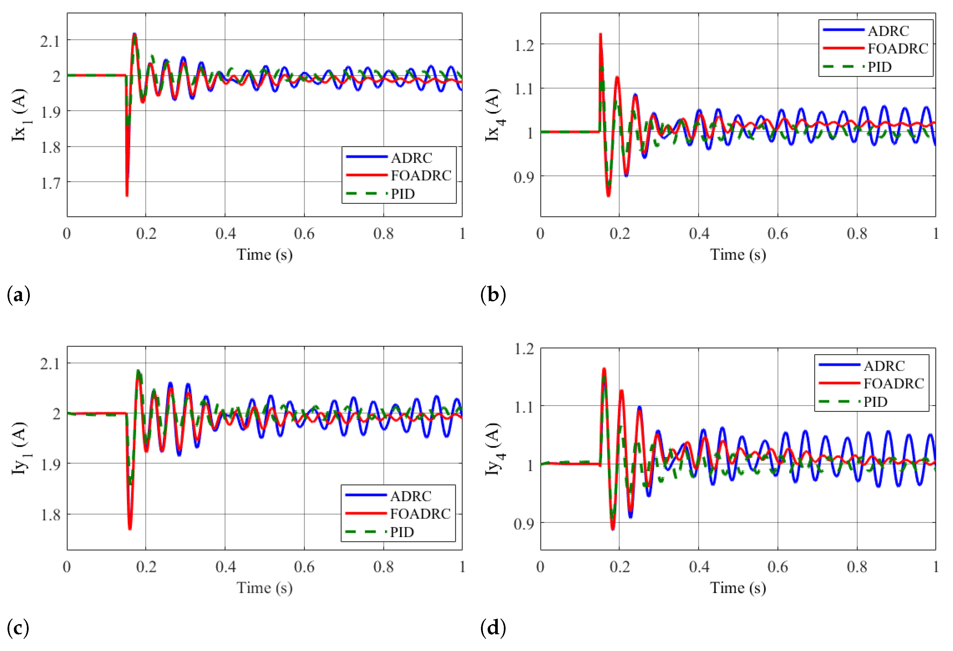
4.2.1. Results of Scenario 1

The performance of the FOADRC controller is verified and compared with PID and ADRC controllers. The FOADRC system’s position response achieves no fluctuation, a shorter settling time, and a small overshoot peak, as shown in Figure 7a–c. As a result, the FOADRC controller shows superior controllability compared to the ADRC and PID controllers when the rotor is not spinning around the z-axis and is deviated from the equilibrium position.
Based on Figure 7d–f, the FOESO can track the disturbance and actual values in a remarkably short period of time (0.02 s). The FOESO provides observation quality, ensures control quality, and sees good response performances when parameter uncertainties are presented.
The required levitation control currents in upper and lower coils computed by the FOADRC, ADRC, and PID controllers are shown in Figure 8. Unlike the PID controller’s current, the FOADRC controller’s current rapidly brings the rotor to equilibrium, with only bias current flowing through each coil.

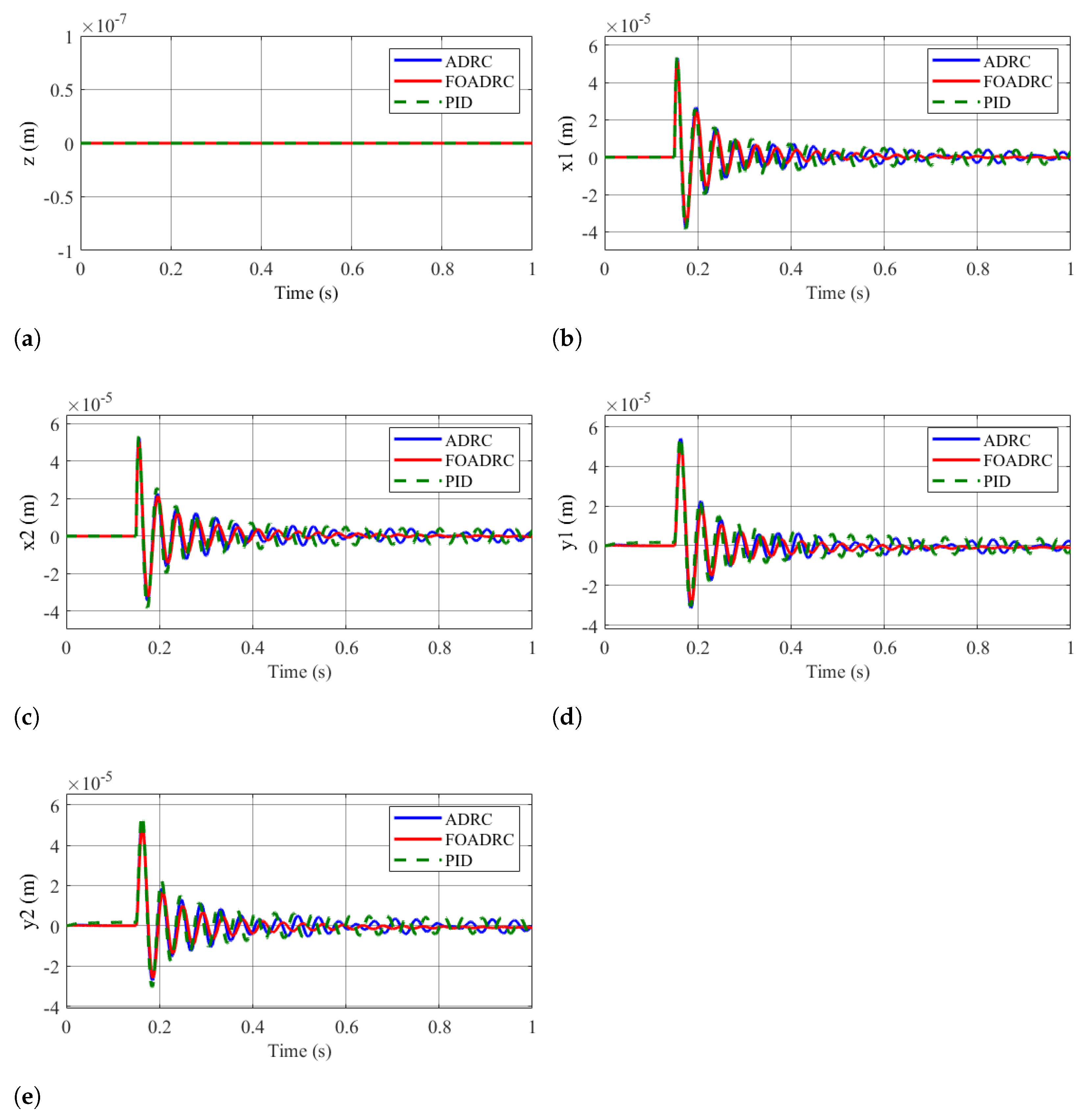
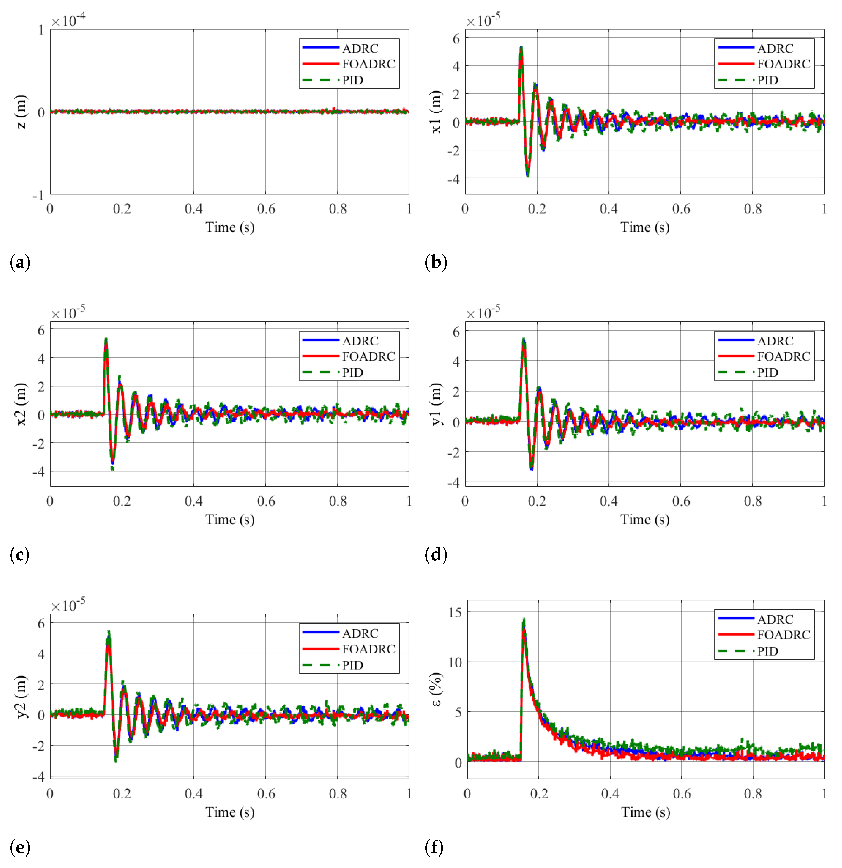
4.2.2. Results of Scenario 2

The rotor speed is set to 3000 rpm, and the rotor is brought to equilibrium at the start. At 0.15 s, hydrodynamic forces make contact with the rotor. With the hydrodynamic forces applied to the rotor, the FOADRC system achieves lower overshoot, fluctuation, and a faster settling time, as shown in Figure 9a–e. The position of the rotor oscillates around the equilibrium point with the FOADRC controller and has a stability state of 0.8 s. As shown in Figure 9, the PID and ADRC controllers can keep the rotor oscillating close to the equilibrium position and cannot fully bring the rotor to equilibrium. These results show that the FOADRC controller has faster response times and better vibration-damping ability than ADRC and PID controllers when the rotor is operated under hydrodynamic forces.
Figure 10 shows the responses of typical direct control currents in systems controlled by FOADRC, ADRC, and PID. As can be seen, when the system is under the influence of hydrodynamic force, the control currents generated by the FOADRC controller are quite large but still within the allowable limit. The main reason is that the FOADRC controller is quite sensitive to uncertainties and external disturbances. The FOADRC control current quickly brings the rotor into equilibrium and remains stable around the bias current with very little oscillation, whereas the control currents generated by ADRC and PID controllers fluctuate significantly around the bias current.

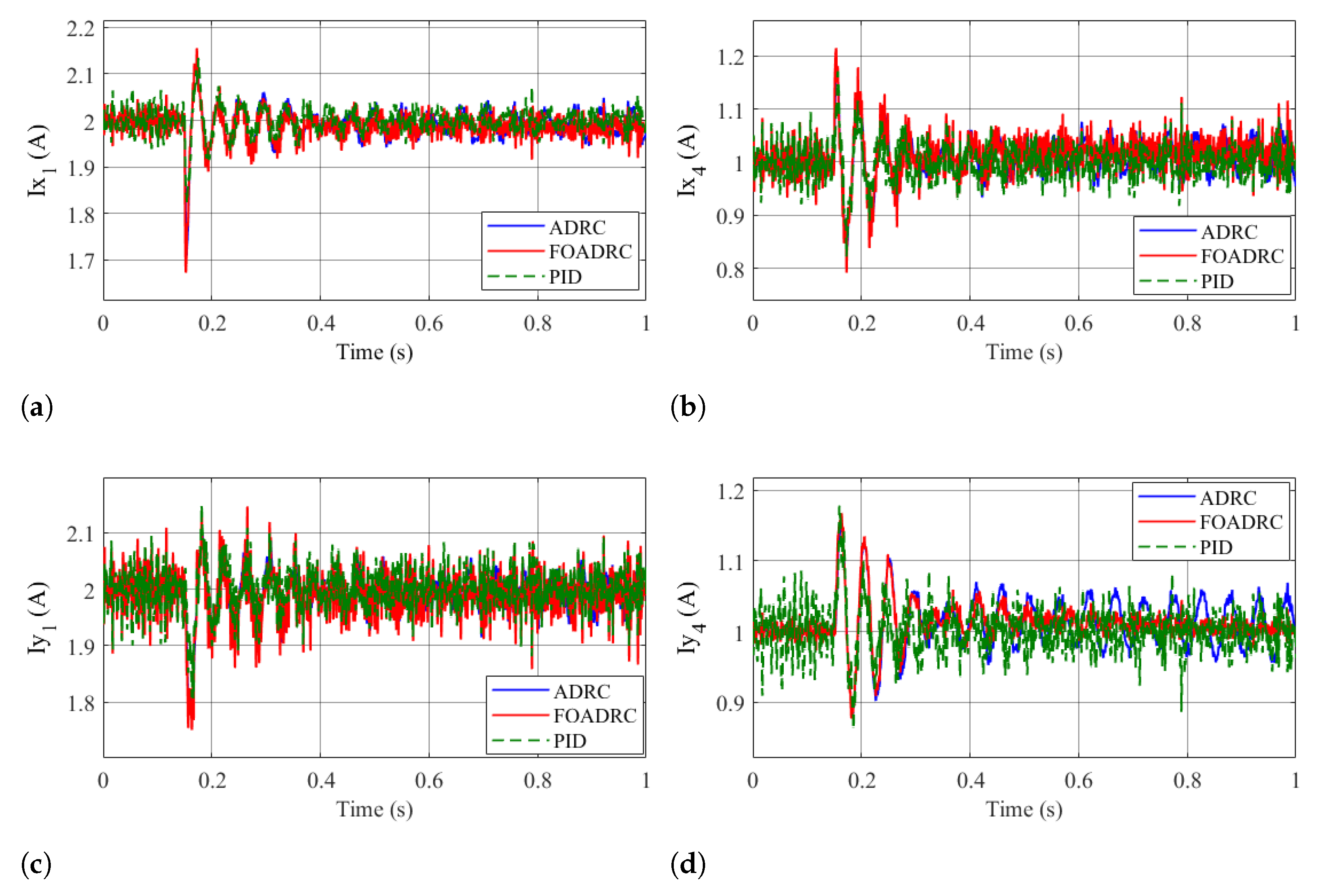
4.2.3. Results of Scenario 3

The rotor speed is initialized to 12,000 rpm to evaluate the performance of controllers when the rotor is in the high-speed region under hydrodynamic force. The rotor is brought to the equilibrium position at the initial time. Then, hydrodynamic forces contact the rotor at 0, 15 s. This simulation scenario includes measurement noise. As shown in Figure 11a–e, the simulation results on the z , x 1 , y 1 , x 2 , and y 2 axes are similar to those obtained in the second simulation scenario. When the rotor rotates at high speed, under the action of hydraulics and measuring noise, no axis of motion is significantly affected using the FOADRC controller. According to Figure 11f, when using the FOADRC controller, the eccentricity ratio of the rotor returns quickly and close to 0 after 0.6 s, whereas the PID and ADRC controllers show an eccentricity ratio close to 0 after a long time interval. The FOADRC controller has considered the rotor speed factor and shows its ability to resist measurement noise and work effectively in the high-speed region.
Figure 12 shows control currents where the rotor works in the high-speed region under hydrodynamic force and measurement noise. Similar to scenario 2, when starting to be under the influence of hydrodynamic force, the FOADRC control current is larger than the ADRC and PID control current but still within the allowable range. The FOADRC control current quickly brings the rotor into equilibrium, but it fluctuates more around the bias current than in scenario 2 because the rotor rotates at a fast speed and the system is influenced by measurement noise. When compared to ADRC and PID control, the FOADRC control current amplitude of oscillation is quite small and has no significant impact on rotor stability.
The closed-loop responses under PID, ADRC, and FOADRC control actions in terms of rotor state tracking errors are summarized in the following table.
It can be observed from Table 3 that, in the face of measurement noise, both FOADRC and ADRC performances deteriorate. This result is expected because the two controls are not designed to be robust to this type of noise. However, FOADRC still slightly out-performs ADRC.

5. Conclusions

The paper deals with the design integration of a cone-shaped magnetic bearing in a canned motor pump, which is characterized as a class of under-actuated and strongly coupling systems. The control strategy based on FOADRC combining FOESO and PD controller is suggested for improving the transient and steady performances and robustness with respect to parameter uncertainty and disturbance. Moreover, the convergence of the extended state observer and the stability of the proposed control strategy are proved. The simulation result is conducted and showed the effectiveness of the proposed controller, achieving superior performance and less sensitivity to noise measurement compared to the traditional ADRC and PID controller. In the near future, experiments considering the real-time implementation of the fractional system will be conducted to demonstrate the designed control structure thoroughly for real-life applications.

Author Contributions

Conceptualization: D.H.N., T.T.T., L.M.V., V.T.D., D.G.N., D.T.L., D.D.N. and T.L.N.; methodology: D.H.N., T.T.T., L.M.V., D.T.L. and T.L.N.; validation: D.H.N., T.T.T., L.M.V., V.T.D., D.G.N., D.T.L., D.D.N. and T.L.N.; data curation: D.H.N., T.T.T., L.M.V., V.T.D., D.G.N., D.T.L., D.D.N. and T.L.N.; writing—original draft preparation: D.H.N., T.T.T., L.M.V., D.T.L. and T.L.N.; writing—review and editing: D.H.N., T.T.T., L.M.V., V.T.D., D.G.N., D.T.L., D.D.N. and T.L.N.; supervision: T.L.N.; project administration, T.L.N.; funding acquisition: T.L.N. All authors have read and agreed to the published version of the manuscript.

Funding

This research received no external funding.

Institutional Review Board Statement

Not applicable.

Informed Consent Statement

Not applicable.

Data Availability Statement

The study did not report any data.

Conflicts of Interest

We declare that we have no conflict of interest.

References

  1. Nguyen, D.; Nguyen, L.; Hoang, D. A non-linear control method for active magnetic bearings with bounded input and output. Int. J. Power Electron. Drive Syst. 2020, 11, 2154. [Google Scholar] [CrossRef]
  2. Nguyen, T. Decoupling Control of a Disc-type Rotor Magnetic Bearing. Int. J. Integr. Eng. 2021, 13, 247–261. [Google Scholar] [CrossRef]
  3. Nguyen, D.; Nguyen, T.; Nguyen, M.; Nguyen, H. Nonlinear Control of an Active Magnetic Bearing with Output Constraint. Int. J. Electr. Comput. Eng. (IJECE) 2018, 8, 3666–3677. [Google Scholar] [CrossRef]
  4. Breńkacz, Ł.; Witanowski, Ł.; Drosińska-Komor, M.; Szewczuk-Krypa, N. Research and applications of active bearings: A state-of-the-art review. Mech. Syst. Signal Process. 2021, 151, 107423. [Google Scholar] [CrossRef]
  5. Li, X.; Palazzolo, A.; Wang, Z. A Combination 5-DOF Active Magnetic Bearing for Energy Storage Flywheels. IEEE Trans. Transp. Electrif. 2021, 7, 2344–2355. [Google Scholar] [CrossRef]
  6. Chiba, A.; Fukao, T.; Ichikawa, O.; Oshima, M.; Takemoto, M.; Dorrell, D. Magnetic Bearings and Bearingless Drives; Elsevier: Amsterdam, The Netherlands, 2005. [Google Scholar]
  7. Hantke, A.; Sobotzik, J.; Nordmann, R.; Brodersen, S.; Gröschel, J.; Köhler, B. Integration of Magnetic Bearings in a Canned Motor Pump. IFAC Proc. Vol. 2000, 33, 215–221. [Google Scholar] [CrossRef]
  8. Allaire, P. Others Design, construction and test of magnetic bearings in an industrial canned motor pump. In Proceedings of the 6th International Pump Users Symposium; Turbomachinery Laboratories, Department of Mechanical Engineering, Texas A&M University: College Station, TX, USA, 1989. [Google Scholar]
  9. Yamamoto, N.; Takemoto, M.; Ogasawara, S.; Hiragushi, M. Experimental estimation of a 5-axis active control type bearingless canned motor pump. In Proceedings of the 2011 IEEE International Electric Machines And Drives Conference, IEMDC 2011, Niagara Falls, ON, Canada, 15–18 May 2011; pp. 148–153. [Google Scholar]
  10. Miyamoto, K.; Hiragushi, M.; Takemoto, M.; Ogasawara, S. Verification of a novel 5-axis active control type bearingless canned motor pump utilizing passive magnetic bearing function for high power. In Proceedings of the 2014 IEEE Energy Conversion Congress and Exposition, ECCE 2014, Pittsburgh, PA, USA, 14–18 September 2014; pp. 2454–2461. [Google Scholar]
  11. Mohamed, A.; Emad, F. Conical magnetic bearings with radial and thrust control. IEEE Trans. Autom. Control 1992, 37, 1859–1868. [Google Scholar] [CrossRef]
  12. Lee, C.; Jeong, H. Dynamic modeling and optimal control of cone-shaped active magnetic bearing systems. Control. Eng. Pract. 1996, 4, 1393–1403. [Google Scholar] [CrossRef]
  13. Jing, Y.; Lie, Y.; Jing, X. Coupled dynamics and control of a rotor-conical magnetic bearing system. Proc. Inst. Mech. Eng. Part J J. Eng. Tribol. 2006, 220, 581–586. [Google Scholar] [CrossRef]
  14. Huang, S.; Lin, L. Fuzzy modeling and control for conical magnetic bearings using linear matrix inequality. J. Intell. Robot. Syst. Theory Appl. 2003, 37, 209–232. [Google Scholar] [CrossRef]
  15. Castellanos Molina, L.; Bonfitto, A.; Galluzzi, R. Offset-Free Model Predictive Control for a cone-shaped active magnetic bearing system. Mechatronics 2021, 78, 102612. [Google Scholar] [CrossRef]
  16. Han, J. From PID to active disturbance rejection control. IEEE Trans. Ind. Electron. 2009, 56, 900–906. [Google Scholar] [CrossRef]
  17. Nguyen, D.; Le Vu, M.; Do Trong, H.; Nguyen, D.; Nguyen, T. Active disturbance rejection control-based anti-coupling method for conical magnetic bearings. Acta Polytech. 2022, 62, 479–487. [Google Scholar] [CrossRef]
  18. Gao, Z. Scaling and Bandwidth-Parameterization based Controller Tuning. Proc. Am. Control. Conf. 2003, 6, 4989–4996. [Google Scholar]
  19. Atangana, A. Fractional Operators with Constant and Variable Order with Application to Geo-Hydrology; Academic Press: Cambridge, MA, USA, 2017; pp. 79–112. [Google Scholar]
  20. Lazarević, M.; Rapaić, M.; Šekara, T.; Mladenov, V.; Mastorakis, N. Introduction to fractional calculus with brief historical background. Advanced Topics on Applications of Fractional Calculus on Control Problems, System Stability And Modeling; WSEAS Press: Florence, Italy, 2014; p. 3. [Google Scholar]
  21. Dang, V.; Le, D.; Nguyen-Thi, V.; Nguyen, D.; Tong, T.; Nguyen, D.; Nguyen, T. Adaptive Control for Multi-Shaft with Web Materials Linkage Systems. Inventions 2021, 6, 76. [Google Scholar] [CrossRef]
  22. Thi, L.; Van, T.; Nhu, B.; Van, H.; Minh, D.; Danh, H.; Nguyen, T. An Output Observer Integrated Dynamic Surface Control for a Web Handing Section. In Proceedings of the International Conference On Engineering Research And Applications, Thai Nguyen, Vietnam, 1–2 December 2021; pp. 150–157. [Google Scholar]
  23. Pham, V.; Le, D.; Nguyen, N.; Dang, V.; Nguyen-Thi, V.; Nguyen, D.; Nguyen, T. Backstepping Sliding Mode Control Design for Active Suspension Systems in Half-Car Model. In Proceedings of the International Conference on Engineering Research And Applications, Thai Nguyen, Vietnam, 1–2 December 2022; pp. 281–289. [Google Scholar]
  24. Le, D.; Nguyen, D.; Le, N.; Nguyen, T. Traction control based on wheel slip tracking of a quarter-vehicle model with high-gain observers. Int. J. Dyn. Control. 2022, 10, 1130–1137. [Google Scholar] [CrossRef]
  25. Le, D.; Dang, V.; Dinh, B.; Vu, H.; Pham, V.; Nguyen, T. Disturbance Observer-Based Speed Control of Interior Permanent Magnet Synchronous Motors for Electric Vehicles. In Proceedings of the Regional Conference in Mechanical Manufacturing Engineering, Hanoi, Vietnam, 10–12 December 2021; pp. 244–259. [Google Scholar]
  26. Manh; Le, T.; Huy, D.; Quang, P.; Quang, D.D.; Nguyen, T. Nonlinear Control of Axial Gap Magnetic Bearing Motors: A Disturbance Observer-Based Method. In Proceedings of the International Conference On Engineering Research And Applications, Thai Nguyen, Vietnam, 1–2 December 2021; pp. 675–684. [Google Scholar]
  27. Thi, H.; Dang, V.; Nguyen, N.; Le, D.; Nguyen, T. A Neural Network-Based Fast Terminal Sliding Mode Controller for Dual-Arm Robots. In Proceedings of the International Conference on Engineering Research And Applications, Thai Nguyen, Vietnam, 1–2 December 2022; pp. 42–52. [Google Scholar]
  28. Nguyen, D.; Truong, V.; Lam, N. Others Nonlinear control of a 3-DOF robotic arm driven by electro-pneumatic servo systems. Meas. Control. Autom. 2022, 3, 51–59. [Google Scholar]
  29. Zheng, W.; Luo, Y.; Chen, Y.; Wang, X. Synthesis of fractional order robust controller based on Bode’s ideas. ISA Trans. 2021, 111, 290–301. [Google Scholar] [CrossRef]
  30. Dang, V.; Nguyen, D.; Tran, T.; Le, D.; Nguyen, T. Model-free hierarchical control with fractional-order sliding surface for multisection web machines. Int. J. Adapt. Control Signal Process. 2022, 1–22. [Google Scholar] [CrossRef]
  31. Gao, P.; Zhang, G.; Lv, X. A Novel Compound Nonlinear State Error Feedback Super-Twisting Fractional-Order Sliding Mode Control of PMSM Speed Regulation System Based on Extended State Observer. Math. Probl. Eng. 2020, 2020. [Google Scholar] [CrossRef]
  32. Sondhi, S.; Hote, Y. Fractional Order Controller and its Applications: A Review. Model. Identif. Control/770 Adv. Comput. Sci. Eng. 2012, 4, 118–123. [Google Scholar] [CrossRef]
  33. Chen, Y.; Petráš, I.; Xue, D. Fractional order control—A tutorial. In Proceedings of the 2009 American Control Conference, St. Louis, MO, USA, 10–12 June 2009; pp. 1397–1411. [Google Scholar]
  34. Gomaa Haroun, A.; Yin-Ya, L. A novel optimized fractional-order hybrid fuzzy intelligent PID controller for interconnected realistic power systems. Trans. Inst. Meas. Control. 2019, 41, 3065–3080. [Google Scholar] [CrossRef]
  35. Li, D.; Ding, P.; Gao, Z. Fractional active disturbance rejection control. ISA Trans. 2016, 62, 109–119. [Google Scholar] [CrossRef]
  36. Fareh, R. Control of a single flexible link manipulator using fractional active disturbance rejection control. In Proceedings of the 2019 6th International Conference on Control, Decision and Information Technologies, CoDIT 2019, Paris, France, 23–26 April 2019; pp. 900–905. [Google Scholar]
  37. Chen, P.; Luo, Y.; Zheng, W.; Gao, Z. A new active disturbance rejection controller design based on fractional extended state observer. In Proceedings of the Chinese Control Conference, CCC, Guangzhou, China, 27–30 July 2019; pp. 4276–4281. [Google Scholar]
  38. Al-Saggaf, U.; Mehedi, I.; Mansouri, R.; Bettayeb, M. Fractional Order Linear ADRC-Based Controller Design for Heat-Flow Experiment. Math. Probl. Eng. 2021, 2021, 7291420. [Google Scholar] [CrossRef]
  39. Chen, P.; Luo, Y.; Zheng, W.; Gao, Z.; Chen, Y. Fractional order active disturbance rejection control with the idea of cascaded fractional order integrator equivalence. ISA Trans. 2021, 114, 359–369. [Google Scholar] [CrossRef]
  40. Song, Y. Control of Nonlinear Systems Via PI, PD and PID: Stability and Performance; CRC Press: Boca Raton, FL, USA, USA, 2018. [Google Scholar]
  41. Maruyama, Y.; Mizuno, T.; Takasaki, M.; Ishino, Y.; Ishigami, T.; Kameno, H. An application of active magnetic bearing to gyroscopic and inertial sensors. J. Syst. Des. Dyn. 2008, 2, 155–164. [Google Scholar] [CrossRef] [Green Version]
  42. Xu, S.; Fang, J. A Novel Conical Active Magnetic Bearing with Claw Structure. IEEE Trans. Magn. 2014, 50, 8101108. [Google Scholar]
  43. Riba Ruiz, J.; Garcia Espinosa, A.; Romeral, L. A computer model for teaching the dynamic behavior of ac contactors. IEEE Trans. Educ. 2010, 53, 248–256. [Google Scholar] [CrossRef] [Green Version]
  44. Yucel, U. Calculation of Dynamic Coefficients for Fluid Film Journal Bearing. J. Eng. Sci. 2005, 11, 335–343. [Google Scholar]
  45. Tavares, D.; Almeida, R.; Torres, D. Caputo derivatives of fractional variable order: Numerical approximations. Commun. Nonlinear Sci. Numer. Simul. 2016, 35, 69–87. [Google Scholar] [CrossRef] [Green Version]
  46. Rivero, M.; Rogosin, S.; Tenreiro Machado, J.; Trujillo, J. Stability of Fractional Order Systems. Math. Probl. Eng. 2013, 2013, 356215. [Google Scholar] [CrossRef] [Green Version]
  47. Patil, M.; Vyawahare, V.; Bhole, M. A new and simple method to construct root locus of general fractional-order systems. ISA Trans. 2014, 53, 380–390. [Google Scholar] [CrossRef] [PubMed]
  48. Chen, X.; Li, D.; Gao, Z.; Wang, C. Tuning method for second-order active disturbance rejection control. In Proceedings of the 30th Chinese Control Conference, CCC 2011, Yantai, China, 22–24 July 2011; pp. 6322–6327. [Google Scholar]
Figure 1. A canned motor pump with CAMB: (1) impeller; (2) centering tip; (3) conical geometry; (4) rotor; (5) electric motor; (6) magnetic actuators.
Inventions 08 00015 g001
Figure 2. Schematic of conical active magnetic bearing system.
Inventions 08 00015 g002
Figure 3. Hydrodynamic forces.
Inventions 08 00015 g003
Figure 4. Stability regions of a fractional order system.
Inventions 08 00015 g004
Figure 5. Block diagram of FOADRC system.
Inventions 08 00015 g005
Figure 6. Control strategy.
Inventions 08 00015 g006
Figure 7. Transient response when the rotor lifts up with FOADRC, ADRC, and PID controller (ac). ESO estimation with the FOADRC method on the plant model is presented in (df).
Inventions 08 00015 g007
Figure 8. Control currents of the upper coils (a,c) and the lower coils (b,d).
Inventions 08 00015 g008
Figure 9. Transient response of rotor when a hydrodynamics force is applied in the axial and radial directions with FOADRC, ADRC, and PID controllers (ae).
Inventions 08 00015 g009
Figure 10. Control currents of the upper coils (a,c) and the lower coils (b,d).
Inventions 08 00015 g010
Figure 11. Transient response of rotor (taking into account measurement noise) when a hydrodynamics force is applied in the axial and radial directions with FOADRC, ADRC, and PID controllers (ae). The eccentricity ratio is presented in (f).
Inventions 08 00015 g011
Figure 12. Control currents of the upper coils (a,c) and the lower coils (b,d).
Inventions 08 00015 g012
Table 1. System parameters.
SymbolDescriptionValue
g 0 Radial air gap0.45 mm
ACross-sectional area118 m m 2
mRotor mass0.755 k g
β Inclined angle0.98 rad
NMagnetic coils82 turns
J d Diametral moment 31.68 × 10 4 kg · m2
J p Polar moment 1.54 × 10⁻⁴ kg · m2
I 01 Bias current2A
I 02 Bias current1A
b 1 Bearing span55 m m
b 2 Bearing span55 m m
R m Effective radius 12.4   m m
Table 2. System parameters.
SymbolDescriptionValue
α Fractional order0.98
b 1 , b 2 , b 3 1 / m
b 4 , b 5 1 / J d
t s Time settle 0.1   s
ω c Controller bandwidth60
k p Controller gain3600
k d Controller gain120
ω o Observer bandwidth600
β 1 Observer gain1800
β 2 Observer gain1,080,000
β 3 Observer gain216,000,000
Table 3. The control performance benchmark.
ScenarioControllerIndex
ISE 1IAE 2ITAE 3
1FOADRC 5.705 × 10 10 7.703 × 10 6 1.292 × 10 7
ADRC 8.393 × 10 10 9.83 × 10 6 1.671 × 10 7
PID 1.907 × 10 9 2.13 × 10 5 9.186 × 10 7
2FOADRC 2.169 × 10 10 1.357 × 10 5 4.474 × 10 6
ADRC 2.272 × 10 10 1.479 × 10 5 5.321 × 10 6
PID 2.667 × 10 10 1.898 × 10 5 7.579 × 10 6
3FOADRC 2.212 × 10 10 1.525 × 10 5 5.182 × 10 6
ADRC 2.323 × 10 10 1.653 × 10 5 6.047 × 10 6
PID 2.805 × 10 10 2.135 × 10 5 8.952 × 10 6
1 Integral squared errors (ISE) of the rotor states q. 2 Integral absolute errors (IAE) of the rotor states q. 3 Integral time-multiplied absolute errors (ITAE) of the rotor states q.
Disclaimer/Publisher’s Note: The statements, opinions and data contained in all publications are solely those of the individual author(s) and contributor(s) and not of MDPI and/or the editor(s). MDPI and/or the editor(s) disclaim responsibility for any injury to people or property resulting from any ideas, methods, instructions or products referred to in the content.

