Modification of Pulse Decay Method for Determination of Permeability of Crystalline Rocks

Abstract

An improvement of the pulse decay method of rock permeability measurement is presented. The technique is based on fitting experimental data to analytical and numerical solutions of the filtration equations derived with regard to the variation of flowing gas properties with temperature and pressure. A special apparatus and software for the implementation of this method were developed. A single experiment in which gas is used as a flowing medium enables determining both the permeability of a sample to water and the Klinkenberg constant. The permeability measurements on the samples of different types of rock with various reservoir properties were carried out and demonstrated satisfactory accuracy and efficiency of the method. An effective method for anisotropic permeability measurement is proposed as a development of this technique.

1. Introduction

Permeability is one of the main parameters governing the processes of fluid heat-mass transfer in the Earth’s crust [1]. Such processes exert a substantial influence, for example, on the development of ore-forming systems [2,3], contaminant transport by groundwater from geological repositories of high-level radioactive waste [4]; and the development of tectonic processes [5]. Since the characteristics of these processes depend significantly on rock permeability, the determination of this parameter is of great importance.

In the laboratory measurements of rock permeability, as a rule, cylindrical samples are used. In the simplest technique (the so-called steady state method), the lateral walls of the sample are sealed off, and the constant pressure of flowing media (gas or water) $p_{in}$ and $p_{out}\hspace{1em}(p_{in}>p_{out})$ are held upon the end faces. Under the assumption that the velocity of filtration throughout a sample is constant and normal to the end faces, the permeability value is determined from the Darcy law:

$$k=\frac{\mu LG}{S(p_{in}-p_{out})}$$

$L$ and $S$ are the length and cross-sectional area of the sample, $\mu$ is the dynamic viscosity of the flowing medium, and $G$ the is flow rate. Its value in these experiments is given usually as $G=v/t_e$, where v is the volume of flow issuing from the outlet section of the sample, and $t_e$ is the experiment duration. Thus, when the low permeable rocks (<10⁻²⁰ m²) are studied, it is necessary to carry out experiments of a long duration to obtain v values with sufficient accuracy. Such an approach supplemented by special equipment and technique for accurate measurements of low v has been successfully realized by Morrow and Byerlee [6] and Morrow and Lockner [7].

Brace et al., [8] pioneered another technique which permitted us to avoid such difficulties: the pulse decay method. The end faces of a sample with a sealed lateral surface were connected with the closed reservoirs filled with some medium (liquid or gas) under various pressures $p_{in}$ and $p_{out}$. Due to the medium filtration through the sample, the pressures in both reservoirs gradually level off. Permeability values were determined as the best fit by matching the data of time-dependent pressure in both reservoirs obtained by measurements and calculated from a solution of the mass balance equation. For this purpose, graphic [8], analytical [9,10] and numerical [11] methods were developed. The pulse decay method is very widely used now for measurements of low permeable rocks (e.g., by Lin et al. [12], Katsube et al. [13], Le Guen et al. [14], Zeynalyandabily and Rahman [15], etc.). Cao [16] considered the pulse decay test where fluid was water which flowed during the test from an axial orifice to the outer side of a cylindrical sample. The author presented a solution of an Equation which governed 1-D water flow in a radial direction in the sample under the assumption that the spatial derivative of water density is zero. The solution was obtained analytically in the form of an integral and numerically. These solutions were used for processing measurement data and determining the sample permeability with the best fit from the calculated and measured values of pressures. Zhao et al. [17] used the conventional experimental technique of the pulse decay method for the analysis of the influence of the pore voids compressibility on the sample and its permeability. Wang et al. [18] used the conventional experimental technique of the pulse decay method. The improvement of the method consisted of an analytical solution of a 1-D Equation, which governed the distribution of the gas pressure within the sample during the test. The value of permeability was obtained from the best fit of measured and calculated values of time-dependent pressures in the upstream and downstream chambers of gas. However, attention should be paid that the governing Equation was derived in ref. [18] under the assumption that the spatial derivative of gas density in the sample was equal to zero. This seems to be not obvious because the density of the gas is directly proportional to its pressure. Hence, the pressure gradient should also be equal to zero, which calls for clarification.

The method of oscillating pore pressure is also in use [19,20]. With this method, the permeability is determined on the basis of data on attenuation and phase retardation of a sinusoidal wave of pore fluid pressure when it propagates through the sample.

A comprehensive review of laboratory methods for measurements of the permeability of tight rocks is presented by Sander et al. [21].

In the measurements by the mentioned above methods, gas is often used as a flowing medium (such as argon [8,22] etc.). However, it was found that the permeability values obtained in the experiments with liquids and gases can differ considerably. This effect was explained in ref. [23] as caused by the increasing frequency of molecular wall collisions relative to intermolecular collisions when the molecular mean free path becomes comparable with sample pore sizes, which leads to deviation from Poiseuille flow in sample pore channels. To correct for this effect, the dependence of the gas permeability ($k$) on the gas pressure p was proposed:

$$k=k_w\left(1+\frac{b}{p}\right),$$

(1)

where $k_w$ is the water permeability of the sample and b is the constant characterizing pore size.

Since $b$ characterizes the ratio of pore channel dimensions to the molecular mean free path, $b$ permits to estimate the average radius of the pore channels in the rock sample [24], which is one more argument in favor of permeability measurements with the use of gas as a flowing medium. It should be taken into account that $b$ is not a rock property because this parameter also depends on temperature and the dynamic viscosity of the gas. The estimation from ref. [24] for the equivalent average radius of the pore channels $r$

$$r=\frac{4}{3}\frac{\pi \mu \overline{v}}{b},$$

was extended in ref. [25] to the case when flow channels in the rock sample are represented by microcracks

$$\delta =2\frac{\pi \mu \overline{v}}{b},$$

where $\delta$ is the equivalent average radius of the microcracks, $\overline{v}$ is the average molecular velocity of the gas.

When gas is used as a flowing medium, $k_w$ and $b$ have been usually derived from the results of several measurements of the gas permeability carried out under various average gas pressures $p_{av}=(p_{in}+p_{out})/2$.

A relative drawback of this technique is the necessity to carry out several experiments under various $p_{av}$ to obtain a single value of $k_w$. When the technique proposed by Brace et al. [8] is in use, an analytical description of the process (i.e., time variations of $p_{in}(t)$ and $p_{out}(t)$) was derived assuming that the distribution of gas pressure along the length of the sample satisfies the Equation

$$\frac{{\partial }^{2}p}{\partial x^2}=0 .$$

(2)

Here, $x$ is the longitudinal coordinate, $x=0$ and $x=l$ represent the inlet and outlet faces of the sample.

Equation (2) is valid for gas filtration only in the case when the relative difference of pressures at the end faces of the sample is small, that is

$$\frac{p_{in}(t)-p_{out}(t)}{p_{av}}<<1,$$

because k in Equation (1) is pressure dependent.

Since changes of $p$ do not exceed $p_{in}(0)-p_{out}(0)$, the relative changes of $p_{av}$ during the experiment are low in this case. This means that the parameters $k_w$ and $b$ can be determined by the technique of ref. [8] only as a result of several experiments on the same sample under different $p_{av}$. However, if the relative changes of $p$ during the experiment are significant, i.e.,

$$\frac{p_{in}(t)-p_{out}(t)}{p_{av}}\cong 1,$$

it is possible that $k_w$ and $b$ can be determined from the data of a single experiment. This can be achieved by a simple modification of the pulse decay technique [8], when only the inlet section of the sample relates to a closed reservoir filled with gas at some high (in comparison with atmospheric) pressure, and the outlet section of the sample remains open. In this case, the gas pressure distribution along the length of the sample does not satisfy Equation (2), and all the time dependencies of the gas pressure in a reservoir differ from the ones determined in ref. [8].

The present work is devoted to the development of this modified technique and its application to the study of samples of different types of rocks.

2. Materials and Methods

2.1. Isotropic Permeability

2.1.1. Theoretical Model

Let us consider the system (1), schematically shown in Figure 1.

The side surface of the sample is sealed off. One of the end faces of the sample relates to a closed reservoir of volume V filled with argon. The second end face of the sample remains to be open, that is pressure p_out at the outlet section of the sample during the experiment is equal to atmospheric pressure p_f. At the start moment, a step increase in argon pressure in the upstream reservoir up to the value of p_f + Δp is introduced. We assume that the porosity, dimensions, and matrix structure of the sample depends weakly on the pressure within the considered gas pressure range, and the process of gas filtration through the sample is governed by the Darcy law

$$u=-\frac{k}{\mu }\frac{\partial p}{\partial x},$$

(3)

where u is the filtration velocity.

Taking into account the continuity Equation

$$\phi \frac{\partial \rho }{\partial t}+\frac{\partial (\rho u)}{\partial x}=0,$$

where ρ is the gas density, t is the time, φ is the porosity, one can find

$$\phi \frac{\partial \rho }{\partial t}=\frac{\partial }{\partial x}\left(\frac{k\rho }{\mu } \hspace{0.17em}\frac{\partial p}{\partial x}\right)$$

(4)

Assume that in the discussed range of pT -parameters (T ≅ 300 K and p ≅ 0.1 ÷ 10 MPa), the state Equation for ideal gas is valid, and, since the process is isothermal, we have $\rho =Bp$, where B = const.

Let the gas pressure dependence of permeability be described by Equation (1). Substitution of the expressions for dependencies of the gas density and permeability on the gas pressure to Equation (4) gives

$$\phi \frac{\partial p}{\partial t}=k_w\frac{\partial }{\partial x}\left[\frac{p}{\mu }\hspace{0.17em}\left(1+\frac{b}{p}\right) \hspace{0.17em}\frac{\partial p}{\partial x}\right]\hspace{0.33em};\hspace{1em}\hspace{1em}t>0,\hspace{0.33em}\hspace{0.17em}\hspace{0.33em}0<x<L.$$

(5)

Boundary conditions for p can be written as

$$x=0,\hspace{0.33em}\hspace{1em}p=p_{in}(t);\hspace{1em}\hspace{1em}x=L,\hspace{1em}\hspace{1em}p=p_f$$

(6)

where p_in(t) satisfies the Equation of the mass balance in the reservoir

$$\frac{d{p}_{in}}{dt}=\frac{S p_{in}{k}_w}{V\mu }\left(1+\frac{b}{p_{in}}\right){\left.\frac{\partial p}{\partial x}\right|}_{x=0},$$

(7)

where V is the reservoir volume, and initial condition

$$t=0,\hspace{1em}\hspace{1em}{p}_{in}=p_f+\Delta p.$$

(8)

Initial conditions for Equation (5) can be written as

$$t=0,\hspace{1em}\hspace{1em}p(x)=\left\{\begin{array}{c}{p}_f,\hspace{0.33em}\hspace{0.33em}x>0;\\ p_f+\Delta p,\hspace{0.33em}\hspace{0.33em}x=0.\end{array}\right.$$

(9)

Under the assumptions introduced, the boundary problem (5)–(9) describes the gas flowing through the sample completely.

Let us consider a simplified model of the process assuming that storage due to compression of the gas in the pore volume of the sample can be neglected, and μ = const. Furthermore, we will obtain from Equation (5)

$$\frac{\partial }{\partial x}\hspace{0.17em}\left[p\hspace{0.33em}\left(1+\frac{b}{p}\right)\hspace{0.17em}\frac{\partial p}{\partial x}\right]=0 \mathrm{or} {(p+b)}^2=c_{1}x+c_2,$$

where c₁ and c₂ are the constants, determined from the boundary conditions (6).

Substitution of the explicit expression for $p(x)$ into the Equation (7) gives the general Riccati equation:

$$\frac{d{p}_{in}}{dt}=\frac{1}{2}\frac{S k_w}{V\mu L}\left(p_f-p_{in}\right) \left(p_{in}+p_f+2b\right)$$

(10)

Solution of the Cauchy problem (8)–(10) can be written as

$$p_{in}(t)=\frac{p_f(1+\tau )+2b\tau }{1-\tau },\hspace{1em}\tau =\frac{\Delta p}{\Delta p+2p_f+2b}\cdot \exp \left\{-\frac{\left(p_f+b\right) S k_w}{V\mu L}t\right\}\hspace{0.17em}.$$

(11)

Thus, the dependence p_in(t) where the k_w and b appear as parameters is determined. Let us use the method of least squares [26] and estimate these parameters by the values of k_w and b, which minimize the function

$$\mathsf{\Phi }\left(k_w,b\right)={\displaystyle \sum }_{i=2}^N{\left[p_{\mathit{in} }^{\left(\exp \right)}\left(t_i\right)-p_{\mathit{in} }^{\left(\mathit{calc} \right)}\left(t_i;k_w,b\right)\right]}^2$$

Here $p_{in}^{(\exp )}$ and $p_{in}^{(calc)}$ are the measured and calculated p_in(t) values, respectively, N is the measurements number.

A point in the plane $\left\{k_w,b\right\}$, where $\mathsf{\Phi }$ is at its minimum, was sought by the modified gradient method [27]. Components of the gradient of the function $\mathsf{\Phi }\left(k_w,b\right)$ can be determined by finite differences approximation:

$$\begin{array}{c}\frac{\partial \mathsf{\Phi }}{\partial k_w}\left(k_w,b\right)\cong \frac{\mathsf{\Phi }(k_w+{\delta }_k,b)-\mathsf{\Phi }(k_w,b)}{{\delta }_k},\\ \frac{\partial \mathsf{\Phi }}{\partial b}\left(k_w,b\right)\cong \frac{\mathsf{\Phi }(k_w,b+{\delta }_b)-\mathsf{\Phi }(k_w,b)}{{\delta }_b}\end{array}$$

where ${\delta }_k=\epsilon k_w, {\delta }_b=\epsilon b$, $\epsilon$ is a small number (for example, $\epsilon \cong 0.001$).

Values of $p_{in}^{(calc)}$ can be calculated with the use of expression (11), but it should be taken into account that this expression was obtained under the assumption that the storage due to the compression of gas in the pore volume can be neglected (i.e., the left part of the Equation (4) is taken to be zero). The systematic error associated with this assumption increases with the porosity increasing. Since the same assumption is used in the classic pulse decay technique (CPDT) developed by Brace, Walsh, and Frangos [8], the problem of evaluation of this systematic error was considered in several studies on CPDT (see refs. [9,10,11]) which showed that if the ratio of the effective sample pore volume is less than 0.25, then the systematic error of permeability determination caused by this assumption does not exceed 10%. This result followed from the comparison between the numerical solution of the problem in general formulation with the approximate analytical solution obtained under the assumption that the left part of Equation (4) can be taken to be zero. However, this result was obtained for CPDT (i.e., for the case when both end faces of sample are connected with the closed reservoirs). Let us use the numerical solution of the problem (5)–(9) in the general formulation for the same purpose of estimating the systematic error in the case of the modified pulse decay technique (i.e., when the outlet section of the sample remains open). That is why two methods for the calculation of $p_{in}(t)$, which enters into the expression for $\mathsf{\Phi }$ (and, respectively, two variants of $k_w$ and $b$ determination from the condition of $\mathsf{\Phi }$ minimum), have been used here. Using the first method, $p_{in}(t)$ is calculated from expression (12), i.e., from the analytical solution of the simplified problem. With the second method,$p_{in}(t)$ is determined from the results of the numerical solution of the boundary problem (5)–(9) obtained with regard to the real nonzero value of the sample porosity and the pressure dependence of argon viscosity $\mu$. In the numerical solution of the problem (5)–(9), Equation (5) was integrated by the Crank-Nickolson method [28]; $\mu$ values were calculated from approximating expressions [29] for the viscosity virial coefficients of argon.

The $k_w$ and $b$ determination at such a point in the plane $\left\{k_w,b\right\}$, where $\mathsf{\Phi }$ is at its minimum, may be incorrect, when significant changes of $k_w$ and $b$ values are obtained while the measured $p_{in}^{(\exp )}$ varies slightly. It should be noted that variation of $\mathsf{\Phi }$ is low for low variations of $p_{in}^{(\exp )}$. Thus, incorrect results may be caused by the fact that significant changes of $k_w$ and $b$ correspond to low changes of $\mathsf{\Phi }$ in the vicinity of a point where $\mathsf{\Phi }$ is at its minimum.

For the assessment of method correctness, let us consider the necessary conditions of $\mathsf{\Phi }$ extremum

$$\begin{array}{l}\frac{\partial \mathsf{\Phi }}{\partial k_w}=2{\displaystyle \sum _{i=2}^N\left[p_{in}^{(calc)}(t_i;k_w,b)-p_{in}^{(\exp )}(t_i)\right]}\hspace{0.17em}\frac{\partial p_{in}^{(calc)}}{\partial k_w}(t_i;k_w,b)=0,\\ \frac{\partial \mathsf{\Phi }}{\partial b}=2{\displaystyle \sum _{i=2}^N\left[p_{in}^{(calc)}(t_i;k_w,b)-p_{in}^{(\exp )}(t_i)\right]}\hspace{0.17em}\frac{\partial p_{in}^{(calc)}}{\partial b}(t_i;k_w,b)=0,\end{array}$$

(12)

which may be written in general form as

$$F_1(k_w,b;\hspace{0.33em}\{p_i,\hspace{0.33em}i=2,\dots ,N\})=0,\hspace{1em}{F}_2(k_w,b;\hspace{0.33em}\{p_i,\hspace{0.33em}i=2,\dots ,N\})=0,$$

(13)

where $p_i=p_{in}^{(\exp )}(t_i)$.

Variations $\delta p_i$ of $p_i$ cause changes of $\delta k_w$ and, $\delta b$ and of $k_w$ and $b$, respectively. Conditions (13) should be satisfied at $k_w+\delta k_w$ and $b+\delta b$ if $\left\{p_i,\hspace{0.33em}i=2,\dots ,N\right\}$ change for $\left\{p_i+\delta p_i,\hspace{0.33em}i=2,\dots ,N\right\}$. Variations of $F_1$ and $F_2$ can be expressed approximately (up to the terms of the second order of smallness) as

$$\begin{array}{c}{F}_1\left(k_w+\delta k_w,b+\delta b;\hspace{0.33em}\left\{p_i+\delta p_i,\hspace{0.33em}i=2,\dots ,N\right\}\right)=\frac{\partial F_1}{\partial k_w}\delta k_w+\frac{\partial F_1}{\partial b}\delta b+{\displaystyle \sum _{i=2}^N\frac{\partial F_1}{\partial p_i}}\delta p_i,\\ \\ F_2\left(k_w+\delta k_w,b+\delta b;\hspace{0.33em}\left\{p_i+\delta p_i,\hspace{0.33em}i=2,\dots ,N\right\}\right)=\frac{\partial F_2}{\partial k_w}\delta k_w+\frac{\partial F_2}{\partial b}\delta b+{\displaystyle \sum _{i=2}^N\frac{\partial F_2}{\partial p_i}}\delta p_i.\end{array}$$

(14)

Since $F_{1,2}\left(k_w+\delta k_w,b+\delta b;\hspace{0.33em}\left\{p_i+\delta p_i,\hspace{0.33em}i=2,\dots ,N\right\}\right)$ should also be equal to zero, we obtain from (14)

$$\begin{array}{c}\frac{\partial F_1}{\partial k_w}\delta k_w+\frac{\partial F_1}{\partial b}\delta b=-{\displaystyle \sum _{i=2}^N\frac{\partial F_1}{\partial p_i}}\delta p_i,\\ \\ \frac{\partial F_2}{\partial k_w}\delta k_w+\frac{\partial F_2}{\partial b}\delta b=-{\displaystyle \sum _{i=2}^N\frac{\partial F_2}{\partial p_i}}\delta p_i.\end{array}$$

It follows from (12) that

$$\frac{\partial F_1}{\partial p_i}=-2\frac{\partial }{\partial k_w}{p}_{in}^{(calc)}(t_i,k_w,b);\hspace{1em}\frac{\partial F_2}{\partial p_i}=-2\frac{\partial }{\partial b}{p}_{in}^{(calc)}(t_i,k_w,b).$$

Hence,

$$\delta k_w=\frac{2{\displaystyle \sum _{i=2}^N\left[\frac{\partial p_{in}^{(calc)}(t_i,k_w,b)}{\partial k_w}\frac{\partial F_2}{\partial b}-\frac{\partial p_{in}^{(calc)}(t_i,k_w,b)}{\partial b}\frac{\partial F_1}{\partial b}\right]\delta p_i}}{\frac{\partial F_1}{\partial k_w}\frac{\partial F_2}{\partial b}-\frac{\partial F_2}{\partial k_w}\frac{\partial F_1}{\partial b}}$$

(15)

where partial derivatives of $p_{in}^{(calc)}$ with respect to $k_w$ and $b$ can be determined from the analytical solution (11):

$$\begin{array}{c}\frac{\partial p_{in}^{(calc)}(t_i,k_w,b)}{\partial k_w}=-\frac{2{(p_f+b)}^2}{{(1-\tau )}^2}\frac{S{t}_i}{V\mu L},\\ \\ \frac{\partial p_{in}^{(calc)}(t_i,k_w,b)}{\partial b}=\frac{2\tau }{1-\tau }\left[1-\frac{p_f+b}{1-\tau }\left(\frac{2}{\Delta p+2p_f+2b}+\frac{S{k}_{w}t}{V\mu L}\right)\right].\end{array}$$

Partial derivatives of $F_{1,2}$ with respect to $k_w$ and $b$ can be determined by finite differences approximation as

$$\begin{array}{c}\frac{\partial F_{1,2}}{\partial k_w}\left(k_w,b\right)\cong \frac{F_{1,2}(k_w+{\delta }_k,b)-F_{1,2}(k_w,b)}{{\delta }_k},\\ \frac{\partial F_{1,2}}{\partial b}\left(k_w,b\right)\cong \frac{F_{1,2}(k_w,b+{\delta }_b)-F_{1,2}(k_w,b)}{{\delta }_b}\end{array}$$

where values of $F_{1,2}$ can be calculated from (12).

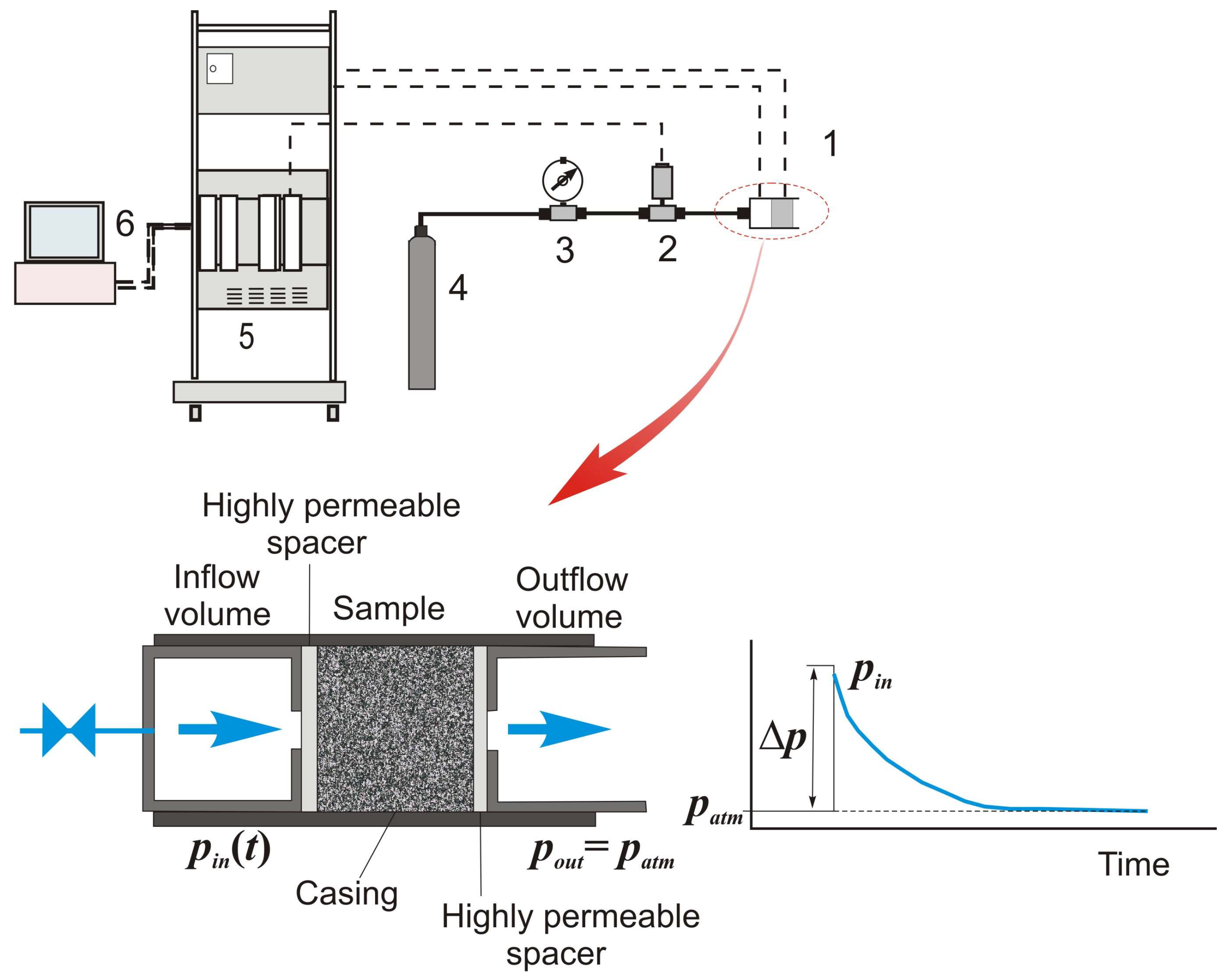
2.1.2. Experimental Apparatus

The experimental arrangement for permeability measurements is presented schematically in Figure 1. The sample of diameter up to 25 mm and height up to 21 mm is mounted into the experimental cell (1). Argon is drawn from the reservoir (4) through the capillaries, via the model gauge (3), and the circuit with a pressure transducer (2) to the upstream reservoir of the experimental cell connected with the inlet section of the sample. From the outlet section, argon flows out to the atmosphere.

Permeability measurements can be carried out using the steady state method and the pulse decay method. In the first case, a volume meter is used for measuring the flowing gas volume. With the pulse decay method, an electronic registration system connected to a PC (6) is used. This system allows recording pT-parameters during the experiment and, in particular, time dependencies of gas pressure in the upstream reservoir. The data obtained are processed using software developed on the base of the described technique.

2.2. Anisotropic Permeability

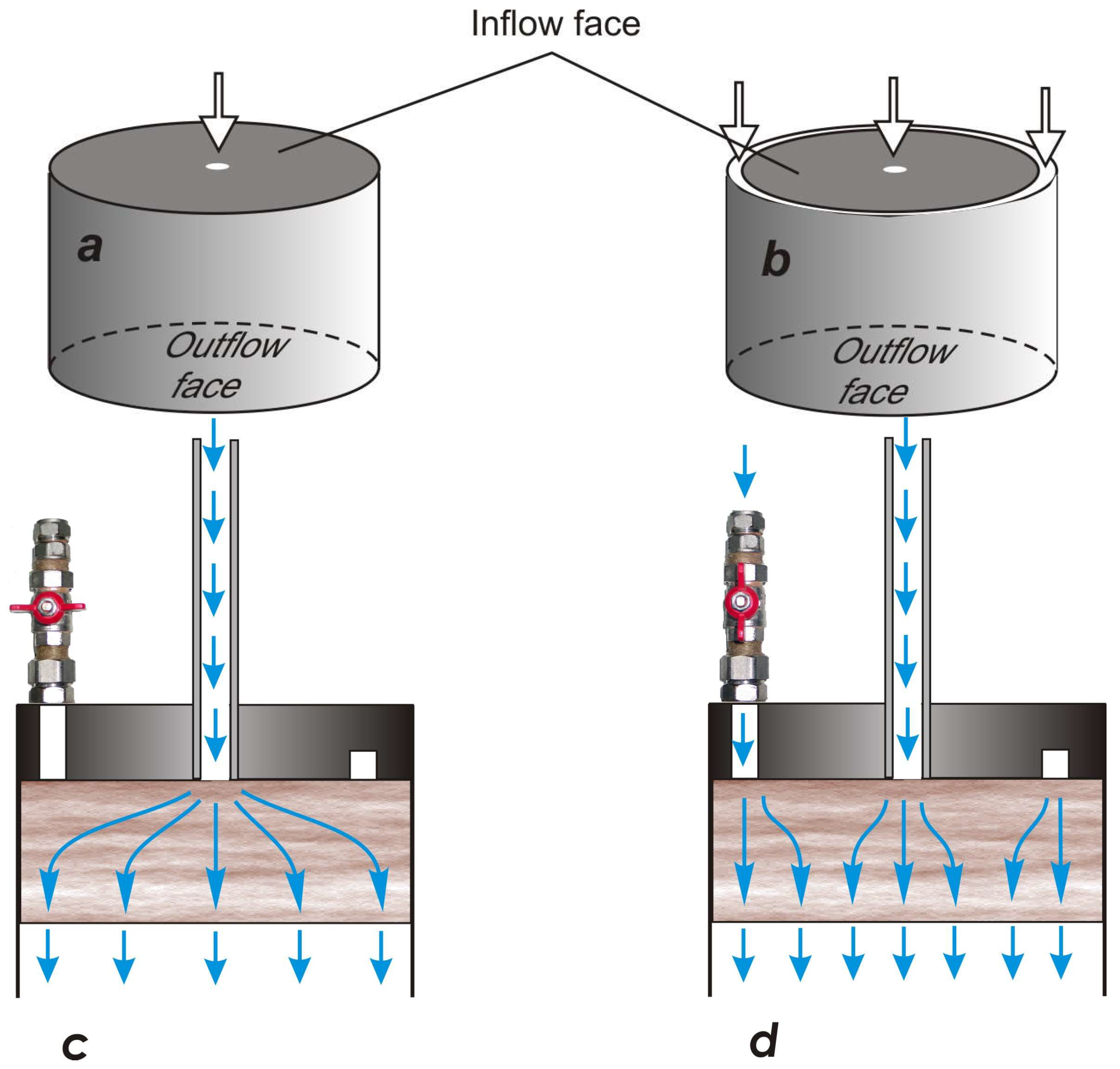
2.2.1. Experimental Apparatus

The measurement of isotropic permeability is usually carried out at homogeneous inflow and outflow of the fluid. This is implemented through the establishment of uniform distributions of the pressure in the inflow and outflow cross-sections of the rock sample. Streamlines of the fluid take the form of segments of straight lines in this case. Let us now consider the flow of the fluid through a sample of a rock with a layered anisotropy. The sample has the form of a cylinder with an axis normal to rock stratification. It follows from Darcy’s law that the fluid streamlines are also segments of straight lines at the uniform inflow and outflow of the fluid. However, if the inflow is not uniform, the streamlines become curvilinear, and the curvature of the lines depends on the anisotropy of the sample permeability. Let us consider a cylindrical sample of a layered rock with the impermeable casing of the side surface. The permeability of the sample is determined with the use of two operation modes, as is shown in Figure 2a,b.

The fluid flows into the sample at the first operation mode only through a circle of a small diameter in the inflow face (Figure 2a). The residual surface of the inflow face is impermeable to the fluid. The inflow of the fluid at the second operation mode is carried out through the same circle as through a narrow coaxial domain at the periphery of the inflow face (Figure 2b). The influence of anisotropy on the characteristics of the flow is different in these two cases (Figure 2c,d). Therefore, it seems to be possible to determine both longitudinal and transverse components of the permeability from a comparison of the characteristics of the flow at these two operation modes. For substantiation of this assumption, we consider the flow of a gas through a cylindrical sample of a layered rock.

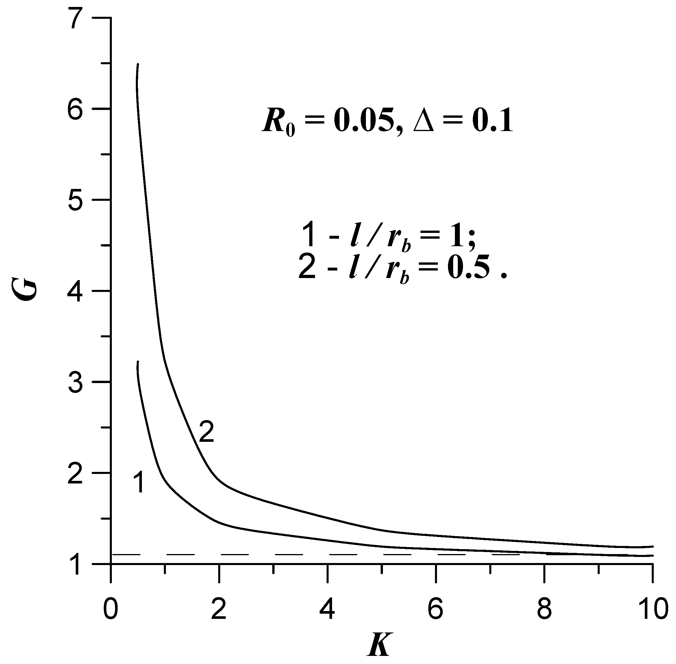
2.2.2. Theoretical Model

The axis of the sample is normal to the rock stratification. Considering the Klinkenberg effect, we can write expressions for the permeability components in the following forms

$$k_l=k_l^0\left(1+\frac{b}{p}\right),\hspace{1em}{k}_t=k_t^0\left(1+\frac{b}{p}\right)$$

where $k_{l,\hspace{0.33em}}{k}_t$ are the longitudinal and transverse components of the permeability, respectively; $k_l^0,\hspace{0.33em}{k}_t^0$ are the longitudinal and transverse components for the liquid.

Gases, which are used as fluids in the permeability measurements, can be considered as ideal ones at moderate temperatures. The process of the steady state flow of the gas through the sample is then governed by the non-linear Equation:

$$k_l^0\frac{\partial }{\partial z}\left[\left(p+b\right)\frac{\partial p}{\partial z}\right]+\frac{k_t^0}{r}\frac{\partial }{\partial r}\left[r\left(p+b\right)\frac{\partial p}{\partial r}\right]=0$$

(16)

where $r,z$ are cylindrical coordinates.

The solution of Equation (16) at corresponding boundary conditions gives a distribution of the gas pressure in the sample $p(r,z)$, and we can determine a mass of the gas which flows through the inflow face of the sample per unit time

$$w=\frac{2\pi k_l^0{\rho }_0}{\mu }\left(1+\frac{b}{p_0}\right){\displaystyle \underset{0}{\overset{r_b}{\int }}{\left.\frac{\partial p}{\partial z}\right|}_{z=0}r\hspace{0.17em}dr}$$

where $p_0$ is the pressure at the outflow face of the sample (at $z=0$); ${\rho }_0$ is the density of the gas at the outflow face; $r_b$ is the radius of the cylindrical sample; and $w$ is the bulk flow of the gas.

We denote $w_1$ and $w_2$ values of the bulk flow at the operation modes 1 and 2, respectively. Let us introduce a parameter of a relative bulk flow $G=w_2/w_1$ and a parameter of the anisotropy $K=k_t^0/k_l^0$.

The more pronounced the dependence $G(K)$, the more explicitly permits the comparison of the bulk flows of the gas at the first and the second operation modes to judge an extent of the permeability anisotropy. The bulk flow values are determined by the finite element method based on the Galerkin’s technique [30]. The calculations show that $G(K)$ is a monotonously decreasing function, and $G\to 1$ at $K\to \infty$ (Figure 3).

Hence, an accuracy of $K$ determination from the dependence $G(K)$ decreases at $G\cong$ 1. The more G differs from 1, the higher the accuracy of the $K$ determination. $K$ depends on a ratio of the sample dimensions $l/r_b$ where $l$ is the sample height. If $K\le 10$ and $l/r_b$ = 0.5, $G-1\ge 0.2$, i.e., the accuracy of the proposed technique of anisotropic permeability determination is sufficient at $l/r_b$ = 0.5 up to $K=10$.

3. Results and Discussion

Isotropic Permeability

The results of permeability measurements carried out on 7 samples of the different rocks: porphyrite (Porph-1, 2, 3, 4), basalt (B-1), and sandstone (Sand-1, 2) are presented in

Table 1. Permeability measurements results.

Sample	$\mathit{\phi }$	$\mathit{\delta }{\mathit{k}}_{\mathit{w}}/{\mathit{k}}_{\mathit{w}}$	${\mathit{k}}_{\mathit{w}}, {\mathbf{m}}^2$		$\mathit{b}$, Mpa		kw(Kl)	$1-{\mathit{k}}_{\mathit{w}}^{(\mathit{K}\mathit{l})}/{\mathit{k}}_{\mathit{w}}^{(\mathit{n}\mathit{u}\mathit{m})}$
			${\mathit{k}}_{\mathit{w}}^{(\mathit{a}\mathit{n})}$	${\mathit{k}}_{\mathit{w}}^{(\mathit{n}\mathit{u}\mathit{m})}$	${\mathit{b}}^{(\mathit{a}\mathit{n})}$	${\mathit{b}}^{(\mathit{n}\mathit{u}\mathit{m})}$
Porf-1	0.0021	0.154	2.48 × 10−20	2.427 × 10−20	2.499	2.568	3.8 × 10−20	−0.541
Porf-2	0.0026	0.376	6.974 × 10−20	6.764 × 10−20	1.757	1.835	8.5 × 10−20	−0.257
Porf-3	0.0027	0.286	3.011 × 10−20	2.897 × 10−20	1.266	1.361	2.6 × 10−20	0.103
Porf-4	0.0033	0.117	1.111 × 10−19	1.069 × 10−19	1.182	1.259	1.1 × 10−19	−0.029
Sand-1	0.1370	0.155	2.707 × 10−15	2.543 × 10−15	0.4501	0.5088	2.0 × 10−15	0.214
Sand-2	0.0998	0.118	1.687 × 10−15	1.616 × 10−15	0.6529	0.7014	1.6 × 10−15	0.010
B-1	0.1990	0.191	1.009 × 10−16	9.417 × 10−17	1.007	1.117	1.0 × 10−16	−0.062

.

The $k_w^{(an)}$ and $b^{(an)}$ values are determined by the analytical solution (11) (without regard to the damping influence of gas in the sample pore space and dependence of gas viscosity on pressure). The $k_w^{(num)}$ and $b^{(num)}$ values are determined using the numerical solution of the filtration problem (5)–(9) in the general formulation.

Since the values of $k_w^{(num)}$ and $b^{(num)}$ are obtained using a generalized model of the process, they appear to be more valid. However, it could be noted that the differences between the values of $k_w^{(num)}$ and $k_w^{(an)}$ are not higher than 7% of $k_w^{(num)}$. The value of $k_w^{(an)}$ is evaluated using an analytical approximation of the process under the assumption that the pore volume of a sample is negligibly small, and the damping influence of gas inherent in a sample can be ignored. Hence, as in CPDT, it follows that the differences between $k_w^{(num)}$ and $k_w^{(an)}$ shall be as greater as the higher the sample porosity value ($\phi$) becomes (see Figure 4). As it was obtained in refs. [9,10,11], this difference in CPDT did not exceed 10% $\phi$ < 0.25, which is in good agreement with our results presented in Figure 2.

Since the ratio of the effective sample pore volume to the reservoir volume did not exceed 0.04 in our experiments, the satisfactory agreement between values of $k_w^{(num)}$ and $k_w^{(an)}$ corresponds to the results obtained by Trimmer [11].

For a validity assessment of the results obtained, the value of $k_w^{(Kl)}$ for all samples studied has been determined using the classical Klinkenberg method [23]. The $k_w^{(Kl)}$ values have been compared with the values of $k_w^{(num)}$ determined using the technique described above. Differences between these values for all samples studied (see the table) except Porph-1 did not exceed 26%. However, as it could be seen from Figure 5, the values of $p_{in}(t_i)$ calculated at $k_w^{(num)}$ and $b^{(num)}$ for Porph-1 are in good agreement with measured ones, and a sufficiently rigid estimation by formula (15) shows that the accuracy of $k_w^{(num)}$ determination is quite satisfactory (see Table 1).

This permits us to suppose that the discrepancy between $k_w^{(Kl)}$ and $k_w^{(num)}$ for Porph-1 arises from the fact that the gas pressure range in the experiments using the Klinkenberg method was not sufficient for the determination of $k_w^{(Kl)}$ with a proper accuracy.

An example of the technique application for measurement of the anisotropic permeability of the dacite sample from the uranium ore deposit Streltsovka (Transbaikalia, Russia) is presented in Figure 6. The obtained values of the anisotropic permeability components are $k_l^0$ = 0.152 × 10⁻¹⁸ m², $k_t^0$ = 0.658 × 10⁻¹⁷ m².

4. Conclusions

The laboratory measurements of rock permeability are often carried out using gas as a flowing medium. This is dictated by the necessity to obtain essentially higher filtration rates than in the case when liquid is used and, as a result, to enhance the accuracy of measurements and reduce their duration.

The pulse decay method is widely used in such experiments. The procedure of data processing used in this method in its ‘traditional’ way is valid only for those experiments in which a ratio between gas pressures at the inlet and outlet of the sample is approximately equal to 1. Therewith, to determine the permeability of the sample in relation to water, it is necessary to carry out a series of experiments at different average gas pressures. As a result, the total duration of measurements increases. Moreover, the errors introduced by every experiment can accumulate during final data processing, and hence, the accuracy of the results obtained can dramatically be reduced.

Hereby a modification of the pulse decay method has been developed which permits: (i) to determine simultaneously the permeability value of a rock sample in relation to fluid and the Klinkenberg constant from data of a single experiment; (ii) to reduce experiment duration; (iii) to simplify the recording of p_in(t) dependence and to improve its accuracy at the cost of an increase in pressure step value (Δp).

For the method of measurements of rock permeability, proposed special equipment and software have been developed and tested using rocks with different reservoir properties. Analysis of data obtained and comparison with ones derived from the same samples by the Klinkenberg method shows satisfactory accuracy and higher efficiency of the modified pulse decay technique.

The modified pulse technique proposed can be used as the basis for developing unified testing protocols for measurements of rock permeability.

References

1. Pek, A.A. On the Dynamic of Juvenile Solutions; Nauka: Moscow, Russia, 1968. [Google Scholar]
2. Malkovsky, V.I.; Pek, A.A.; Arseniev, P.L.; Topor, D.N. Modeling of convective heat and mass transport at fluids flow along fault zones. Izvestya RAN Phisika Zemli 1988, 12, 57–62. [Google Scholar]
3. Tutubalin, A.V.; Grichuk, D.V.; Malkovsky, V.I. A complex hydrodynamic model of a convective hydrothermal system. In Proceedings of the 8th International Symposium “Water-Rock Interaction-WRI-8”, Vladivostok, Russia, 15–19 August 1995; Balkema: Rotterdam, The Netherlands, 1995; pp. 763–766. [Google Scholar]
4. Malkovsky, V.I.; Pek, A.A.; Omelyanenko, B.I.; Drojko, E.G. Numerical simulation of thermocon-vective transport of radionuclides by groundwater from the well-type repository of high-level radioactive waste. Izvestya RAN Energ. 1994, 3, 113–122. [Google Scholar]
5. Kissin, I.G. Fluids in the Earth’s Crust, 2nd ed.; Nauka: Moscow, Russia, 2015; 328p. [Google Scholar]
6. Morrow, C.; Byerlee, J. Permeability of rock samples from Cajon Pass, California. J. Geophys. Res. 1988, 15, 1033–1036. [Google Scholar] [CrossRef]
7. Morrow, C.; Lockner, D. Permeability difference between surface-derived and deep drill hole core samples. J. Geophys. Res. 1994, 21, 2151–2154. [Google Scholar]
8. Brace, W.F.; Walsh, J.B.; Frangos, W.T. Permeability of granite under high pressure. J. Geophys. Res. 1968, 73, 2225–2236. [Google Scholar] [CrossRef]
9. Hsieh, P.A.; Tracy, J.V.; Neuzil, C.E.; Bredehoeft, J.D.; Silliman, S.E. A transient laboratory method for determining the hydraulic properties of tight rocks-I Theory. Int. J. Rock Mech. Min. Sci. Geomech. Abstr. 1981, 18, 245–252. [Google Scholar] [CrossRef]
10. Lin, W. Parametric analyses of the transient method of measuring permeability. J. Geophys. Res. 1982, 87, 1055–1060. [Google Scholar] [CrossRef]
11. Trimmer, D.B.; Bonner, H.C.; Duba, A. Effect of pressure and stress on water transport in intact and fractured gabbro and granite. J. Geophys. Res. 1980, 85, 7059–7071. [Google Scholar] [CrossRef]
12. Lin, C.; Pirie, G.; Trimmer, D.A. Low Permeability Rocks-Laboratory Measurements and 3-Dimensional Microstructural Analysis. J. Geophys. Res. 1986, 91, 2173–2181. [Google Scholar] [CrossRef]
13. Katsube, T.J.; Mudford, B.S.; Best, M.E. Petrophysical Characteristics of Shales from the Scotian Shelf. Geophysics 1991, 56, 1681–1689. [Google Scholar] [CrossRef]
14. Le Guen, C.; Deveughele, M.; Billiotte, J.; Brulhet, J. Gas-permeability changes of rock-salt subjected to thermomechanical stresses. Q. J. Eng. Geol. 1993, 26, 327–334. [Google Scholar] [CrossRef]
15. Zeynalyandabily, E.M.; Rahman, S.S. Measurement of Permeability of Tight Rocks. Meas. Sci. Technol. 1995, 6, 1519–1527. [Google Scholar] [CrossRef]
16. Cao, C. Numerical interpretation of transient permeability test in tight rock. J. Rock Mech. Geotech. Eng. 2018, 10, 32–41. [Google Scholar] [CrossRef]
17. Zhao, Y.; Zhang, K.; Wang, C.; Bi, J. A large pressure pulse decay method to simultaneously measure permeability and compressibility of tight rocks. J. Nat. Gas Sci. Eng. 2022, 98, 104395. [Google Scholar] [CrossRef]
18. Wang, Y.; Tian Zh Nolte, S.; Krooss, B.M.; Wang, M. An improved straight-line method for permeability and porosity determination for tight reservoirs using pulse-decay measurements. J. Nat. Gas Sci. Eng. 2022, 105, 104708. [Google Scholar] [CrossRef]
19. Fischer, G.J.; Paterson, M.S. Permeability and storage capacity during deformation at elevated temperatures. In Fault Mechanics and Transport Properties of Rocks; Elsevier: St. Diego, CA, USA, 1992; pp. 187–211. [Google Scholar]
20. Zhang, S.; Paterson, M.S.; Cox, S.F. Porosity and permeability evolution during hot isostatic pressing of calcite aggregates. J. Geophys. Res. 1994, 99, 15741–15760. [Google Scholar] [CrossRef]
21. Sander, R.; Pan, Z.; Connell, L. Laboratory measurement of low permeability unconventional gas reservoir rocks: A review of experimental methods. J. Nat. Gas Sci. Eng. 2017, 37, 248–279. [Google Scholar] [CrossRef]
22. Zharikov, A.V.; Vitovtova, V.M.; Shmonov, V.M. Experimental study of permeability of Archean rocks from the Kola super deep drill hole. Geol. Rudn. Mestorojdeniy 1990, 32, 79–88. [Google Scholar]
23. Klinkenberg, L.J. The permeability of porous media to liquids and gases. In Drilling and Production Practice; API: New York, NY, USA, 1941; pp. 200–211. [Google Scholar]
24. Scott, D.S.; Dullien, F.A.L. The flow of rarefied gases. AIChE J. 1962, 15, 293–297. [Google Scholar] [CrossRef]
25. Zaraisky, G.P.; Balashov, V.N. Thermal decompaction of rocks. In Fluids in the Crust; Shmulovich, K.I., Yardley, B.W.D., Gonchar, G.G., Eds.; Springer: Dordrecht, The Netherlands, 1994. [Google Scholar] [CrossRef]
26. Lanczos, C. Applied Analysis; Dover Publications Inc.: New York, NY, USA, 1988; 539p. [Google Scholar]
27. Gill, P.h.E.; Murray, W.; Wright, M.H. Practical Optimization; SIAM: Philadelphia, PA, USA, 2019; 401p. [Google Scholar]
28. Roache, P.J. Computational Fluid Dynamics; Albuquerque: Hemrosa, CA, USA, 1976. [Google Scholar]
29. Zubarev, V.N.; Kozlov, A.D.; Kouznetsov, V.M. Thermophysical Properties of Gases Important in Techniques at High Temperature and Pressure; Energoatomizdat: Moscow, Russia, 1989. [Google Scholar]
30. Zienkiewicz, O.C.; Morgan, K. Finite Elements and Approximation; Dover Publications: Newburyport, MA, USA, 2013; 574p. [Google Scholar]
Figure 1. Schematic arrangement of the experimental setup for rock permeability study: 1—experimental cell, 2—transducer, 3—gauge, 4—argon reservoir, 5—registration and control unit, 6—PC. (Capillaries are shown by solid lines, electrical connections are shown by dashed lines).
Inventions 08 00014 g001
Figure 2. Operation modes of gas inflow in measurement of anisotropic permeability on a sample: (a) the first operation mode; (b) the second operation mode, directions of the gas inflow are shown with white arrows, parts in the inflow face where the gas flows into the sample are shown in white. Flow lines: (c) the first operation mode; (d) the second operation mode.
Inventions 08 00014 g002
Figure 3. Dependence between the relative bulk flow and the permeability anisotropy at different ratios of sample dimensions.
Inventions 08 00014 g003
Figure 4. Dependence of the difference between numerical and analytical solutions (kw(num)- kw(an)) on sample porosity (φ).
Inventions 08 00014 g004
Figure 5. Results of permeability calculation for the sample Porf-1.
Inventions 08 00014 g005
Figure 6. Results of anisotropic permeability calculation for dacite. The first operation mode: (1) measured pressure in the inflow volume; (2) calculated pressure; The second operation mode: (3) measured pressure in the inflow volume; (4) calculated pressure.
Inventions 08 00014 g006