Development of a Method for Improving the Energy Efficiency of Oil Production with an Electrical Submersible Pump

Abstract

Most of the operating oil fields are in the late stages of development, in which special attention is paid to the oil production energy efficiency. In accordance with the trend toward the digitalization of technical processes, intelligent control stations for production wells are currently being developed, one of the main tasks of which is to maintain the equipment operation in an optimal mode. This work aims to develop a methodology for selecting an energy-efficient well operation mode by choosing the methods for controlling an electrical submersible pump. To solve this problem, a mathematical apparatus for calculating power consumption is presented, which considers the well pressure curve, while taking into account its degradation when pumping reservoir fluids, the fluids’ properties, the supply of demulsifier, and the equipment’s operating parameters. Based on the simulation results, it is revealed that the optimal method for controlling electrical submersible pump installations is a combination of frequency control and choke control. The reduction in specific power consumption with the combined control relative to the use of separate control types is up to 7.30%, and in the case of additional use of a demulsifier, it is up to 12.01%. The developed algorithms can be implemented based on programmable logic controllers of intelligent control stations.

1. Introduction

Currently, most oil and gas fields have reached the late stages of development [1]. Oil production at such fields is characterized by a constant or declining dynamics of oil production, an increase in the water cut of well production, and an increase in the number of factors that complicate the processes of oil production and transportation [2]. The number of such deposits in the world is steadily growing, and the main task of the subsoil user is to optimize the costs of ensuring their uninterrupted operation [3,4]. Let us consider the energy consumption structure of the mature Volga-Ural Petroleum and Gas Province oil field, which is given in [5] and presented in Figure 1.

As can be seen from this figure, the largest share in the structure of energy consumption of a mature oil field is occupied by mechanized oil production. On the territory of Volga-Ural Petroleum and Gas Province, the majority of wells (over 99%) are operated by a mechanized method. Moreover, one of the main methods of production is the use of an electrical submersible pump (ESP). As a result, the paper considers an urgent task to be optimizing the power consumption of the ESP and the efficiency of its operation. The main methods for optimizing the operation of the ESP are the correct selection of the pump by using the methods of nodal analysis, the introduction of new technologies and equipment, the optimization of the ESP’s operation mode, the introduction of control systems, and the automation of the production process and the fight against complications [6,7,8].

Considering the causes of complications in the process of oil production and transportation, it should be noted that the most common causes are the formation of solid organic deposits and the formation of high-viscosity emulsions during the passage of oil through the ESP [9,10]. In the case of the formation of organic deposits, their control involves reducing the rate of their formation or regular removal. It is important to note that with the correct choice of the method of control, it is possible to minimize the impact of this complication on the work of the ESP. The formation of high-viscosity emulsions (HVE) consists of an intensive mixing of oil and water, during which the latter is dispersed into tiny particles and creates an emulsion with a viscosity significantly higher than that of oil and water [11]. In the presence of a large number of organic surfactants in oil, a high viscosity of oil, and similar densities of oil and water, the emulsion can become stable, i.e., retain its properties for a long time [12]. The formation of HVE leads to an instant degradation of the pump head characteristic, an increase in pressure in the system, and a decrease in the efficiency of oil production [13,14]. The main method of combating the formation of HVE is dosing a chemical reagent, or a demulsifier. Its role is to permeate into the interfacial film stabilized by the surfactants and substitute the surfactants to break the interfacial film, reduce the stability of the emulsion, and lead to oil separation from water [15,16]. The destruction of the emulsion during the production and transportation of oil is a long process; however, when dosing the emulsion by introducing surfactants into the flow, it is possible to achieve a decrease in the viscosity of the emulsion. The use of these reagents is also considered as a method of optimizing the operation of HVE wells.

The operation of the ESP is provided by the surface equipment, which is the control station. The basic functionality of this equipment is turning the pump on and off; the pump is turned off when the measured parameter exceeds the set limits and the ability to start according to a schedule [17,18]. However, the modern oil industry is characterized by a strong trend toward the digitalization of all technological processes, including ESP management [19,20]. As part of this trend, intelligent control stations (ICS) are being developed and applied [21,22,23]. Their main advantage is the use of elements of artificial intelligence and machine learning. Thus, the list of modern ICS functions includes automatic optimization of ESP operation, reduction of energy consumption by selecting the most optimal operating modes, analysis of well operation data, and minimization of emergency situations [24,25,26]. An important task in the operation of ICS is the correct choice of the way to control the operation of the well.

At present, in the real oil field, the regulation of the parameters of production wells is carried out without accurate technological calculations. Thus, to regulate the well operation parameters, a periodic operation mode can be used, in which the submersible motor starts and stops at a frequency of up to several times a day. At the same time, the choice of a control method is often based on the experience of operating a well, without taking into account the energy efficiency of a particular method. Another fairly common method for controlling well productivity is a choke, the principle of which is based on creating a pressure drop by installing a choke with a diameter smaller than the diameter of the tubing in the flow line [27], as well as frequency control, which is based on a change in pump performance due to a change in the submersible motor rotation speed [28]. At the same time, it should be considered that a decrease in the choke diameter increases pressure losses, and a change in the speed of the pump rotation leads to both a change in the well operation parameters and a change in the pump efficiency due to a change in its operating point [29]. The simultaneous changes in these parameters can have a significant impact on the oil-producing energy efficiency and they must be considered when forming a map of energy-efficient modes of the field operation. The works in [30,31] present methods for optimizing technological processes based on the Model Predictive Control (MPC) approach. In particular, they describe the application of this algorithm to maintain pressure at the ESP intake with minimal energy consumption, which allows the optimization of a generated fluid rise model. However, in these works, simplified equations are used to model the oil production process and the assessment of electricity consumption does not take into account a number of components. In this regard, it is important to develop a methodology for calculating both the optimal parameters of the well equipment and the operation parameters of this equipment to select an energy-efficient operating mode for electrical submersible pump installations.

The rest of this paper is organized as follows: Section 2 describes the methods for calculating the well performance and for measuring the rheological properties of the well product, the power consumption of the electrical submersible pump unit, and the effect of fluid viscosity on the head performance. In Section 3, an example of applying the methodology to three oil producing wells is considered, and the parameters of their operation, the simulated operating modes, and the results of evaluating the energy efficiency of various well control methods are indicated. This paper ends with a discussion (Section 4), where the results of applying the methodology are noted, the results of estimating its error are described, and a conclusion is made about the practical application of this methodology.

2. Materials and Methods

2.1. Calculation of Well Characteristics

The well-known correlation proposed by Hagedorn and Brown [32] was used to determine the well characteristic (Vertical Lift Performance). The core of this method is a correlation for the liquid holdup [33].

The influence of the choke is considered by determining the pressure loss in it according to the method described in the work [27]. The following is an algorithm for calculating the pressure loss at the nozzle. This algorithm includes two formulas: the choke flow coefficient and the flow rate through the choke for a given set of parameters.

$${\mathrm{Q}}_{\mathrm{ESP}}=0.1683\cdot {\mathrm{C}}_{\mathrm{D}}\cdot \mathrm{A}\cdot \sqrt{\frac{\mathsf{\Delta }\mathrm{P}}{{\mathsf{\rho }}_{\mathrm{fl}}}},$$

(1)

$${\mathrm{C}}_{\mathrm{D}}=\frac{{\mathrm{d}}_{\mathrm{ch}}}{{\mathrm{d}}_{\mathrm{t}}}+\frac{0.3167}{{\left(\frac{{\mathrm{d}}_{\mathrm{ch}}}{{\mathrm{d}}_{\mathrm{t}}}\right)}^{0.6}}+0.025\left(\ln \left({\mathrm{N}}_{\mathrm{Re}}\right)-4\right)$$

(2)

where Q_ESP is the ESP flow rate (it is equal to the fluid flow through the choke), in m³/day; C_D is the choke flow coefficient, in units; A is the choke area, in m²; ΔP is the differential pressure, in MPa; ρ_fl is the lifted fluid density, in kg/m³; d_ch is the choke diameter, in m; d_t is the tubing diameter, in m; and N_Re is the Reynolds number, in units.

The choke flow coefficient is determined for nozzle-type chokes in [34]. When determining the pressure loss, this value is expressed as in the second formula. After determining the pressure loss in the choke, this value is added to the wellhead pressure, while taking into account the Hagedorn and Brown correlation as the required head of the oil gathering system.

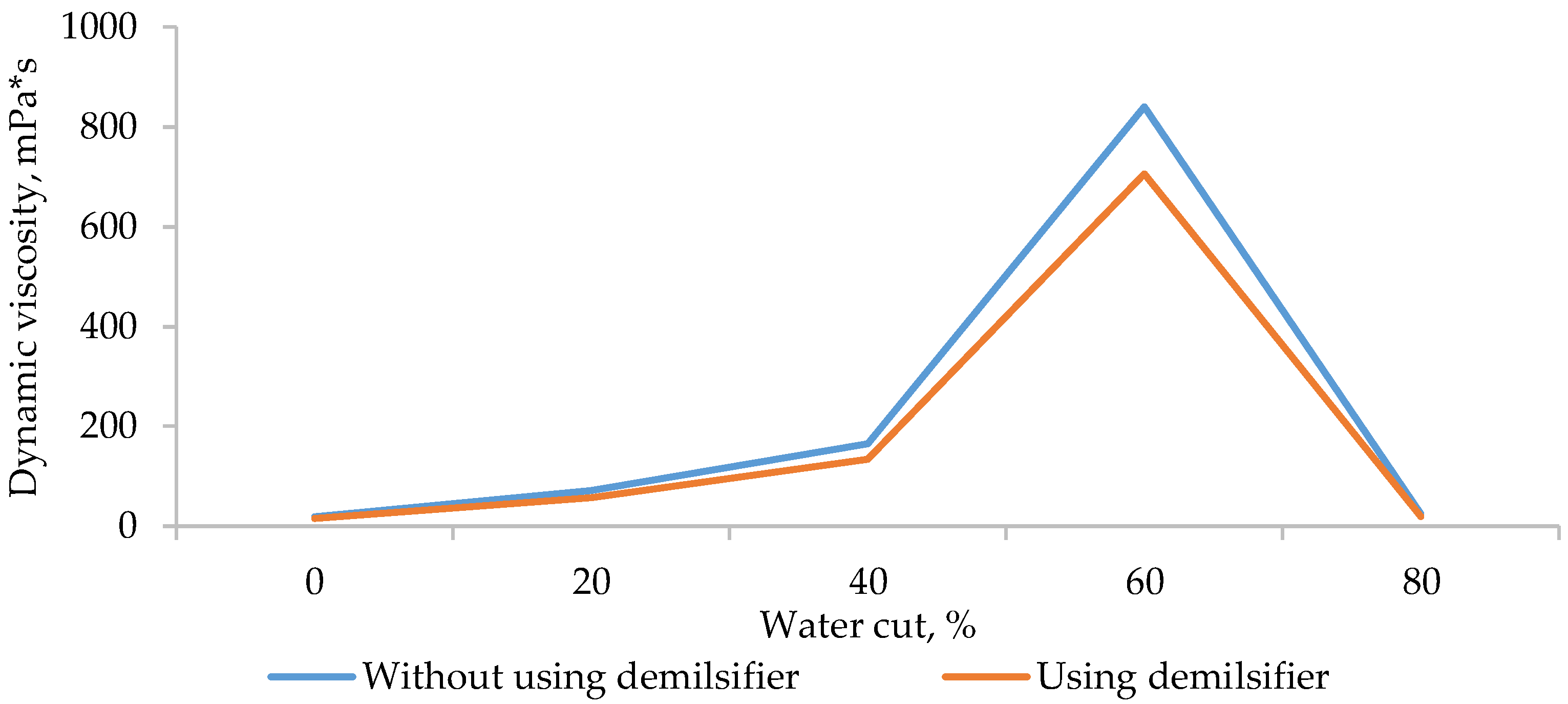
2.2. Determination of the Effect of Demulsifier Feed on HVE Viscosity

For this research, the oil and water samples were taken from the wells under consideration. To study the properties of the emulsion, oil and water were mixed in the required proportion at a speed corresponding to the ESP rotation speed for a time equal to the oil flow time through the ESP. After creating the emulsion, its dynamic viscosity was determined on a rotational viscometer Rheotest RN-4.1. In the case of using a demulsifier, it was supplied at the moment at the beginning of phase mixing. As part of the study, the viscosity of the emulsion was determined with and without a demulsifier in the range of water cut from 0 to 80%.

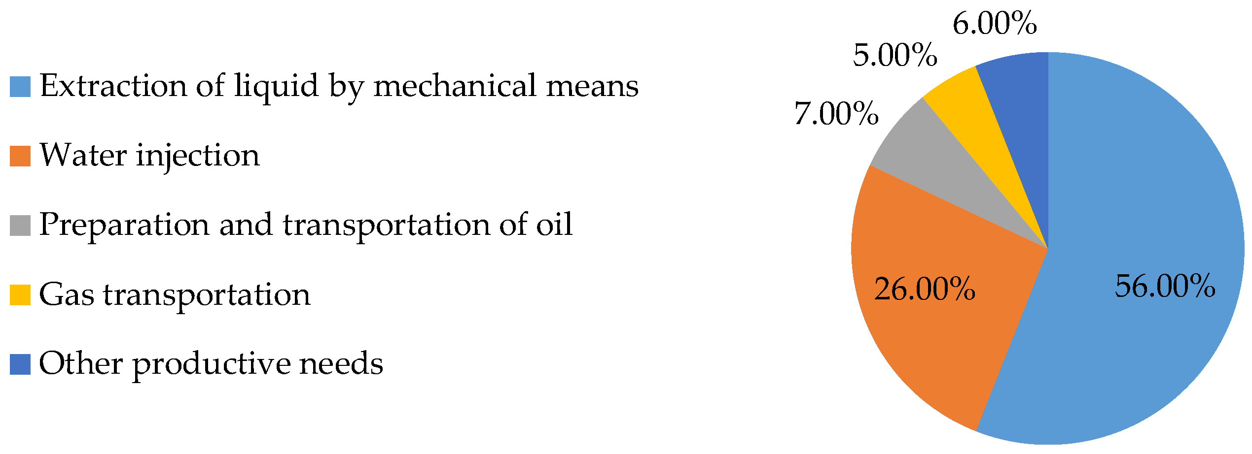
2.3. Calculation of the Power Consumption of an Electrical Submersible Pump Installation

The total electrical power consumed by an electric submersible pump installation (ESPI) is determined by the net power consumed by the motor and the sum of power losses in all other elements of the ESPI, in kW [35]:

$${\mathrm{P}}_{\mathrm{ESPI}}{=\mathrm{P}}_{\mathrm{SEM}}+{\mathsf{\Delta }\mathrm{P}}_{\mathrm{CL}}+{\mathsf{\Delta }\mathrm{P}}_{\mathrm{T}}+{\mathsf{\Delta }\mathrm{P}}_{\mathrm{CS}}.$$

(3)

It should be noted that chaotic oscillations can occur in real electrical circuits, which leads to a difference between the calculations results based on the model and the measurement data based on real objects [36]. However, when calculating the power consumption of the ESPI, due to the complex installation design, it is not possible to decompose one into simple circuits and estimate the value of chaotic oscillations. In this regard, the calculation of these oscillations in this work is not performed.

2.3.1. Electrical Submersible Pump

The pump’s mechanical power is calculated as follows, in kW:

$${\mathrm{P}}_{\mathrm{pump}}=\frac{{\mathsf{\rho }}_{\mathrm{fl}}\cdot \mathrm{g}\cdot \left(\frac{{\mathrm{P}}_{\mathrm{WH}}}{{\mathsf{\rho }}_{\mathrm{fl}}\cdot \mathrm{g}}{+\mathrm{H}}_{\mathrm{dyn}}\right)\cdot {\mathrm{Q}}_{\mathrm{ESP}}}{{\mathsf{\eta }}_{\mathrm{pump}}\cdot {\mathrm{K}}_{\mathsf{\eta }\mathsf{\nu }}\cdot 86400\cdot {10}^3},$$

(4)

where P_WH is the wellhead pressure, in Pa; H_dyn is the dynamic level, in m; g is the gravity acceleration, in m²/s; η_pump is the pump efficiency at the operation point, in p.u.; and K_ην is the coefficient considering the change in pump efficiency when operating on viscous liquids, in p. u.

The mathematical calculation of the pump efficiency depends on the parameters of the pump head curves (PHC), which are parameters of the electrical and technological mode, in p.u.:

$${\mathsf{\eta }}_{\mathrm{pump}}={\displaystyle \sum _{\mathrm{i}=0}^4{\mathrm{a}}_{\mathrm{i}}{\left(\frac{{\mathrm{f}}_{\mathrm{np}}}{\mathrm{f}}\right)}^{\mathrm{i}}\cdot {\left(\frac{{\mathrm{Q}}_{\mathrm{ESP}}}{{\mathrm{Q}}_{\max }}\right)}^{\mathrm{i}}},$$

(5)

where a_i is the polynomial weight coefficients, in units; f_np is the nameplate voltage frequency, in Hz; f is the voltage frequency, in Hz; Q_max is the theoretically possible maximum pump flow rate at a head equal to 0 m, in m³/day.

The polynomial coefficients of the ESP efficiency are determined by the pump passport curves.

The coefficient of change in the ESP efficiency when operating on viscous liquids is determined by the following formula, in p.u.:

$${\mathrm{K}}_{\mathsf{\eta }\mathsf{\nu }}=\frac{1}{1+0.4\left({\mathsf{\nu }-\mathsf{\nu }}_{\mathrm{w}}\right)},$$

(6)

where ν is the kinematic fluid viscosity, in sm²/s, and ν_w is the kinematic water viscosity, in sm²/s.

2.3.2. Submersible Electric Motor

The submersible electric motor (SEM) active power is determined by the following formula, in kW:

$${\mathrm{P}}_{\mathrm{SEM}}=\frac{{\mathrm{P}}_{\mathrm{pump}}}{{\mathsf{\eta }}_{\mathrm{SEM}}},$$

(7)

where η_SEM is the SEM efficiency at the current load factor value, in p.u.

The motor efficiency at various load factor values is determined based on the load curves provided by the manufacturer. To automate the calculations, the change in efficiency is described by a polynomial, in p.u.:

$${\mathsf{\eta }}_{\mathrm{SEM}}=\left(0.659\cdot {\mathrm{K}}_{\mathrm{L}}^4-0.367\cdot {\mathrm{K}}_{\mathrm{L}}^3-1.836\cdot {\mathrm{K}}_{\mathrm{L}}^2+2.288\cdot {\mathrm{K}}_{\mathrm{L}}+0.259\right)\cdot {\mathsf{\eta }}_{\mathrm{SEMnp}},$$

(8)

where η_SEMnp is the nameplate SEM efficiency, in p. u.

The SEM power losses are calculated as follows, in kW:

$$\mathrm{\Delta }{\mathrm{P}}_{\mathrm{SEM}}{=\mathrm{P}}_{\mathrm{SEM}}-{\mathrm{P}}_{\mathrm{pump}}.$$

(9)

The SEM load factor value is determined as follows, in p.u.:

$${\mathrm{K}}_{\mathrm{L}}=\frac{{\mathrm{P}}_{\mathrm{pump}}}{{\mathrm{P}}_{\mathrm{SEMnp}}}$$

(10)

where P_SEMnp is the SEM nameplate power, in kW.

The SEM current is determined as follows, in A:

$${\mathrm{I}}_{\mathrm{SEM}}=\frac{{\mathrm{P}}_{\mathrm{SEM}}}{\sqrt{3}\cdot {\mathrm{U}}_{\mathrm{SEMnp}}\cdot \frac{\mathrm{f}}{{\mathrm{f}}_{\mathrm{np}}}\cdot {\cos \mathsf{\phi }}_{\mathrm{SEM}}},$$

(11)

where U_SEMnp is the SEM nameplate voltage, in kV, and cos φ_SEM is the SEM power factor at the current load factor value, in p. u.

The SEM power factor value at various load factor values is determined based on the load curves provided by the manufacturer. To automate the calculations, the change in power factor is described by a polynomial, in p.u.:

$$\cos {\mathsf{\phi }}_{\mathrm{SEM}}=\left(-0.866\cdot {\mathrm{K}}_{\mathrm{L}}^2+1.964\cdot {\mathrm{K}}_{\mathrm{L}}+0.156\right)\cos {\mathsf{\phi }}_{\mathrm{SEMnp}},$$

(12)

where cos φ_SEMnp is the SEM nameplate power factor, in p. u.

2.3.3. Cable Line

The cable line parameters (CL) are calculated as follows, in Ohm:

$${\mathrm{r}}_{\mathrm{CL}}={\mathrm{r}}_0\cdot {\mathrm{l}}_{\mathrm{CL}}\cdot \left(1+\mathsf{\alpha }\left({\mathrm{T}}_{\mathrm{E}}-20\right)\right),$$

(13)

$${\mathrm{x}}_{\mathrm{CL}}={\mathrm{x}}_0\cdot {\mathrm{l}}_{\mathrm{CL}}\cdot \frac{\mathrm{f}}{50},$$

(14)

where r₀ and x₀ are the specific active and reactive resistance of cable line, in Ohm/km; l_CL is the cable line length, in km; α is the temperature coefficient of electrical resistance, in units (taken to be equal to 0.004 for a copper cable); and T_E is the environment’s temperature, in °C.

The environment’s temperature is determined by the formula in accordance with the average temperature increment in the lithosphere in the amount of 30 °C/km for the well as follows:

$${\mathrm{T}}_{\mathrm{E}}=15\cdot \left({\mathrm{H}}_{\mathrm{b}}{+\mathrm{H}}_{\mathrm{e}}\right){+\mathrm{T}}_0,$$

(15)

where T₀ is the soil temperature at the depth of non-freezing, which by default is equal to 5 °C. H_b and H_e are the depth at the beginning and at the end of the cable; in this case, the beginning depth is 0, and the end depth is equal to the cable length, in km.

The CL losses are determined as follows, in kW:

$${\mathsf{\Delta }\mathrm{P}}_{\mathrm{CL}}=3\cdot {\mathrm{I}}_{\mathrm{SEM}}{}^2\cdot {\mathrm{r}}_{\mathrm{CL}},$$

(16)

$${\mathsf{\Delta }\mathrm{Q}}_{\mathrm{CL}}=3\cdot {\mathrm{I}}_{\mathrm{SEM}}{}^2\cdot {\mathrm{x}}_{\mathrm{CL}}.$$

(17)

2.3.4. Transformer

The transformer (T) power losses are determined as follows, in kW:

$${\mathsf{\Delta }\mathrm{P}}_{\mathrm{T}}{=\mathsf{\Delta }\mathrm{P}}_{\mathrm{I}}+{\mathsf{\Delta }\mathrm{P}}_{\mathrm{L}},$$

(18)

$${\mathsf{\Delta }\mathrm{P}}_{\mathrm{I}}{=\mathsf{\Delta }\mathrm{P}}_{\mathrm{I}}\cdot {\left(\frac{\mathrm{f}}{50}\right)}^{1.3},$$

(19)

$${\mathsf{\Delta }\mathrm{P}}_{\mathrm{L}}{=\mathsf{\Delta }\mathrm{P}}_{\mathrm{CS}}\cdot {\left(\frac{\mathrm{S}}{{\mathrm{S}}_{\mathrm{Tnp}}}\right)}^2,$$

(20)

where ΔP_I is the passport value of the transformer idle losses, in kW; ΔP_I is the passport value of the transformer short-circuit losses, in kW; S is the transformer load corresponding to the calculated mode, in kVA; and S_Tnp is the transformer nameplate power, in kVA.

2.3.5. Control Station

The control station (CS) power losses are determined as follows, in p.u.:

$${\mathsf{\Delta }\mathrm{P}}_{\mathrm{CS}}=\left({\mathrm{P}}_{\mathrm{SEM}}{+\mathsf{\Delta }\mathrm{P}}_{\mathrm{CL}}{+\mathsf{\Delta }\mathrm{P}}_{\mathrm{T}}\right)\cdot \left(\frac{1}{{\mathsf{\eta }}_{\mathrm{CSnp}}}-1\right)$$

(21)

where η_CSnp is the nameplate CS efficiency, in p. u.

The specific power consumption is determined by the following formula, in kW∙h/m³:

$${\mathrm{W}}_{\mathrm{sp}}=\frac{{\mathrm{P}}_{\mathrm{ESPI}}\cdot \mathrm{T}}{{\mathrm{Q}}_{\mathrm{ESP}}},$$

(22)

where T is the considered well operation period, in h.

2.4. Optimal Frequency Value Calculation

Based on the theory of ESP, the minimum frequency value is calculated when the required pump flow with the minimum necessary head is provided. The order of calculation is shown below.

Based on the fact that the pump flow changes in proportion to the change in the pump shaft rotation speed, the minimum frequency of the supply voltage is calculated, below which the pump theoretically does not develop the required head (crossing of the pump head characteristic with the abscissa axis), in Hz:

$${\mathrm{f}}_{2\min }=\frac{{\mathrm{Q}}_2}{{\mathrm{Q}}_1}\cdot {\mathrm{f}}_1$$

(23)

where Q₁ is the pump flow, at a head equal to 0 at the main voltage frequency (the calculation should take into account the displacement of the pump head curve due to the influence of the viscosity of the produced fluid), in m³/day; Q₂ is the required pump rate, in m³/day; and f₁ is the main frequency of the supply voltage, in Hz.

The interval of possible frequency change is determined to control the flow rate at a given pressure, in Hz:

$${\mathsf{\Delta }\mathrm{f}=\mathrm{f}}_{\mathrm{cur}}{-\mathrm{f}}_{2\min },$$

(24)

where f_cur is the voltage frequency in the current mode, in Hz.

It is assumed that the change in the PHC has no restrictions, and the point of its intersection with the PHC is at the point with coordinates (Q₂; H₂). Then, the minimum allowable frequency is calculated, which will provide a given flow rate at the minimum allowable head:

$${\mathrm{f}}_2{=\mathrm{f}}_{2\min }+\mathsf{\Delta }\mathrm{f}\cdot \frac{{\mathrm{H}}_2}{{\mathrm{H}}_1}$$

(25)

where H₁ is the head corresponding to the current mode, in m, and H₂ is the required head, in m.

The CS frequency value is selected according to the rounding rules in accordance with the CS technical capabilities.

During frequency control, a check must be performed so that the wellhead pressure P_WH in the proposed mode is not lower than the line pressure (P_line) of the initial mode.

2.5. Influence of Fluid Viscosity on the Head Characteristic of a Pump

The PHC is described as follows, in m:

$${\mathrm{H}}_{\mathrm{ESP}}={\displaystyle \sum _{\mathrm{i}=0}^4{\mathrm{b}}_{\mathrm{i}}\cdot {\mathrm{Q}}_{\mathrm{ESP}}{}^{\mathrm{i}}}$$

(26)

where b_i is the polynomial weight coefficients, in units.

When describing the PHC, it should be considered that it can operate at a non-nominal frequency and adjust the characteristic while considering the similarity criteria.

It should also be considered that the passport PHC was built during the tests on water. When the pump is operating on viscous liquids, the head curve changes its appearance. These changes can be considered by the formulas [37] for the flow rate, in m³/day:

$${\mathrm{Q}}_{\mathrm{ESP}\mathsf{\nu }}{=\mathrm{Q}}_{\mathrm{ESP}\mathsf{\nu }}\cdot {\mathrm{K}}_{\mathrm{Q}\mathsf{\nu }},$$

(27)

and for the head, in m,

$${\mathrm{H}}_{\mathrm{ESP}\mathsf{\nu }}{=\mathrm{H}}_{\mathrm{ESP}\mathsf{\nu }}\cdot {\mathrm{K}}_{\mathrm{Q}\mathsf{\nu }}.$$

(28)

The pump rate change factor due to viscosity can be calculated as follows, in units:

$${\mathrm{K}}_{\mathrm{Q}\mathsf{\nu }}=1-\frac{4.95\cdot {\mathsf{\nu }}^{0.85}}{{\mathrm{Q}}_{\mathrm{o}\mathrm{w}}^{0.57}},$$

(29)

where Q_ow is the optimal ESP flow rate when using water, in m³/day.

The head change factor due to viscosity can be calculated as follows, in p.u.:

$${\mathrm{K}}_{\mathrm{H}\mathsf{\nu }}=1-\frac{1.07\cdot {\mathsf{\nu }}^{0.6}\cdot {\mathrm{q}}_{\mathrm{rel}}}{{\mathrm{Q}}_{\mathrm{o}\mathrm{w}}^{0.57}},$$

(30)

The relative flow rate at the pump intake at the corresponding operation point in the PHC when using water is defined as follows, p.u.:

$${\mathrm{q}}_{\mathrm{rel}}=\frac{{\mathrm{Q}}_{\mathrm{ESP}}\cdot \mathrm{B}\cdot {\mathrm{K}}_{\mathrm{Q}\mathsf{\nu }}}{{\mathrm{Q}}_{\mathrm{o}\mathrm{w}}},$$

(31)

where B is the fluid volume factor at the pump intake pressure, in p. u.

3. Results

3.1. Initial Data

Two wells from one of the Volga-Ural province oil fields were chosen as the objects of study. The parameters of the equipment installed on the wells are presented in

Table 1. Oil well equipment parameters.

Equipment	Parameter	Well
		1	2
Pump	Qnp, m3/day	80	80
	Qmax, m3/day	151.4	151.4
SEM	PSEMnp, kW	32	40
	USEMnp, V	1000	1300
	cos φSEMnp, p.u.	0.85	0.85
	ηSEMnp,%	84	91.5
	Inp,A	24.2	24
CL	r0, Ohm/km	2.1	2.1
	x0, Ohm/km	0.1	0.1
	L, km	1.39	1.33
T	ΔPI, kW	0.55	0.55
	ΔPSC, kW	2.6	2.6
	STnp, kVA	100	100
CS	ηCSnp, p.u.	0.97	0.97

.

The polynomial coefficients describing the pump head curve and the pump efficiency curve are presented in

Table 2. Polynomial coefficients for describing pump characteristics.

Parameter	Value
i	4	3	2	1	0
ηpump	0.000104	0.90676	0.14863	0.14755	−1.2593
PHC	3.02E-06	−0.00124	0.07774	−1.14269	1132.1

.

3.2. Determination of the Effectiveness of the Use of Demulsifiers

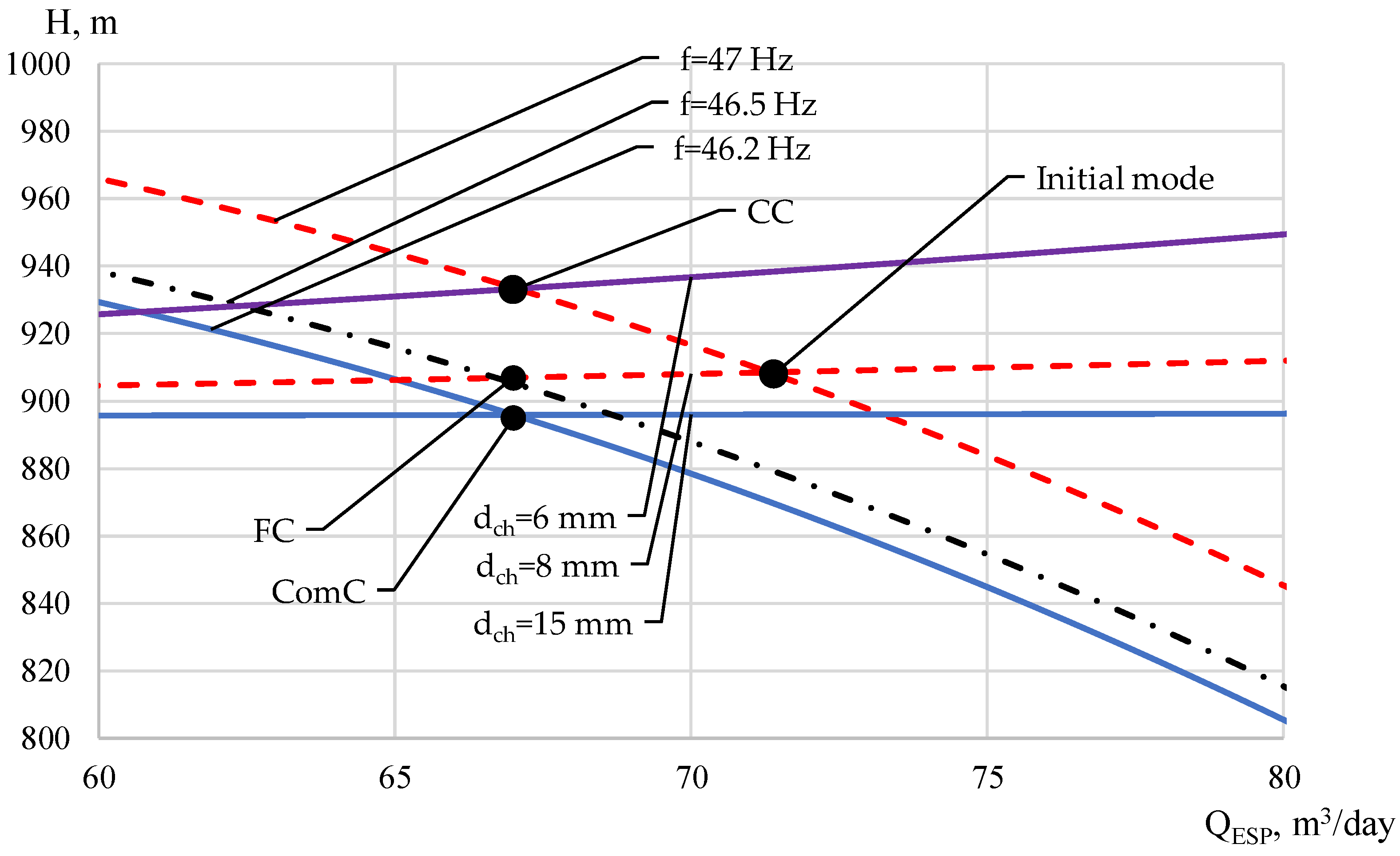
In the framework of this work, an industrially used modified nonionic surfactant was used as a demulsifier. As a result of the research, two oil demulsification curves are obtained, as shown in Figure 2.

As can be seen from the graphs obtained, the oil viscosity slightly decreases when a demulsifier is added to the ESP intake. This can lead to an increase in the efficiency of its operation and a decrease in pressure losses due to friction.

3.3. Modeling Modes

Since the technological mode of an oil field production well is planned for a day, the average daily values of the technological process parameters are used to calculate the power consumption and energy efficiency.

To assess the effectiveness of the control methods, the following application was considered:

• Initial mode;
• Choke control (CC);
• Frequency control (FC);
• Combined control (choke control and frequency control) (ComC).

For each of the control methods, except for the initial one, two options were considered:

• Without using a demulsifier (wUD);
• Without using a demulsifier (UD).

The boundary on the FC depth was that the wellhead pressure was not lower than the linear pressure in the initial mode.

The calculation of specific power consumption in the initial mode was performed to assess the model’s accuracy. The model accuracy was assessed through the relative error of calculations and the instrumental measurements on the objects under consideration.

To assess the effectiveness of the mode’s control methods, the situation of transferring the well to a lower flow rate was considered.

All parameters used in the calculation are presented in

Table 3. Calculation parameters.

Mode	Parameter	Well
		1	2
Constant parameters	B, p.u.	1.06	1.06
	ρfl, kg/m3	923	923
	Hdyn, m	915	827
	dt, mm	62	62
Initial mode	QESP, m3/day	71.3	74.4
	Pline, MPa	1.35	0.95
	PWH, MPa	1.5	1.1
	f, Hz	47	50
	dch, mm	8	8
Demulsifier	Without using demulsifier, Pa∙s	0.0711	0.0711
	Using demulsifier, Pa∙s	0.0569	0.0569
Choke control	QESP, m3/day	67	70
	PWH, MPa	1.76	1.25
	f, Hz	47	50
	dch, mm	6	6
Frequency control	QESP, m3/day	67	70
	PWH, MPa	1.46	1.08
	f, Hz	46.4	49.5
	dch, mm	8	8
Combined control	QESP, m3/day	67	70
	PWH, MPa	1.36	0.96
	f, Hz	46.2	49.3
	dch, mm	15	15

.

The model accuracy estimation is presented in

Table 4. Model accuracy estimation.

Parameter	Well
	1	2
Wsp (calculation), kW∙h/m3	11.03	8.16
Wsp (measurement), kW∙h/m3	10.77	8.33
Error, %	−2.39	2.03

.

The main equipment operation energy parameters corresponding to the calculated modes are presented in

Table 5. Energy parameters of the equipment operation.

Parameter	CC wUD	CC UD	FC wUD	FC UD	ComC wUD	ComC UD
PWH, MPa	1.76/1.25	1.76/1.25	1.46/1.08	1.46/1.08	1.36/0.96	1.36/0.96
Kην, p.u.	0.767/0.767	0.805/0.805	0.767/0.767	0.805/0.805	0.767/0.767	0.805/0.805
ηpump, p.u.	0.337/0.418	0.353/0.438	0.341/0.422	0.357/0.443	0.342/0.424	0.359/0.445
Ppump, kW	23.15/16.95	22.06/16.15	22.18/16.46	21.17/15.69	21.84/16.16	20.81/15.4
ηESM, p.u.	0.847/0.793	0.847/0.782	0.847/0.787	0.846/0.775	0.846/0.782	0.845/0.77
IESM, A	20/14.3	19.1/14	19.5/14.2	18.6/14	19.3/14.2	18.4/14
ΔPSEM, kW	4.18/4.41	4/4.5	4.02/4.46	3.86/4.56	3.96/4.5	3.81/4.6
ΔPCL, kW	3.82/1.84	3.47/1.77	3.6/1.84	3.28/1.77	3.53/1.82	3.21/1.76
ΔPT, kW	0.86/0.75	0.83/0.73	0.82/0.73	0.79/0.72	0.81/0.72	0.78/0.71
ΔPCS, kW	0.96/0.72	0.91/0.69	0.92/0.7	0.87/0.68	0.9/0.7	0.86/0.67
PESPI, kW	32.97/24.67	31.27/23.85	31.54/24.2	29.99/23.42	31.05/23.91	29.47/23.15

. The data before the “/” sign correspond to well № 1, and the data after the sign correspond to well № 2.

The results of the specific power consumption calculations for different control methods are presented in

Table 6. The calculation results of specific power consumption with different control methods.

Use of a Demulsifier	Wsp, kW∙h/m3
	CC	FC	ComC
	Well 1
wUD	11.81	11.30	11.12
UD	11.20	10.74	10.56
	Well 2
wUD	8.46	8.30	8.20
UD	8.18	8.03	7.94

.

The effectiveness evaluation of the control method application is presented in

Table 7. Comparison of energy efficiency of well control methods.

	CC wUD	CC UD	FC wUD	FC UD	ComC wUD	ComC UD
CC wUD	0/0	5.17/3.34	4.34/1.92	9.05/5.09	5.83/3.11	10.61/6.17
CC UD	-	0/0	−0.87/−1.47	4.1/1.81	0.7/−0.24	5.74/2.93
FC wUD	-	-	0/0	4.93/3.23	1.56/1.21	6.56/4.34
FC UD	-	-	-	0/0	−3.54/−2.08	1.72/1.14
ComC wUD	-	-	-	-	0/0	5.08/3.16
ComC UD	-	-	-	-	-	0/0

. The data before the “/” sign correspond to well № 1, and the data after the sign correspond to well № 2. The data in the cells correspond to the ratio of the specific power consumption of the mode indicated in the left column cell to the same indicator of the mode indicated in the cell of the upper row.

For example, the cell at the intersection of row CCwUD and column FCUD shows the ratio of the specific power consumption for the choke control without using a demulsifier to the specific power consumption for the frequency control when using a demulsifier.

A graphical representation of the operating point changing for different control methods on well №1 is shown in Figure 3, where the red dotted lines correspond to the initial mode; the purple line corresponds to the choke control; the black dotted lines with a dot correspond to the frequency control; the blue solid lines correspond to the combined control; “d_ch” callouts show the well head curves for different choke diameters; the callouts “f” show the pump head curves at different control station voltage frequencies; and the bold dots show the operating points for different control methods.

4. Discussion

As a result of this research, a methodology has been developed to improve the energy efficiency of an electrical submersible pump installation, which includes the following: a technique for estimating power consumption based on the technological process parameters, the fluid’s rheological properties, and the parameters of the operating mechanical and electrical equipment and a method for calculating the optimal control station voltage frequency, which allows taking into account the individual characteristics of the pumps.

The error of the power consumption calculation results according to the developed methodology is estimated relative to the data of the instrumental measurements. The estimation of the error proves the adequacy of the applied methodology.

An evaluation of the calculation results of specific power consumption shows that frequency control is a more energy-efficient way to control the mode of an electrical submersible pump installation than the choke. However, an even greater effect can be achieved if these methods are used simultaneously and in concert. This result is due to the fact that irrational pressure losses in the choke are reduced (wellhead pressure is reduced) and the efficiency of the pump is increased. However, it should be noted that, in some cases, the pump efficiency may decrease, which may eventually lead to an increase in specific power consumption. The effectiveness of frequency control and combined regulation should be assessed individually for each object.

It should be noted that for the considered objects with viscous fluids, a decrease in specific power consumption can be achieved through demulsifiers. This is explained by the fact that viscosity has a strong effect on the pump, and its decrease leads to an increase in pump efficiency.

An assessment of the developed technique for calculating the control station voltage frequency proves its adequacy.

The significance of this work is as follows:

1.

The developed method for calculating power consumption allows us to estimate the amount of electricity consumption by an electrical submersible pump installation based on the mode, and not the nominal parameters of the electrical and mechanical equipment, while also taking into account the mutual influence of the equipment.

2.

The developed method for power consumption calculation does not require large computing power, which allows us to assess the energy efficiency potential of electric submersible pump installations and can be implemented on the basis of programmable logic controllers of intellectual control stations.

3.

The developed method for calculating power consumption allows us to evaluate the energy efficiency of the technological mode, and we can choose and justify the change of the well to a repeated short-term or long-term operation mode.

4.

The technique for calculating the control station voltage frequency is carried out not with respect to the pump nominal parameters, but with respect to the pump head curve extreme points, which makes it possible to consider the individuality of the characteristics of various pumps.

5.

The developed technique for improving energy efficiency, in addition to reducing the costs of production, can also have an effect in planning the inventory of equipment necessary to ensure the specified parameters of the technological mode.

A limitation of the developed methods is that they do not contain a mathematical apparatus for calculating the well head curve, and these data must be supplied to the model from outside.

In general, the proposed methods for calculating and optimizing power consumption generalize the effects of process parameters, produced fluid, and features of the functioning of electrical and mechanical equipment on the power consumption of an electrical submersible pump installation. In the future, these methods will be used as part of a project to create intelligent well cluster control stations to form a mode map and select the most energy efficient mode. One of the future directions of research is a plan to expand the model for calculating power consumption to assess the mutual influence of wells on the amount of power consumption.

References

1. Galkin, S.V.; Krivoshchekov, S.N.; Kozyrev, N.D.; Kochnev, A.A.; Mengaliev, A.G. Accounting of geomechanical layer properties in multi-layer oil field development. J. Min. Inst. 2020, 244, 408–417. [Google Scholar] [CrossRef]
2. Nurgalieva, K.S.; Saychenko, L.A.; Riazi, M. Improving the Efficiency of Oil and Gas Wells Complicated by the Formation of Asphalt–Resin–Paraffin Deposits. Energies 2021, 14, 6673. [Google Scholar] [CrossRef]
3. Bakker, S.J.; Kleiven, A.; Fleten, S.E.; Tomasgard, A. Mature offshore oil field development: Solving a real options problem using stochastic dual dynamic integer programming. Comput. Oper. Res. 2021, 136, 105480. [Google Scholar] [CrossRef]
4. Xuxin, W.A.N.; Guanglong, X.I.E.; Yugang, D.I.N.G. Exploration of geology-engineering integration in hard-to-recover reserves in the Shengli Oilfield. China Pet. Explor. 2020, 25, 43. [Google Scholar]
5. Ilushin, P.Y.; Vyatkin, K.A.; Kozlov, A.V. Development of intelligent algorithms for controlling peripheral technological equipment of the well cluster using a single control station. Bull. Tomsk. Polytech. Univ. Geo Assets Eng. 2022, 333, 59–68. [Google Scholar]
6. Müller, E.R.; Camponogara, E.; Seman, L.O.; Hülse, E.O.; Vieira, B.F.; Miyatake, L.K.; Teixeira, A.F. Short-term steady-state production optimization of offshore oil platforms: Wells with dual completion (gas-lift and ESP) and flow assurance. Top 2022, 30, 152–180. [Google Scholar] [CrossRef]
7. Fontes, R.M.; Santana, D.D.; Martins, M.A. An MPC auto-tuning framework for tracking economic goals of an ESP-lifted oil well. J. Pet. Sci. Eng. 2022, 217, 110867. [Google Scholar]
8. Iranzi, J.; Son, H.; Lee, Y.; Wang, J. A Nodal Analysis Based Monitoring of an Electric Submersible Pump Operation in Multiphase Flow. Appl. Sci. 2022, 12, 2825. [Google Scholar] [CrossRef]
9. Ilyushin, P.Y.; Vyatkin, K.A.; Kozlov, A.V. Development and verification of a software module for predicting the distribution of wax deposition in an oil well based on laboratory studies. Results Eng. 2022, 16, 100697. [Google Scholar] [CrossRef]
10. Lekomtsev, A.; Kozlov, A.; Kang, W.; Dengaev, A. Designing of a washing composition model to conduct the hot flushing wells producing paraffin crude oil. J. Pet. Sci. Eng. 2022, 217, 110923. [Google Scholar] [CrossRef]
11. Goodarzi, F.; Zendehboudi, S. A comprehensive review on emulsions and emulsion stability in chemical and energy industries. Can. J. Chem. Eng. 2019, 97, 281–309. [Google Scholar]
12. Ali, N.; Bilal, M.; Khan, A.; Ali, F.; Ibrahim, M.N.M.; Gao, X.; Iqbal, H.M. Engineered hybrid materials with smart surfaces for effective mitigation of petroleum-originated pollutants. Engineering 2021, 7, 1492–1503. [Google Scholar]
13. Bulgarelli, N.A.V.; Biazussi, J.L.; Verde, W.M.; Perles, C.E.; de Castro, M.S.; Bannwart, A.C. Experimental investigation on the performance of Electrical Submersible Pump (ESP) operating with unstable water/oil emulsions. J. Pet. Sci. Eng. 2021, 197, 107900. [Google Scholar]
14. Bulgarelli, N.A.V.; Biazussi, J.L.; Verde, W.M.; Perles, C.E.; de Castro, M.S.; Bannwart, A.C. Relative viscosity model for oil/water stable emulsion flow within electrical submersible pumps. Chem. Eng. Sci. 2021, 245, 116827. [Google Scholar] [CrossRef]
15. Faisal, W.; Almomani, F. A critical review of the development and demulsification processes applied for oil recovery from oil in water emulsions. Chemosphere 2022, 291, 133099. [Google Scholar] [CrossRef]
16. Ma, J.; Yao, M.; Yang, Y.; Zhang, X. Comprehensive review on stability and demulsification of unconventional heavy oil-water emulsions. J. Mol. Liq. 2022, 350, 118510. [Google Scholar] [CrossRef]
17. Jia, A.; Guo, J. Key technologies and understandings on the construction of Smart Fields. Pet. Explor. Dev. 2012, 39, 127–131. [Google Scholar] [CrossRef]
18. Huang, Z.; Li, Y.; Peng, Y.; Shen, Z.; Zhang, W.; Wang, M. Study of the Intelligent Completion System for Liaohe Oil Field. Procedia Eng. 2011, 15, 739–746. [Google Scholar]
19. Garin, T.; Arfib, B.; Ladouche, B.; Goncalves, J.; Dewandel, B. Improving hydrogeological understanding through well-test interpretation by diagnostic plot and modelling: A case study in an alluvial aquifer in France. Hydrogeol. J. 2022, 30, 283–302. [Google Scholar] [CrossRef]
20. Sharaf, E.F.; Sheikha, H. Reservoir characterization and production history matching of Lower Cretaceous, Muddy Formation in Ranch Creek area, Bell Creek oil field, Southeastern Montana, USA. Mar. Pet. Geol. 2021, 127, 104996. [Google Scholar]
21. Elmer, W.G.; Elmer, J.B. Pump-stroke optimization: Case study of twenty-well pilot. SPE Prod. Oper. 2018, 33, 419–436. [Google Scholar] [CrossRef]
22. Garifullin, A.R.; Slivka, P.I.; Gabdulov, R.R.; Davletbaev, R.V.; Baiburin, B.K.; Kliushin, I.G. “Smart Wells”"System of Automated Control Over Oil and Gas Production. Oil. Gas. Innov. 2017, 12, 24–32. [Google Scholar]
23. Zubairov, I.F. Intelligent well–improving the efficiency of mechanized production. Autom. Telemech. Commun. Oil Ind. 2013, 3, 25–32. [Google Scholar]
24. Kuang, L. Application and development trend of artificial intelligence in petroleum exploration and development. Pet. Explor. Dev. 2021, 48, 1–14. [Google Scholar] [CrossRef]
25. Wan, J. Intelligent equipment design assisted by Cognitive Internet of Things and industrial big data. Neural Comput. Appl. 2020, 32, 4463–4472. [Google Scholar]
26. Krishnamoorthy, D. Modelling and robustness analysis of model predictive control for electrical submersible pump lifted heavy oil wells. IFAC-PapersOnLine 2016, 49, 544–549. [Google Scholar] [CrossRef]
27. Guo, B.; Lyons, W.; Ghalambor, A. Petroleum Production Engineering. A Computer-Assisted Approach; Gulf Professional Publishing: Houston, TX, USA, 2007; p. 287. [Google Scholar]
28. Takacs, G. Electrical Submersible Pumps Manual: Design, Operations, and Maintenance; Gulf Professional Publishing: Houston, TX, USA, 2009; p. 440. [Google Scholar]
29. Petrochenkov, A.B.; Mishurinskikh, S.V. Development of a Method for Optimizing Power Consumption of an Electric Driven Centrifugal Pump. In Proceedings of the 2021 IEEE Conference of Russian Young Researchers in Electrical and Electronic Engineering (ElConRus), St. Petersburg, Russia, 26–29 January 2021; pp. 1520–1524. [Google Scholar] [CrossRef]
30. Delou PD, A.; de Azevedo, J.P.; Krishnamoorthy, D.; de Souza, M.B., Jr.; Secchi, A.R. Model predictive control with adaptive strategy applied to an electric submersible pump in a subsea environment. IFAC-PapersOnLine 2019, 52, 784–789. [Google Scholar] [CrossRef]
31. Cavone, G.; Bozza, A.; Carli, R.; Dotoli, M. MPC-Based Process Control of Deep Drawing: An Industry 4.0 Case Study in Automotive. IEEE Trans. Autom. Sci. Eng. 2022, 19, 1586–1598. [Google Scholar]
32. Hagedorn, A.R.; Brown, K.E. Experimental study of pressure gradients occurring during continuous two-phase flow in small-diameter vertical conduits. J. Pet. Technol. 1965, 17, 475–484. [Google Scholar] [CrossRef]
33. Economides, M.; Hill, A.; Ehlig-Economides, C.; Zhu, D. Petroleum Production Systems; Pearson Education: London, UK, 2013; p. 194. [Google Scholar]
34. Guo, B.; Ghalambor, A. Natural Gas Engineering Handbook; Gulf Professional Publishing: Houston, TX, USA, 2014; p. 690. [Google Scholar]
35. Lyakhomskii, A.; Petrochenkov, A.; Romodin, A.; Perfil’eva, E.; Mishurinskikh, S.; Kokorev, A.; Kokorev, A.; Zuev, S. Assessment of the Harmonics Influence on the Power Consumption of an Electric Submersible Pump Installation. Energies 2022, 15, 2409. [Google Scholar] [CrossRef]
36. Bucolo, M.; Buscarino, A.; Famoso, C.; Fortuna, L.; Gagliano, S. Imperfections in integrated devices allow the emergence of unexpected strange attractors in electronic circuits. IEEE Access 2021, 9, 29573–29583. [Google Scholar] [CrossRef]
37. Ivanovskiy, V.; Darishchev, V.; Sabirov, A.; Kashtanov, V.; Pekin, S. Skvazhinnye Nasosnye Ustanovki Dlya Dobychi Nefti [Downhole Pumping Units for Oil Production]; GUP «Neft’ i gaz» RGU nefti i gaza im. I. M.; Gubkina Publishing: Moscow, Russia, 2002; p. 824. [Google Scholar]
Figure 1. A mature field’s energy consumption structure.
Inventions 08 00029 g001
Figure 2. Rheological curves of oil before and after demulsifier dosing.
Inventions 08 00029 g002
Figure 3. A graphical representation of the operating point changing for different control methods.
Inventions 08 00029 g003