
Results and Perspectives of Timepix Detectors in Space—From Radiation Monitoring in Low Earth Orbit to Astroparticle Physics
 , , , and
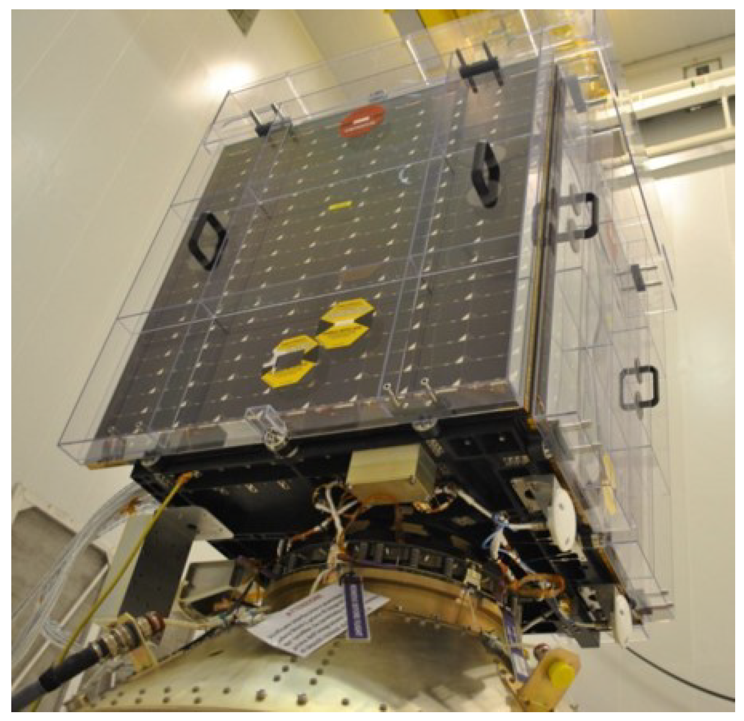
Abstract
:1. Introduction
2. Materials and Methods
2.1. Timepix Series
- Timepix was developed within the Medipix2 collaboration [32]. It segments the sensor into a square matrix of 256 × 256 pixels with a pixel pitch of 55 µm and purely relies on a frame-based readout scheme (dead-time > 11 ms). Each of the 65,536 pixels can be set to either of the three modes of signal processing: time-over-threshold (ToT), time-of-arrival (ToA, resolution > 10 ns), and hit counting.
- Timepix2, while still relying on the frame-based readout, provides additional features, e.g., a simultaneous measurement of ToA and ToT and an adaptive gain ToT mode for improved spectroscopy at high-energy deposition [33].
- The key improvements of Timepix3 are a time resolution below 2 ns and the data-driven mode. The latter provides an almost dead-time-free detector operation by reading out only the pixels, which are actually triggered by an ionizing particle, while all other pixels remain active (per-pixel dead time: ∼475 ns). Pixel hit rates up to 80 MHits s−1 can be sent off a chip at a bandwidth of 5.12 Gbps.
- Timepix4 comes with an increased pixel matrix featuring 512 × 448 pixels with a pitch of 55 µm (resulting in an area of ∼7 cm2) [31]. Similar to Timepix3, it offers frame-based and data-driven readout schemes, but with 8 × higher maximal hit rate. The time binning is improved to 195 ps. The readout bandwidth can be up to 164 Gbps.
2.2. The Space Application of Timepix Radiation Monitor (SATRAM)
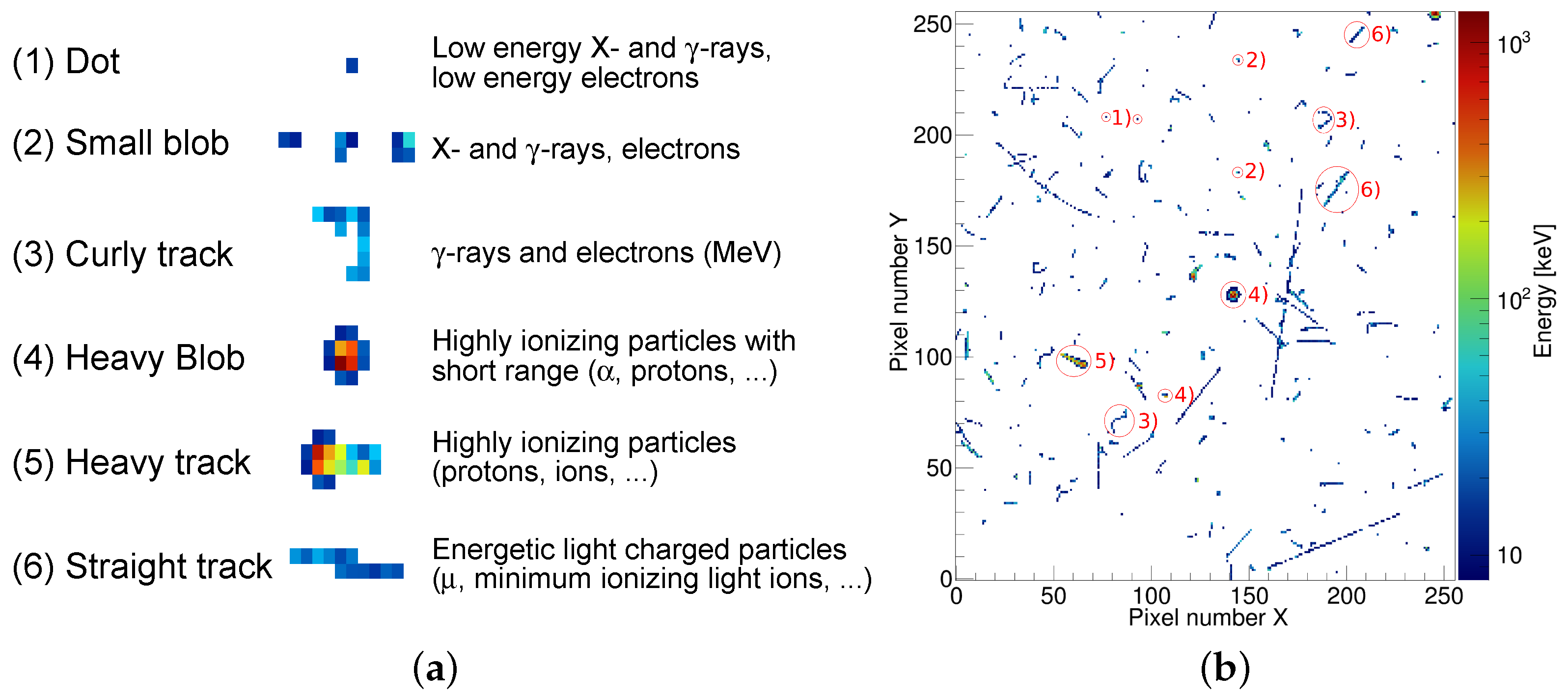
2.3. Pattern Recognition Tools and Particle Separation
- The number of pixels in the cluster N;
- The deposited energy is defined as the sum of energies measured in each pixel of a cluster ;
- The maximal energy measured in a single pixel of the cluster ;
- The linearity of the cluster, which is defined as the relative amount of pixel lying within a distance of one pixel from the longest line segment between two pixels of the cluster;
- The roundness of the cluster;
- The average number of neighboring pixels;
- The sum of the absolute values of cubic and quadratic terms of a third-order polynomial fit of the cluster.
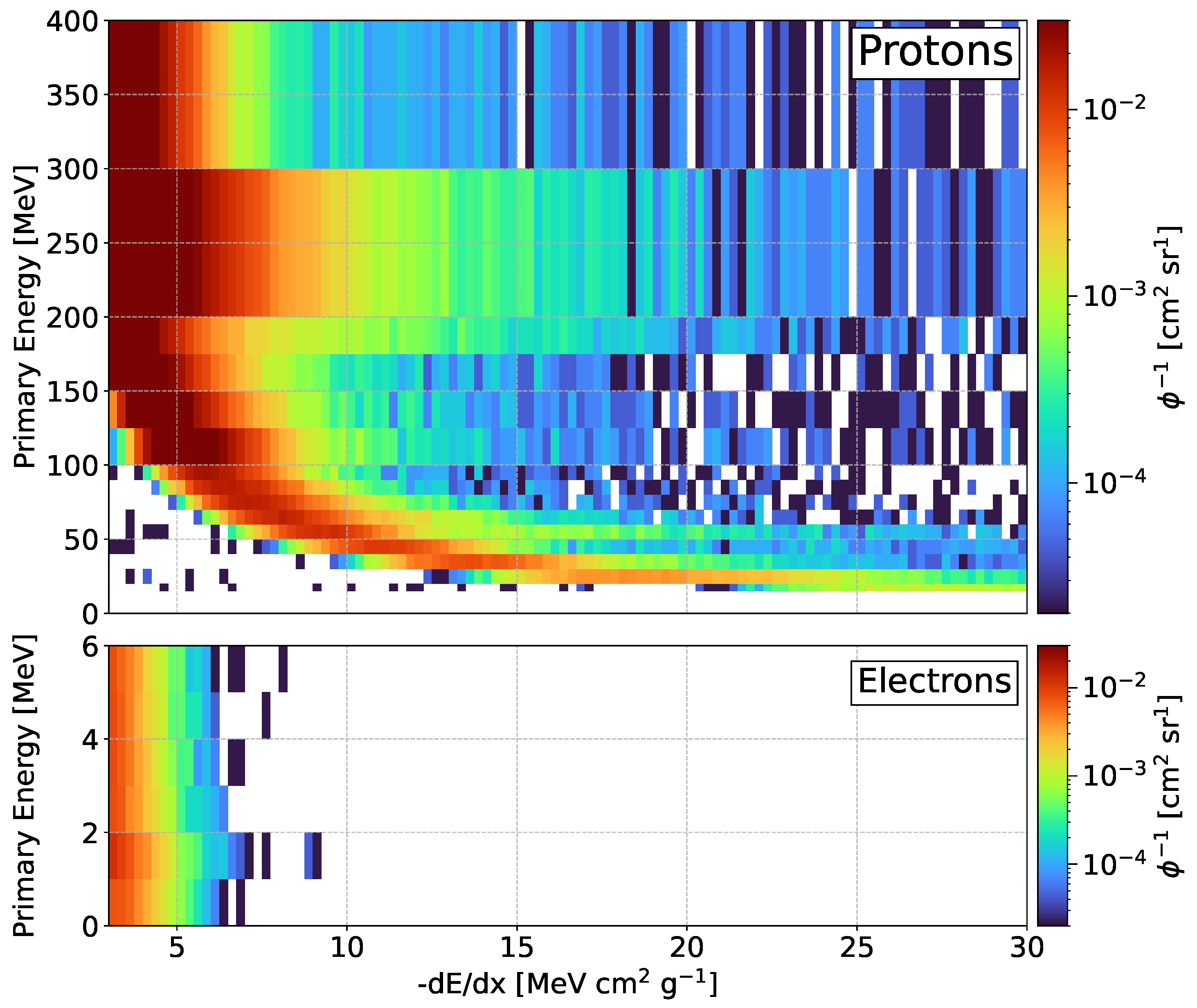
2.4. dE/dX Spectrum Unfolding
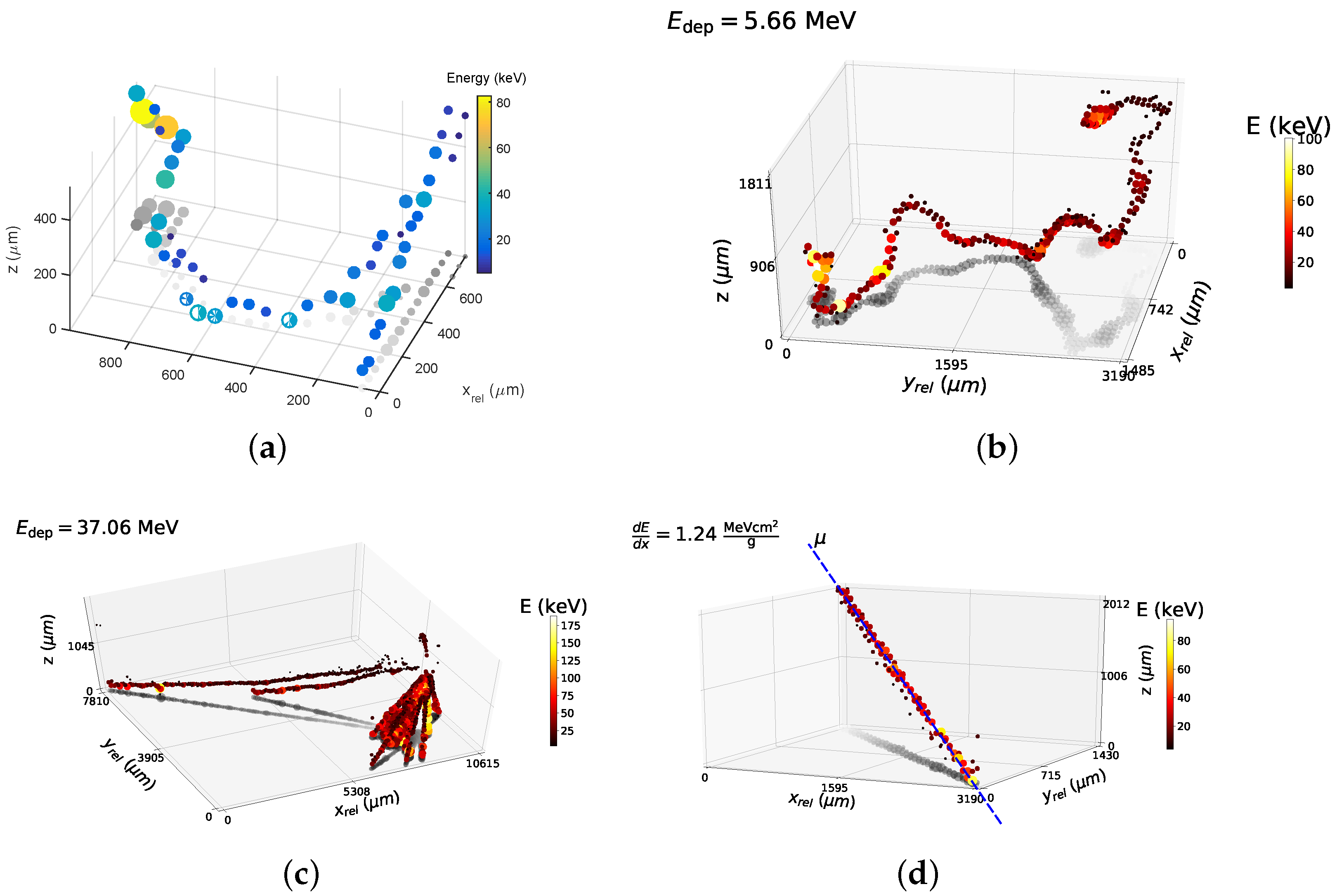
2.5. 3D Reconstruction of Particle Traces within the Semiconductor Sensor—Use as a Solid State Time Projection Chamber
2.6. Single-Layer Compton Camera and Scatter Polarimetry
3. Results
3.1. Space Heritage—SATRAM and Its 10 Years of Operation as a Radiation Monitor
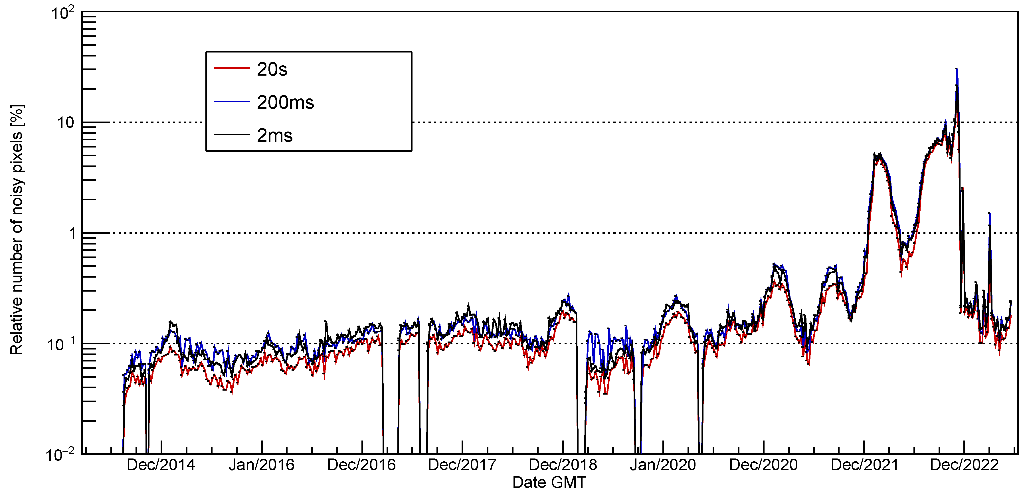
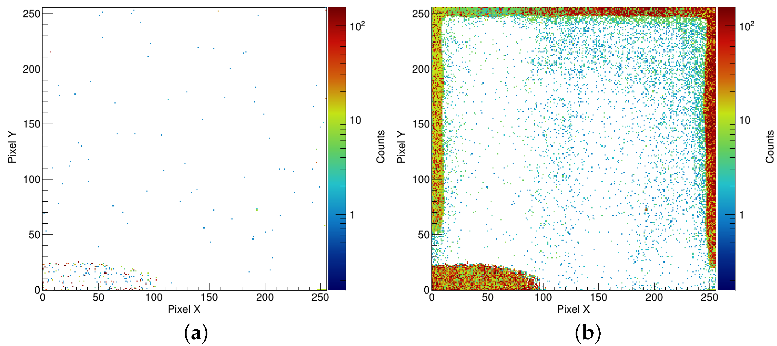
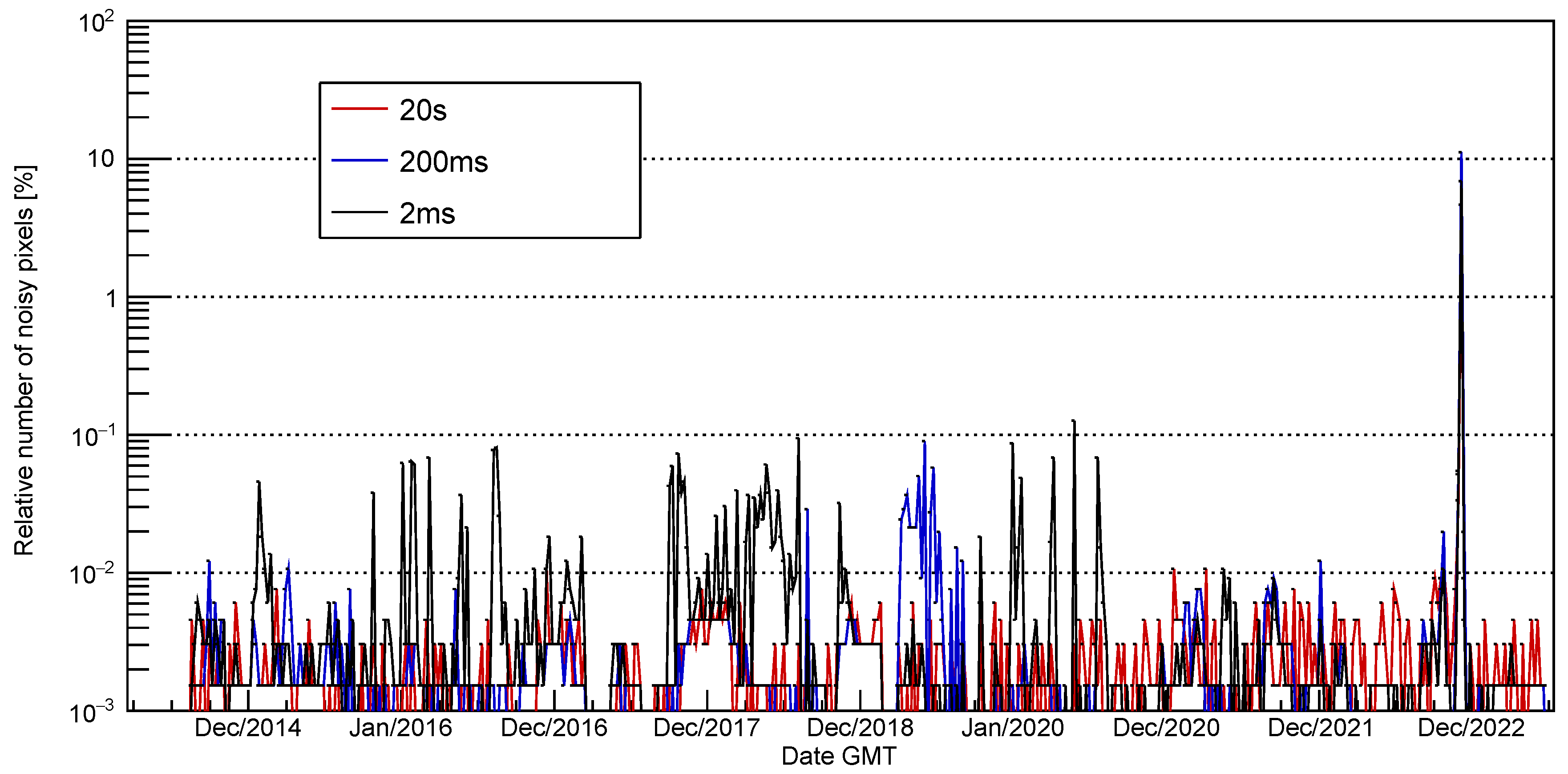
3.1.1. Measurement Stability—Noisy Pixel Appearance and Removal
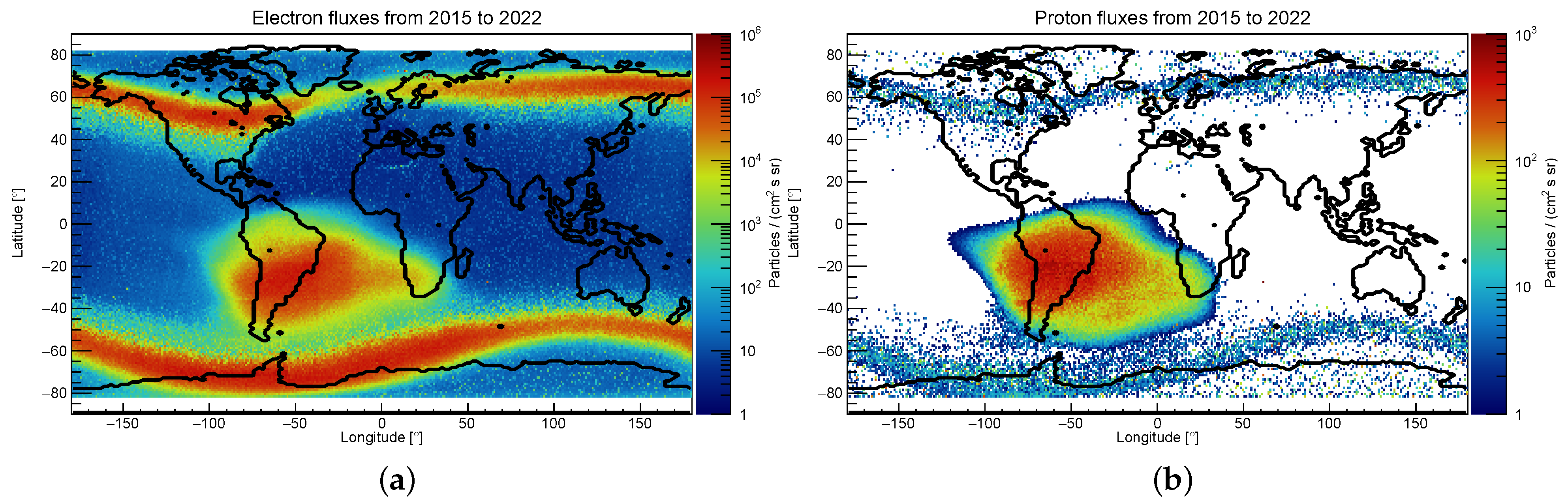
3.1.2. Mapping Out Electron and Proton Fluxes in Orbit
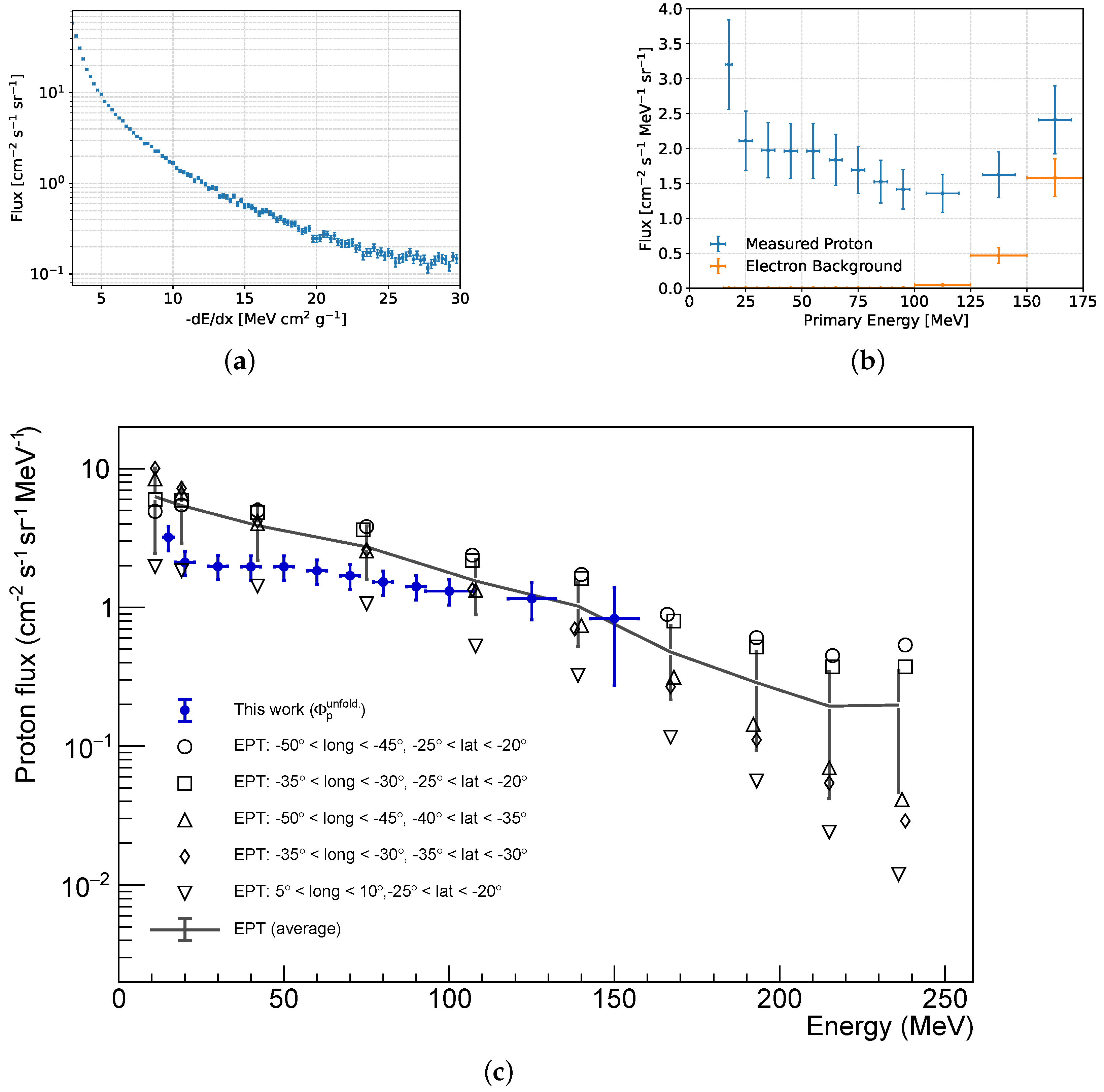
3.1.3. Measurement of the Proton Spectrum in the SAA
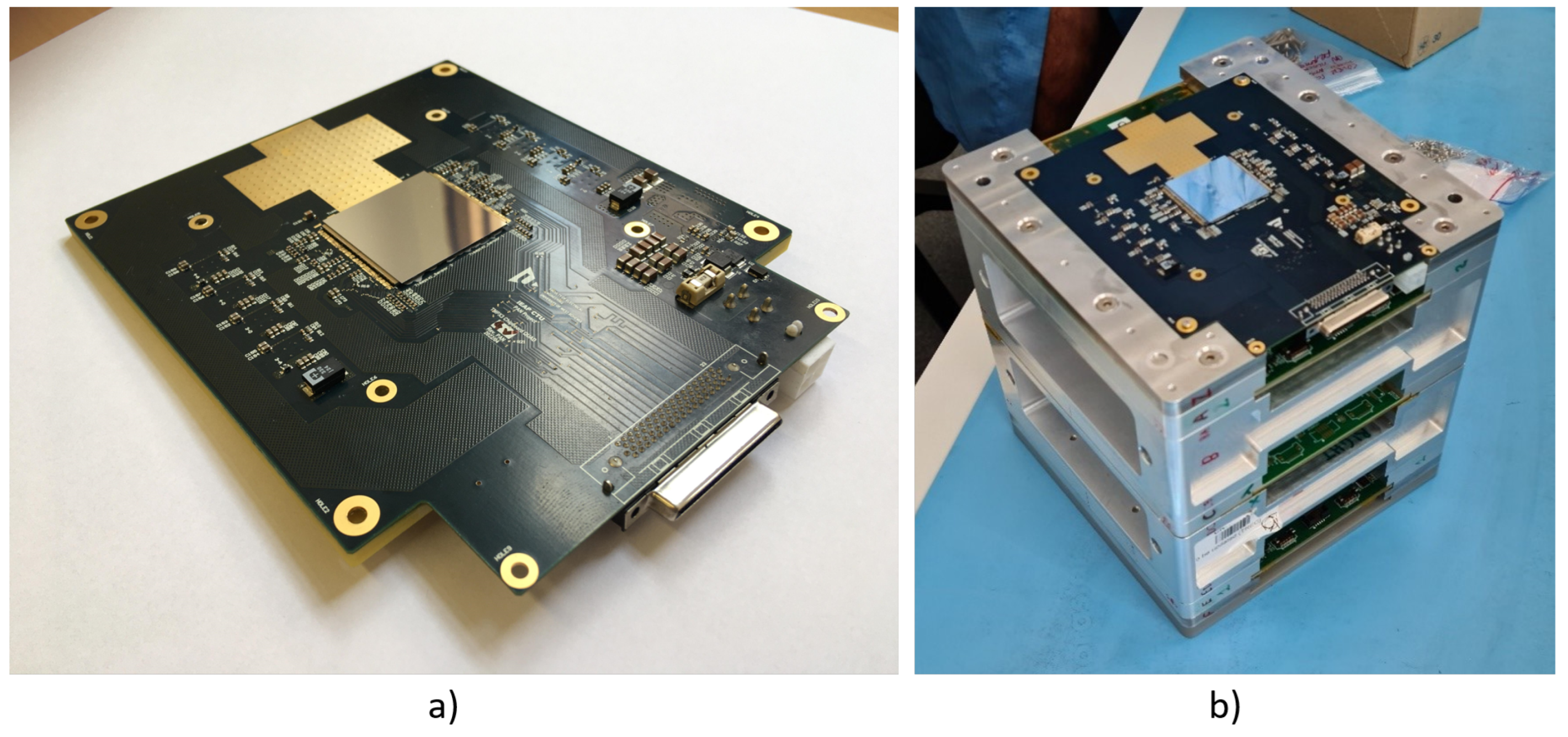
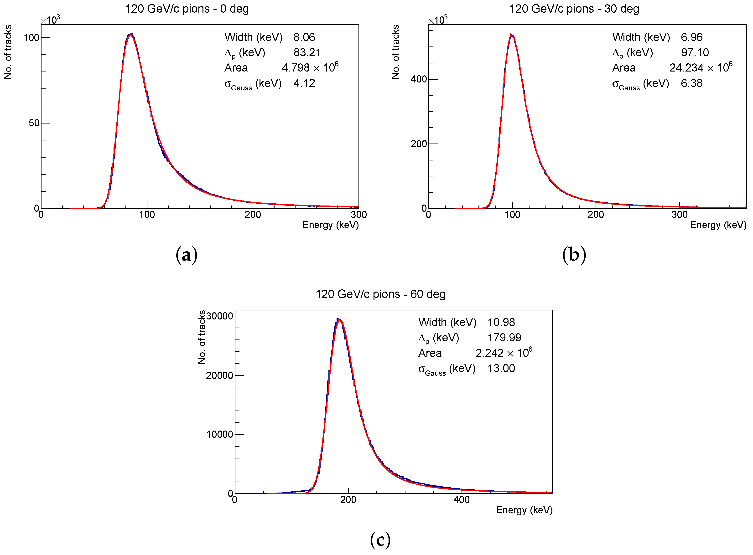
3.2. Large Area Timepix3 Detectors as Tracking Modules in a Magnetic Spectrometer
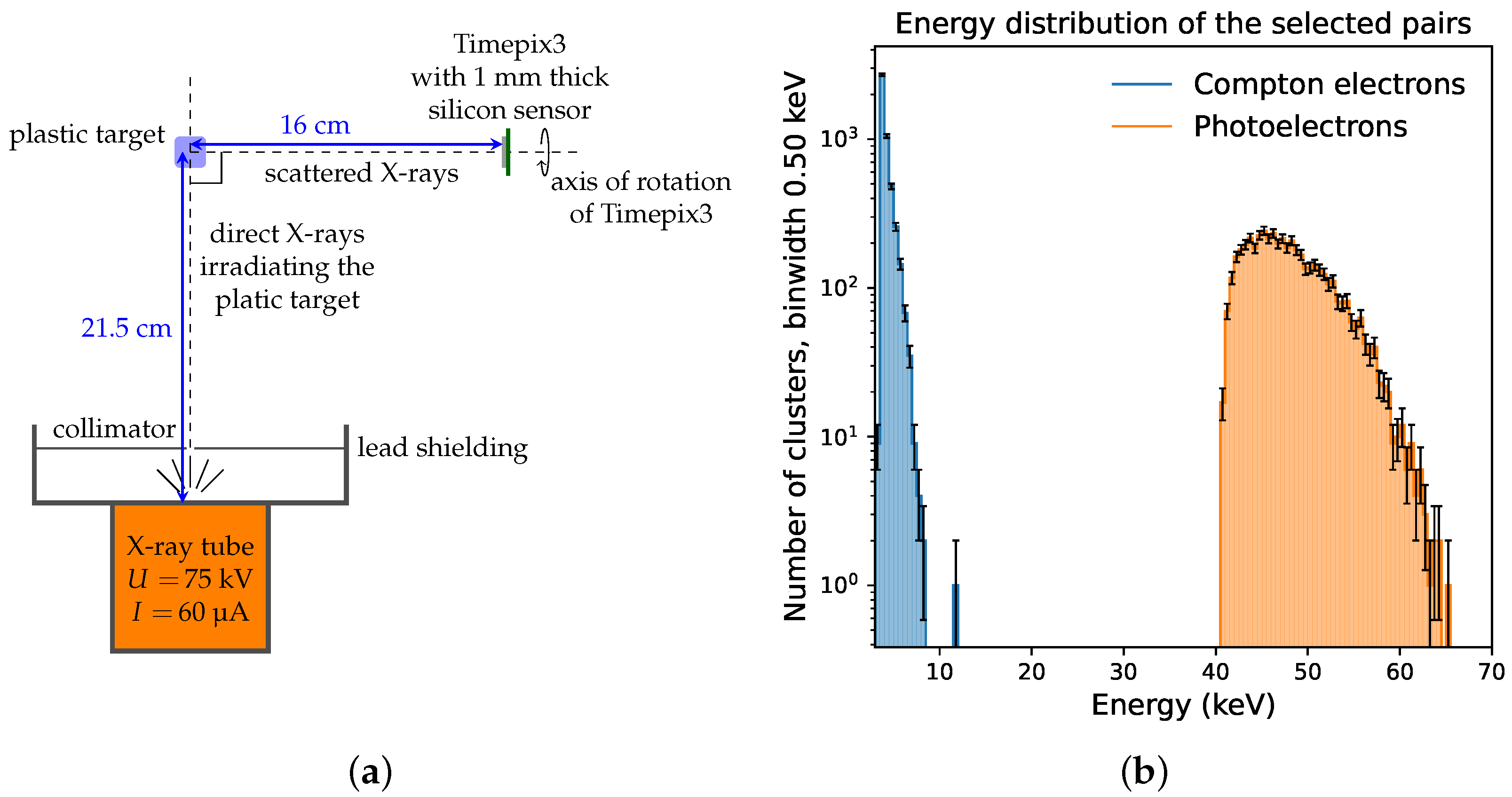
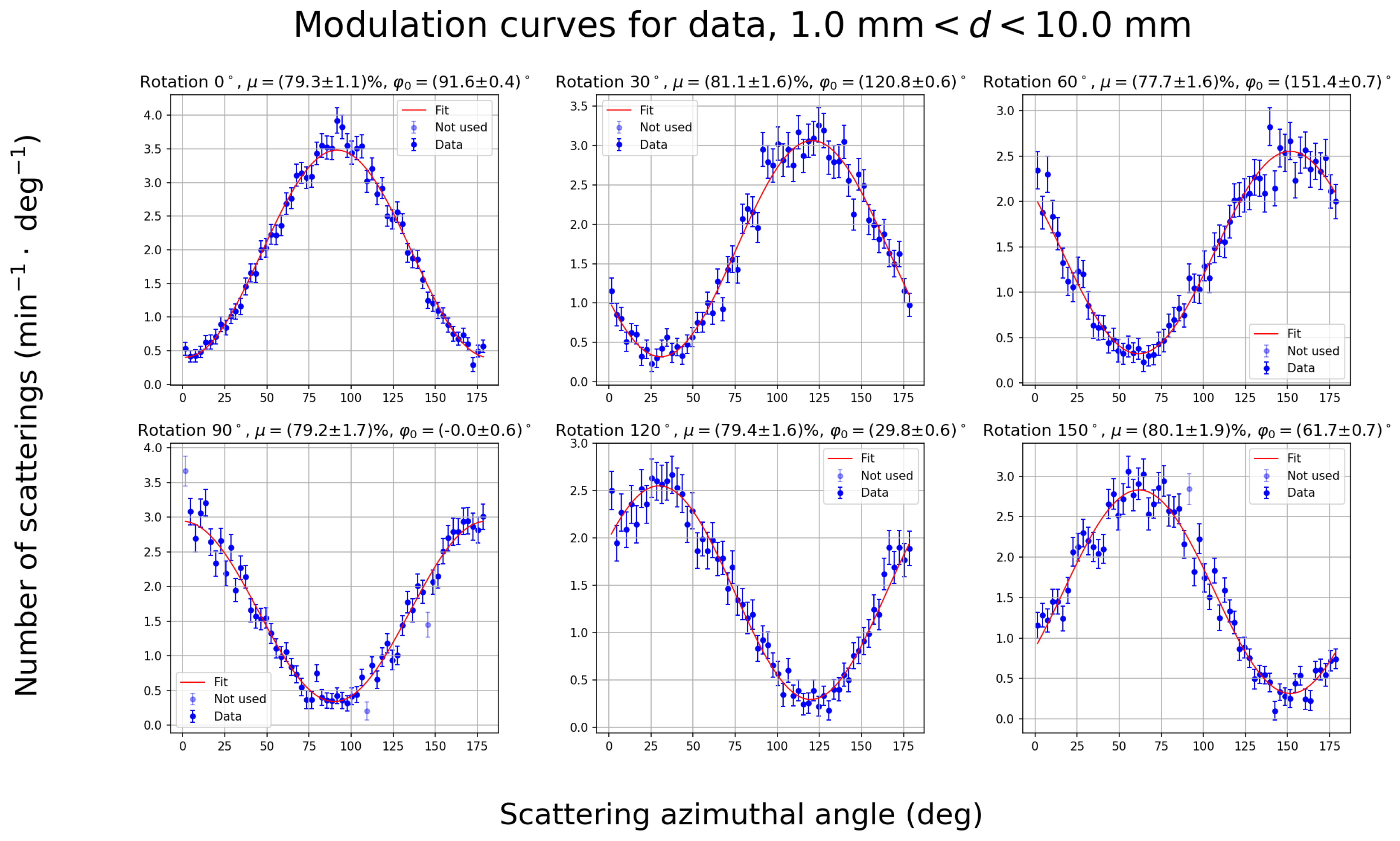
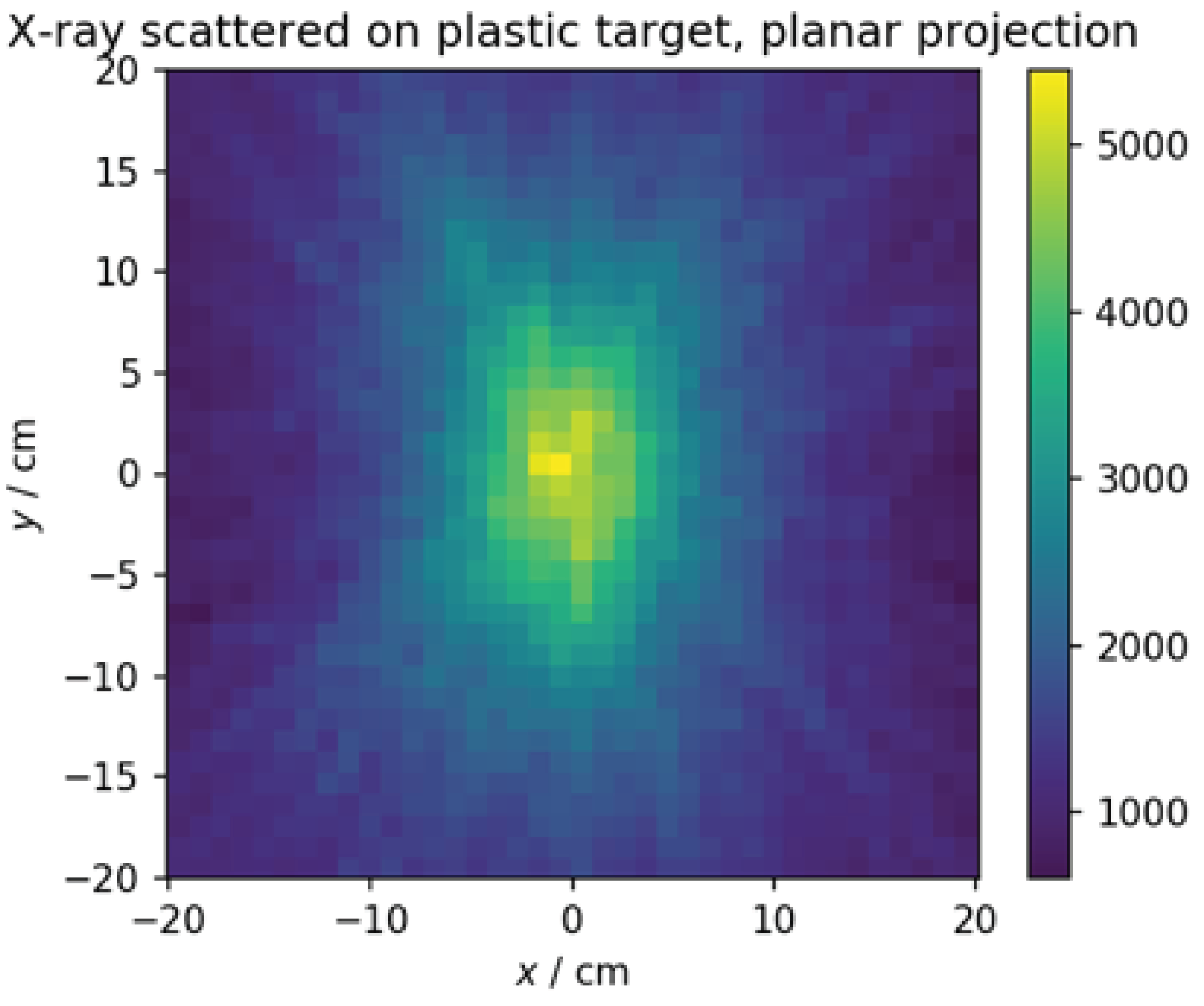
3.3. Capabilities of Timepix3 as a Compton Camera and Scatter Polarimeter
4. Discussion
4.1. Timepix-Based Radiation Monitors
4.2. Towards Astroparticle Physics Application
4.2.1. From Mini.PAN to Pix.PAN
4.2.2. Compton Scatter Polarimetry
5. Conclusions
Author Contributions
Funding
Data Availability Statement
Acknowledgments
Conflicts of Interest
Abbreviations
| ASIC | Application-Specific Integrated Circuit |
| CdTe | Cadmiumtelluride |
| CZT | Cadmiumzinctelluride |
| GaAs:Cr | Chromium-Compensated Galliumarsenide |
| CNN | Convolution Neural Network |
| ESA | European Space Agency |
| EPT | Energetic Particle Telescope |
| HITPix | Highly Integrated Timepix radiation monitor |
| HPD | Hybrid pixel detector |
| ICARE | Influence sur les Composants Avancés des Radiations de l’Espace |
| LEO | Low Earth Orbit |
| MIRAM | Miniaturized Radiation Monitor |
| MS | Magnetic Spectrometer |
| MPD | Minimum Detectable Polarization |
| NN | Neural Network |
| PAN | Penetrating Particle Analyzer |
| SAA | South Atlantic Anomaly |
| SATRAM | Space Application Timepix Radiation Monitor |
| SPENVIS | Space Environment Information System |
| SREM | Standard Radiation Environment Monitor |
| SWIMMR | Space Weather Instrumentation, Measurement, Modelling and Risk |
References
- Campbell, M. 10 years of the Medipix2 Collaboration. Nucl. Instruments Methods Phys. Res. Sect. A Accel. Spectrometers Detect. Assoc. Equip. 2011, 633, S1–S10. [Google Scholar] [CrossRef]
- Campbell, M.; Heijne, E.; Llopart, X.; Colas, P.; Giganon, A.; Giomataris, Y.; Chefdeville, M.; Colijn, A.; Fornaini, A.; van der Graaf, H.; et al. GOSSIP: A vertex detector combining a thin gas layer as signal generator with a CMOS readout pixel array. Nucl. Instruments Methods Phys. Res. Sect. A Accel. Spectrometers Detect. Assoc. Equip. 2006, 560, 131–134. [Google Scholar] [CrossRef]
- Bamberger, A.; Desch, K.; Renz, U.; Titov, M.; Vlasov, N.; Wienemann, P.; Zwerger, A. Resolution studies on 5GeV electron tracks observed with triple-GEM and MediPix2/TimePix-readout. Nucl. Instruments Methods Phys. Res. Sect. A Accel. Spectrometers Detect. Assoc. Equip. 2007, 581, 274–278. [Google Scholar] [CrossRef]
- George, S.; Murtas, F.; Alozy, J.; Curioni, A.; Rosenfeld, A.; Silari, M. Particle tracking with a Timepix based triple GEM detector. J. Instrum. 2015, 10, P11003. [Google Scholar] [CrossRef]
- Ballabriga, R.; Campbell, M.; Llopart, X. Asic developments for radiation imaging applications: The medipix and timepix family. Nucl. Instruments Methods Phys. Res. Sect. A Accel. Spectrometers Detect. Assoc. Equip. 2018, 878, 10–23. [Google Scholar] [CrossRef]
- Jakůbek, J. Semiconductor Pixel detectors and their applications in life sciences. J. Instrum. 2009, 4, P03013. [Google Scholar] [CrossRef]
- Llopart, X.; Ballabriga, R.; Campbell, M.; Tlustos, L.; Wong, W. Timepix, a 65k programmable pixel readout chip for arrival time, energy and/or photon counting measurements. Nucl. Instruments Methods Phys. Res. Sect. A Accel. Spectrometers Detect. Assoc. Equip. 2007, 581, 485–494. [Google Scholar] [CrossRef]
- Poikela, T.; Plosila, J.; Westerlund, T.; Campbell, M.; De Gaspari, M.; Llopart, X.; Gromov, V.; Kluit, R.; Van Beuzekom, M.; Zappon, F.; et al. Timepix3: A 65K channel hybrid pixel readout chip with simultaneous ToA/ToT and sparse readout. J. Instrum. 2014, 9, C05013. [Google Scholar] [CrossRef]
- Stoffle, N.; Pinsky, L.; Kroupa, M.; Hoang, S.; Idarraga, J.; Amberboy, C.; Rios, R.; Hauss, J.; Keller, J.; Bahadori, A.; et al. Timepix-based radiation environment monitor measurements aboard the International Space Station. Nucl. Instruments Methods Phys. Res. Sect. A Accel. Spectrometers Detect. Assoc. Equip. 2015, 782, 143–148. [Google Scholar] [CrossRef]
- Kroupa, M.; Bahadori, A.; Campbell-Ricketts, T.; Empl, A.; Hoang, S.M.; Idarraga-Munoz, J.; Rios, R.; Semones, E.; Stoffle, N.; Tlustos, L.; et al. A semiconductor radiation imaging pixel detector for space radiation dosimetry. Life Sci. Space Res. 2015, 6, 69–78. [Google Scholar] [CrossRef] [PubMed]
- Kroupa, M.; Campbell-Ricketts, T.; Bahadori, A.A.; Pal Chowdhury, R.; Empl, A.; George, S.P.; O’Brien, T.P. Extravehicular Electron Measurement Based on an Intravehicular Pixel Detector. J. Geophys. Res. Space Phys. 2019, 124, 8271–8279. [Google Scholar] [CrossRef]
- Granja, C.; Polansky, S.; Vykydal, Z.; Pospisil, S.; Owens, A.; Kozacek, Z.; Mellab, K.; Simcak, M. The SATRAM Timepix spacecraft payload in open space on board the Proba-V satellite for wide range radiation monitoring in LEO orbit. Planet. Space Sci. 2016, 125, 114–129. [Google Scholar] [CrossRef]
- Granja, C.; Polansky, S.; Vykydal, Z.; Pospisil, S.; Turecek, D.; Owens, A.; Mellab, K.; Nieminen, P.; Dvorak, Z.; Simcak, M.; et al. Quantum imaging monitoring and directional visualization of space radiation with timepix based SATRAM spacecraft payload in open space on board the ESA Proba-V satellite. In Proceedings of the 2014 IEEE Nuclear Science Symposium and Medical Imaging Conference (NSS/MIC), Seattle, WA, USA, 8–15 November 2014; pp. 1–2. [Google Scholar] [CrossRef]
- Gohl, S.; Bergmann, B.; Evans, H.; Nieminen, P.; Owens, A.; Posipsil, S. Study of the radiation fields in LEO with the Space Application of Timepix Radiation Monitor (SATRAM). Adv. Space Res. 2019, 63, 1646–1660. [Google Scholar] [CrossRef]
- Gohl, S.; Bergmann, B.; Kaplan, M.; Němec, F. Measurement of electron fluxes in a Low Earth Orbit with SATRAM and comparison to EPT data. Adv. Space Res. 2023, 72, 2362–2376. [Google Scholar] [CrossRef]
- Ruffenach, M.; Bourdarie, S.; Bergmann, B.; Gohl, S.; Mekki, J.; Vaillé, J. A New Technique Based on Convolutional Neural Networks to Measure the Energy of Protons and Electrons With a Single Timepix Detector. IEEE Trans. Nucl. Sci. 2021, 68, 1746–1753. [Google Scholar] [CrossRef]
- Furnell, W.; Shenoy, A.; Fox, E.; Hatfield, P. First results from the LUCID-Timepix spacecraft payload onboard the TechDemoSat-1 satellite in Low Earth Orbit. Adv. Space Res. 2019, 63, 1523–1540. [Google Scholar] [CrossRef]
- Gohl, S.; Bergmann, B.; Pospisil, S. Design Study of a New Miniaturized Radiation Monitor Based on Previous Experience with the Space Application of the Timepix Radiation Monitor (SATRAM). In Proceedings of the 2018 IEEE Nuclear Science Symposium and Medical Imaging Conference Proceedings (NSS/MIC), Sydney, NSW, Australia, 10–17 November 2018; pp. 1–7. [Google Scholar] [CrossRef]
- Wong, W.; Alozy, J.; Ballabriga, R.; Campbell, M.; Kremastiotis, I.; Llopart, X.; Poikela, T.; Sriskaran, V.; Tlustos, L.; Turecek, D. Introducing Timepix2, a frame-based pixel detector readout ASIC measuring energy deposition and arrival time. Radiat. Meas. 2020, 131, 106230. [Google Scholar] [CrossRef]
- RAL Space SWIMMR-1. Available online: https://www.ralspace.stfc.ac.uk/Pages/SWIMMR-1-launches-in-boost-to-UK-space-weather-forecasting-capabilities.aspx (accessed on 26 October 2023).
- Filgas, R.; (Institute of Experimental and Applied Physics, Czech Technical University, Prague, Czechia). Private communication, 2023.
- Wu, X.; Ambrosi, G.; Azzarello, P.; Bergmann, B.; Bertucci, B.; Cadoux, F.; Campbell, M.; Duranti, M.; Ionica, M.; Kole, M.; et al. Penetrating particle ANalyzer (PAN). Adv. Space Res. 2019, 63, 2672–2682. [Google Scholar] [CrossRef]
- Bergmann, B.; Pichotka, M.; Pospisil, S.; Vycpalek, J.; Burian, P.; Broulim, P.; Jakubek, J. 3D track reconstruction capability of a silicon hybrid active pixel detector. Eur. Phys. J. C 2017, 77, 421. [Google Scholar] [CrossRef]
- Bergmann, B.; Burian, P.; Manek, P.; Pospisil, S. 3D reconstruction of particle tracks in a 2 mm thick CdTe hybrid pixel detector. Eur. Phys. J. C 2019, 79, 165. [Google Scholar] [CrossRef]
- Turecek, D.; Jakubek, J.; Trojanova, E.; Sefc, L. Single layer Compton camera based on Timepix3 technology. J. Instrum. 2020, 15, C01014. [Google Scholar] [CrossRef]
- Amoyal, G.; Schoepff, V.; Carrel, F.; Michel, M.; Blanc de Lanaute, N.; Angélique, J. Development of a hybrid gamma camera based on Timepix3 for nuclear industry applications. Nucl. Instruments Methods Phys. Res. Sect. A Accel. Spectrometers Detect. Assoc. Equip. 2021, 987, 164838. [Google Scholar] [CrossRef]
- Wen, J.; Zheng, X.; Gao, H.; Zeng, M.; Zhang, Y.; Yu, M.; Wu, Y.; Cang, J.; Ma, G.; Zhao, Z. Optimization of Timepix3-based conventional Compton camera using electron track algorithm. Nucl. Instruments Methods Phys. Res. Sect. A Accel. Spectrometers Detect. Assoc. Equip. 2022, 1021, 165954. [Google Scholar] [CrossRef]
- Carenza, P.; la Torre Luque, P.D. Detecting neutrino-boosted axion dark matter in the MeV gap. Eur. Phys. J. C 2023, 83. [Google Scholar] [CrossRef]
- Caroli, E.; Moita, M.; Da Silva, R.M.C.; Del Sordo, S.; De Cesare, G.; Maia, J.M.; Pàscoa, M. Hard X-ray and Soft Gamma Ray Polarimetry with CdTe/CZT Spectro-Imager. Galaxies 2018, 6, 69. [Google Scholar] [CrossRef]
- Weisskopf, M.C. An Overview of X-Ray Polarimetry of Astronomical Sources. Galaxies 2018, 6, 33. [Google Scholar] [CrossRef]
- Llopart, X.; Alozy, J.; Ballabriga, R.; Campbell, M.; Casanova, R.; Gromov, V.; Heijne, E.; Poikela, T.; Santin, E.; Sriskaran, V.; et al. Timepix4, a large area pixel detector readout chip which can be tiled on 4 sides providing sub-200 ps timestamp binning. J. Instrum. 2022, 17, C01044. [Google Scholar] [CrossRef]
- Medipix Collaboration. Available online: https://medipix.web.cern.ch/home (accessed on 18 July 2023).
- Bergmann, B.; Smolyanskiy, P.; Burian, P.; Pospisil, S. Experimental study of the adaptive gain feature for improved position-sensitive ion spectroscopy with Timepix2. J. Instrum. 2022, 17, C01025. [Google Scholar] [CrossRef]
- Boscher, D.; Bourdarie, S.A.; Falguere, D.; Lazaro, D.; Bourdoux, P.; Baldran, T.; Rolland, G.; Lorfevre, E.; Ecoffet, R. In Flight Measurements of Radiation Environment on Board the French Satellite JASON-2. IEEE Trans. Nucl. Sci. 2011, 58, 916–922. [Google Scholar] [CrossRef]
- Boscher, D.; Cayton, T.; Maget, V.; Bourdarie, S.; Lazaro, D.; Baldran, T.; Bourdoux, P.; Lorfèvre, E.; Rolland, G.; Ecoffet, R. In-Flight Measurements of Radiation Environment on Board the Argentinean Satellite SAC-D. IEEE Trans. Nucl. Sci. 2014, 61, 3395–3400. [Google Scholar] [CrossRef]
- Evans, H.; Bühler, P.; Hajdas, W.; Daly, E.; Nieminen, P.; Mohammadzadeh, A. Results from the ESA SREM monitors and comparison with existing radiation belt models. Adv. Space Res. 2008, 42, 1527–1537. [Google Scholar] [CrossRef]
- Sandberg, I.; Daglis, I.A.; Anastasiadis, A.; Bühler, P.; Nieminen, P.; Evans, H. Unfolding and validation of SREM fluxes. In Proceedings of the 2011 12th European Conference on Radiation and Its Effects on Components and Systems, Seville, Spain, 19–23 September 2011; pp. 599–606. [Google Scholar] [CrossRef]
- Holy, T.; Heijne, E.; Jakubek, J.; Pospisil, S.; Uher, J.; Vykydal, Z. Pattern recognition of tracks induced by individual quanta of ionizing radiation in Medipix2 silicon detector. Nucl. Instruments Methods Phys. Res. Sect. A Accel. Spectrometers Detect. Assoc. Equip. 2008, 591, 287–290. [Google Scholar] [CrossRef]
- Tensorflow. Available online: https://www.tensorflow.org/ (accessed on 9 September 2023).
- D’Agostini, G. Improved iterative Bayesian unfolding. arXiv 2010, arXiv:1010.0632. [Google Scholar]
- Brenner, L.; Verschuuren, P.; Balasubramanian, R.; Burgard, C.; Croft, V.; Cowan, G.; Verkerke, W. RooUnfold: ROOT Unfolding Framework. 2020. Available online: https://gitlab.cern.ch/RooUnfold/RooUnfold (accessed on 9 September 2023).
- Kroupa, M.; Bahadori, A.A.; Campbell-Ricketts, T.; George, S.P.; Zeitlin, C. Kinetic energy reconstruction with a single layer particle telescope. Appl. Phys. Lett. 2018, 112, 134103. [Google Scholar] [CrossRef]
- Kroupa, M.; Bahadori, A.A.; Campbell-Ricketts, T.; George, S.P.; Stoffle, N.; Zeitlin, C. Light ion isotope identification in space using a pixel detector based single layer telescope. Appl. Phys. Lett. 2018, 113, 174101. [Google Scholar] [CrossRef]
- Agostinelli, S.; Allison, J.; Amako, K.; Apostolakis, J.; Araujo, H.; Arce, P.; Asai, M.; Axen, D.; Banerjee, S.; Barrand, G.; et al. Geant4—A simulation toolkit. Nucl. Instruments Methods Phys. Res. Sect. A Accel. Spectrometers Detect. Assoc. Equip. 2003, 506, 250–303. [Google Scholar] [CrossRef]
- Garvey, D. Advanced Methodology for Radiation Field Decomposition with Hybrid Pixel Detectors. Master’s Thesis, Faculty of Nuclear Sciences and Physical Engineering, Czech Technical University in Prague, Prague, Czechia, 2023. Available online: https://dspace.cvut.cz/handle/10467/108693 (accessed on 22 February 2024).
- Michel, T.; Durst, J.; Jakubek, J. X-ray polarimetry by means of Compton scattering in the sensor of a hybrid photon counting pixel detector. Nucl. Instruments Methods Phys. Res. Sect. A Accel. Spectrometers Detect. Assoc. Equip. 2009, 603, 384–392. [Google Scholar] [CrossRef]
- López Rosson, G.; Pierrard, V. Analysis of proton and electron spectra observed by EPT/PROBA-V in the South Atlantic Anomaly. Adv. Space Res. 2017, 60, 796–805. [Google Scholar] [CrossRef]
- Farkas, M.; Bergmann, B.; Broulim, P.; Burian, P.; Ambrosi, G.; Azzarello, P.; Pušman, L.; Sitarz, M.; Smolyanskiy, P.; Sukhonos, D.; et al. Characterization of a Large Area Hybrid Pixel Detector of Timepix3 Technology for Space Applications. Instruments 2024, 8, 11. [Google Scholar] [CrossRef]
- Jordan, C.E. RADEX INC BEDFORD MA, Contract No F19628-89-C-0068. Available online: https://apps.dtic.mil/sti/citations/tr/ADA223660 (accessed on 26 October 2023).
- Ginet, G.P.; O’Brien, T.P.; Huston, S.L.; Johnston, W.R.; Guild, T.B.; Friedel, R.; Lindstrom, C.D.; Roth, C.J.; Whelan, P.; Quinn, R.A.; et al. AE9, AP9 and SPM: New Models for Specifying the Trapped Energetic Particle and Space Plasma Environment. In The Van Allen Probes Mission; Fox, N., Burch, J.L., Eds.; Springer: Boston, MA, USA, 2014; pp. 579–615. [Google Scholar] [CrossRef]
- Hulsmann, J.; Wu, X.; Azzarello, P.; Bergmann, B.; Campbell, M.; Clark, G.; Cadoux, F.; Ilzawa, T.; Kollmann, P.; Llopart, X. Relativistic Particle Measurements in Jupiter’s Magnetosphere with Pix.PAN. Exp. Astron. 2023, 56, 371–402. [Google Scholar] [CrossRef]
- Smolyanskiy, P.; Bergmann, B.; Burian, P.; Cherlin, A.; Jelínek, J.; Maneuski, D.; Pospíšil, S.; O’Shea, V. Characterization of a 5 mm thick CZT-Timepix3 pixel detector for energy-dispersive γ-ray and particle tracking. Phys. Scr. 2023, 99, 015301. [Google Scholar] [CrossRef]
- Useche, S.J.; Roque, G.A.; Schütz, M.K.; Fiederle, M.; Procz, S. Characterization of a 5mm thick CdTe photon-counting detector: Advancing nuclear decommissioning with Compton camera technology. In Proceedings of the 2023 IEEE Nuclear Science Symposium, Medical Imaging Conference and International Symposium on Room-Temperature Semiconductor Detectors (NSS MIC RTSD), Vancouver, BC, Canada, 4–11 November 2023; p. 1. [Google Scholar] [CrossRef]


Disclaimer/Publisher’s Note: The statements, opinions and data contained in all publications are solely those of the individual author(s) and contributor(s) and not of MDPI and/or the editor(s). MDPI and/or the editor(s) disclaim responsibility for any injury to people or property resulting from any ideas, methods, instructions or products referred to in the content. |
© 2024 by the authors. Licensee MDPI, Basel, Switzerland. This article is an open access article distributed under the terms and conditions of the Creative Commons Attribution (CC BY) license (https://creativecommons.org/licenses/by/4.0/).
Share and Cite
Bergmann, B.; Gohl, S.; Garvey, D.; Jelínek, J.; Smolyanskiy, P. Results and Perspectives of Timepix Detectors in Space—From Radiation Monitoring in Low Earth Orbit to Astroparticle Physics. Instruments 2024, 8, 17. https://doi.org/10.3390/instruments8010017
Bergmann B, Gohl S, Garvey D, Jelínek J, Smolyanskiy P. Results and Perspectives of Timepix Detectors in Space—From Radiation Monitoring in Low Earth Orbit to Astroparticle Physics. Instruments. 2024; 8(1):17. https://doi.org/10.3390/instruments8010017
Chicago/Turabian StyleBergmann, Benedikt, Stefan Gohl, Declan Garvey, Jindřich Jelínek, and Petr Smolyanskiy. 2024. "Results and Perspectives of Timepix Detectors in Space—From Radiation Monitoring in Low Earth Orbit to Astroparticle Physics" Instruments 8, no. 1: 17. https://doi.org/10.3390/instruments8010017