

Scattering Polarimetry in the Hard X-ray Range


Istituto di Astrofisica e Planetologia Spaziali-INAF, Via del Fosso del Cavaliere 100, 00133 Roma, Italy
Instruments 2024, 8(1), 20; https://doi.org/10.3390/instruments8010020
Submission received: 7 January 2024
/
Revised: 11 February 2024
/
Accepted: 13 February 2024
/
Published: 2 March 2024
(This article belongs to the Special Issue Advances in Space AstroParticle Physics: Frontier Technologies for Particle Measurements in Space)
Abstract
:In one and a half years, the Imaging X-ray Polarimetry Explorer has demonstrated the role and the potentiality of Polarimetry in X-ray Astronomy. The next steps include extension to higher energies. There is margin for an extension of the photoelectric approach up to 20–25 keV, but above that energy the only technique is Compton Scattering. Grazing incidence optics can focus photons up to 80 keV, not excluding a marginal extension to 150–200 keV. Given the physical constraints involved, the passage from photoelectric to scattering approach can make less effective the use of optics because of the high background. I discuss the choices in terms of detector design to mitigate the problem and the guidelines for future technological developments.
1. Introduction
Results of the Imaging Polarimetry Explorer eventually demonstrated, after 60 years of predictions, that X-ray polarimetry can be a powerful diagnostic for most classes of sources in the domain of High Energy Astrophysics. A short history of this subject can be found in [1]. The breakthrough performance of IXPE is due to a detector exploiting the photoelectric process. Measuring both the interaction point and the angle, the Gas Pixel Detector is suitable to be used as a focal plane detector [2]. For the future, we can predict a more extensive use of polarimetry techniques in X-ray Astronomy. This can include:
- a better exploitation in the IXPE band, with a larger area, as in the enhanced X-ray Timing and Polarimetry Mission [3], better angular resolution and faster operations, and
- the design of wide field instruments.
But both theoretic predictions and IXPE data suggest that an important step forward is the opening of the band above 10 keV. The photoelectric technique can be extended up to 20–25 keV [4,5], but most of instruments are based on scattering. Extensive reviews of scattering polarimetry can be found in Chattopadhyay (2021), Del Monte (2023) [6,7] and, for Gamma-Ray Bursts, in McConnell (2017) [8]. In this paper, I discuss how and when a polarimeter based on Compton scattering was and can be conceived, which implementations have been realized so far and which technical developments are needed in view of another future breakthrough. Conceptually every Compton Telescope, namely every instrument conceived to derive the direction of a photon from the kinematics of Compton scattering between two detecting units of the instrument, is by definition also a polarimeter and is out of this presentation. I only discuss those instruments that can be considered as an extension of the IXPE band, so I neglect the instruments operating only above 100–150 keV.
2. Plenty of Configurations
Any polarimeter is based on an analyzer, namely a material subject to a physical process that depends on polarization, and all the needed equipment to define the direction of the input radiation to detect the output radiation and to record, somehow, the angle selected by the interaction. In the optical domain, this is typically a rotating filter interposed in the path from the optics to the detector. The modulation of the rate with angle, typically following a () law, is the basis of the measurement of polarization. This is named a dispersive polarimeter in the sense that each angle is sampled at one time and the measurement needs one (or possibly several) complete rotation to provide a result. Also, in the optical band, there may be filters or polarizing prisms at fixed angles. In this case, the polarimeter is sampling three or four angles of the modulation curve, and this is sufficient to measure the polarization at every moment. This is a not dispersive polarimeter. In general, a polarimeter based on scattering is composed of the following components:
- A scatterer, namely a block of material toward which the input radiation is conveyed by an optics or a collimator.
- An absorber, namely a detector capable to detect the scattered photon and possibly measure angles and energy. Depending on the experiment concept, the scatterer/absorber configuration can be single or multiple, namely replicated to achieve a large area.
A scattering polarimeter is not dispersive in the sense that most of the angles are sampled simultaneously. A major difference with respect to photoelectric polarimeters is that some angles are forbidden or covered non-uniformly for several reasons, including mechanical mounting, or the different self-absorption within the scatterer, and the geometry of detecting arrays. Consequently, the coverage of angles is different. This is the source of serious complications that can be faced in different ways but, in any case, make significantly cumbersome the analysis of data. On the basis of the physics of the interactions, we can also identify two groups:
- One phase: Same material for the analyzer (scatterer) and the absorber.
- Two phases: Different materials for the analyzer and the absorber.
Another way of subdividing is as follows:
- Active scatterer, when the scatterer is a detector to be put in coincidence with the absorber.
- Passive Scatterer, when the scatterer is an inert material.
A further division is the following:
- Wide field to monitor wide regions of the sky and detect sources from unpredicted directions, such as Gamma-Ray Burst.
- Narrow field to study a source at a time. These can include large area detectors with a collimator or instruments for the focal plane of a telescope.
Two last divisions are not strictly technical. A polarimeter can be one of the two:
- Dedicated: designed and built to perform polarimetry.
- Byproduct: designed and built for some other purpose also performing some polarimetry.
An instrument not designed for polarimetry can also offer some information on scattering events, so, in principle, can perform some polarimetry. Historically, some use of this type was proposed. These instruments as polarimeters are much less sensitive and/or reliable than a dedicated polarimeter but, of course, have more chances to arrive in the orbit. I name them byproduct. Lastly, a polarimeter can be the following:
- Stand-alone, namely aboard a dedicated satellite.
- Part of a multi-instrument payload.
The problem of systematics and of uneven coverage of angles is usually solved with the rotation of the instrument around the observation axis. Of course, this is not feasible with instruments devoted to Gamma-Ray Bursts, given that the direction is unknown. Also, byproduct polarimetry based on imagers cannot benefit from rotation. All these configurations have been proposed or studied. A few have been implemented. Very few have arrived to be real experiment. I mainly review these configurations and propose my personal view for the future.
3. Basic Statistics and Physics
3.1. The Basic Statistics
To discuss the various configurations, I recall the basic statistics of detection of polarization in a regime of Poisson distribution, that can be found in several publications as in Weisskopf (2010), Strohmayer (2013) or Muleri (2022) [9,10,11]. The parameter driving the observing strategy and quantifying the scientific performance is the Minimum Detectable Polarization, namely the polarization to be exceeded to keep the probability of statistical fluctuation below a certain value. The general convention is to offer the MDP at 99%,
where is the efficiency of the instrument, S the flux of the source, B is the background rate, T is observing time. is the modulation factor, the parameter measuring the response of the instrument to a 100% polarized source. = 1 for an ideal analyzer. Except the time, all the parameters in the equation are energy dependent and the proper convolution integrals should be used instead of the variable, but for the purpose of this discussion, I use this simplified formalism. Also, in the literature, as in the papers presenting the IXPE results, data are analyzed and results are shown with the formalism of Stokes Parameters, coherently with the use in other wavelengths. This has many advantages in performing the analysis and showing the results [11], but would be a useless complication here. So I will carry on the discussion in terms of Polarization Degree and Angle. Starting from the interaction cross-sections, I discuss the value that can be achieved for these parameters with the various above-mentioned configurations of scattering polarimeters.
3.2. The Basic Physics
I follow the approach of Fabiani (2014) [12]. From the Compton formula, the energy of the incoming photon E and the energy of the scattered photon E′ are connected through the polar scattering angle .
The difference E-E′ of the energy of the photons is given to an electron of the scatterer, which is stopped with a range much shorter than the interaction length of the X-ray photon. In practice, for the sake of discussion, with a reasonable approximation, we can assume a local energy loss for the electron the angular distributions for scattering on free electrons for the emerging photon.
The polarization of the incoming photon determines the azimuth distribution. The Klein Nishina formula,
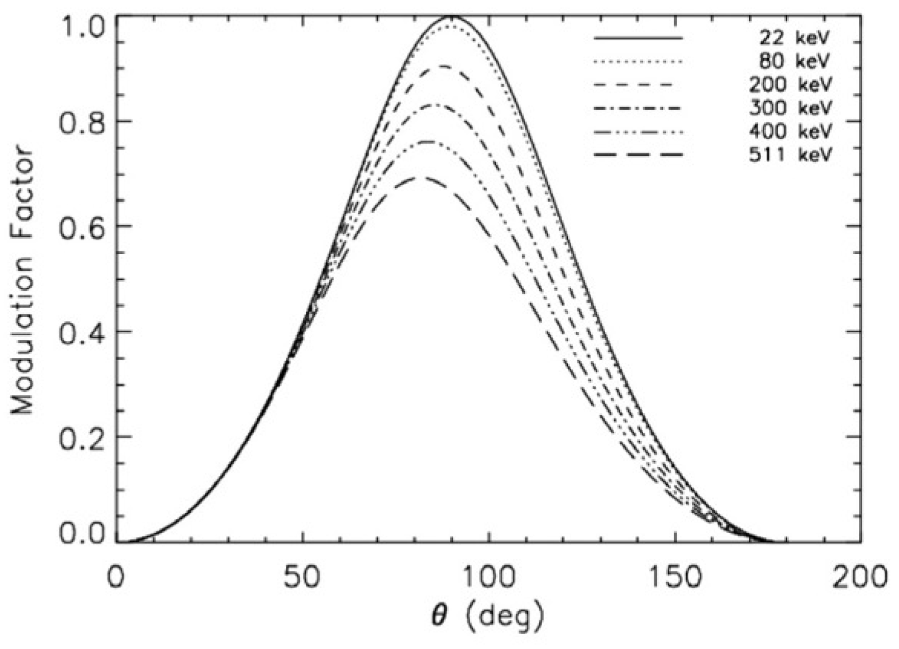
gives the angular distribution of the scattered photons. is the azimuth scattering angle. The distribution in is independent from polarization, while the distribution in is dependent and has the maximum for azimuth angle defining a plane of scattering perpendicular to the polarization of the photon. A complete treatment can be found in [13]. From these equations, the two distributions can be derived which are the most relevant for our discussion. One is the modulation (around azimuth angle ) as a function of the polar scattering angle and of the energy as shown in Figure 1.
From the figure, it is clear that, since is the parameter with the maximum impact on sensitivity in Equation (1), the photons scattered around 90° are the most useful ones. On the other side, the photons which are not collected do not contribute to efficiency . Every scattering polarimeter limits the accepted paths for the scattered photons, trying to optimize the MDP. The geometric configuration determines the scattering angles accepted and fixes the trade-off between the two parameters. Given that both and depend on energy, the trade-off configuration is energy dependent and the design of the experiment is based on a hypothetical optimization of the total scientific throughput of the mission. With a more ambitious approach, viable with nowadays technology, when the point of scattering and the point of absorption can be measured, this information can be used by assigning to each event a weight (substantially proportional to ), but this is not easy at all.
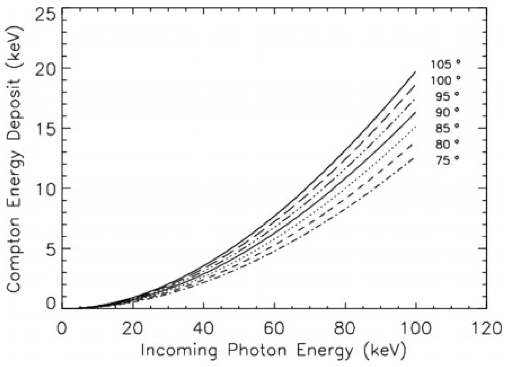
Given that the polarimeter is designed to accept mostly photons scattered at angles around 90°, it is interesting to see the energies involved. The energy given to an electron in the scatterer is
This is the second distribution driving the design. In all cases of interest for the discussion, this energy given to the electron is at maximum of a few tens of keV. With solid detectors, it can be assumed that it is converted in ionization or excitation within a few microns.
4. Practical Implementations
In this paper, I only discuss scattering polarimeters sensitive in the hard X-ray band, namely at energies > 15 keV, where the scattering is no more overwhelmed by photoabsorption and <150 keV, not to enter in the -ray range. From the equation, this corresponds to a few tens of keV at the high-energy side and to a few keV (or even a fraction of keV) at the low-energy side. I cannot conduct a systematic discussion of all possible configurations or their combination. Therefore, I select some examples of actually implemented instruments or of instruments with an adequate level of study.
The Materials Involved
In a two-phase polarimeter, the scatterer is always a material of low atomic number and of reasonable density (no gas). Lithium and Beryllium are used for passive scattering polarimeters, as well as a plastic scintillator for active scattering polarimeters. Lithium Hydride is, in theory, the best material (lowest Z, denser than Lithium), but it has some instabilities that discourage its use. In any case, both Lithium and Lithium Hydride are hygroscopic and must be encased in a thin Beryllium container. Therefore, some Beryllium is present in any case. In Table 1, the materials used in practice are shown.
One-phase polarimeters are (of course) only active. The material must be suitable as a detector. The two basic design include arrays of plastic scintillator and arrays of medium-atomic-number scintillators, such as Tallium activated Cesium Iodide (CsI) or Cerium activated Gadolinium Aluminium Gallium Garnet (GAGG).
5. Without Optics
5.1. Passive Scatterer
Following an historical sequence, the first implementation was conducted by the Columbia Team lead by Robert Novick. The payload was a set of Lithium blocks surrounded by proportional counters. The blocks were aligned with the rocket spinning axis pointed to the source [14,15]. This was, in fact, the very first attempt to perform X-ray polarimetry, and the first of a long sequence of upper limits. The second time, a stage based on Bragg crystals was added to the rocket payload, and from this combination, the first positive detection arrived [15]. The experience of rockets showed that the scattering technique in this implementation was much less sensitive than Bragg, so it was abandoned in the rocket age and in the early satellite age.
Many years later, a little block of Beryllium was set in between some Germanium detectors of the RHESSI mission. The band arrived to low energies (20 keV) due to the use of Be as a scatterer (typical two-phase polarimeter). A certain protection from the high background of direct unscattered photons was achieved with the capability to identify photons absorbed in the lower part of Germanium detectors, so that the upper part acted in practice as a shield [16].
But the results for RHESSI as a polarimeter were modest, basically upper limits, and still confirmed the mismatching of sensitivity of a polarimeter with the other instruments and the consequent poor throughput from what I named a byproduct polarimeter.
Only a dedicated satellite can effectively apply this technique. The POLIX instrument includes a collimator, aligned with the spin axis, a Beryllium scatterer in a well, of four proportional counters, heritage of ASTROSAT. POLIX is hosted aboard the XPoSAT mission by ISRO that was launched on 1 January 2024. The nominal range is 8–30 keV. POLIX [17] is mainly aimed to study bright sources on the basis of pointing of the order of a few weeks, possible with a dedicated satellite.
5.2. Active Scatterer
A polarimeter can be conceived as a combination of detectors. For known sources, a collimator limits the direction of primary photons, while only a large field delimiter is used for bursts. The temporal coincidence identifies the path of the scattered photon from the scatterer to the final absorber. The sum of the two detected energies is the total energy. For tens of years (as in [18,19]), this was merely conceptual. The straightforward implementation is with a low-atomic-number detector as a scatterer and a higher-atomic-number detector as an absorber. Typical pairs are a plastic scintillator and an CsI. Many different configurations have been proposed. The New Hampshire University Team has a long record of proposed and prototypized payloads. The Gamma-Ray polarimeter experiment (GRAPE) based on an array of bars of plastic scintillators surrounded by bars of CsI, read with a multi-anode photomultiplier, was tested aboard balloon flights. With a collimator, it can be used to measure known sources; without a collimator, it can study GRBs. A more recent version uses Si PMTs instead of MAPMTs. A version with seven moduli named a Large Area Burst Polarimeter (LEAP) should be the first such polarimeter to proceed on orbit aboard the ISS [20].
A small experiment for Gamma-Ray Bursts was IKAROS-GAP [21]. It was a single block of a plastic scintillator, surrounded with 12 CsI detectors with individual photomultipliers acting as absorbers. This was a raw and effective design but robust and well calibrated.
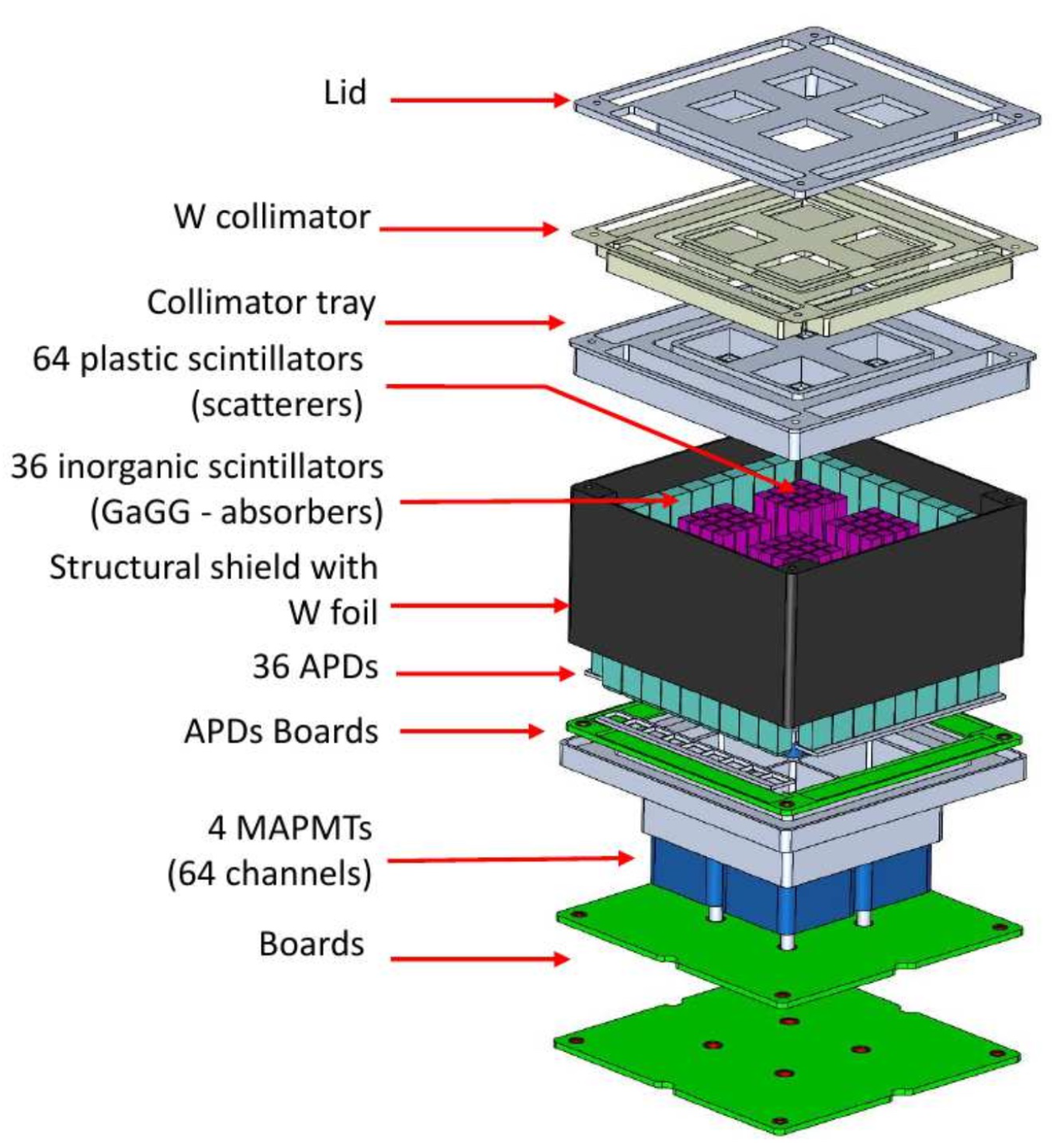
A mission in progress based on the concept of an active scatterer is the CUbesat Solar Polarimeter (CUSP) [22] aimed to develop a constellation of two CubeSats to measure the linear polarisation of solar flares in the hard X-ray band, in progress at IAPS-INAF under the management of Italian Space Agency. The payload is based on an array of bars of a plastic scintillator, surrounded by bars of GAGG, which is faster than CsI. Plastic scintillators are read with four multi-anode photomultipliers, R7600, while the GAGG bars are read with avalanche photo-diodes as shown in Figure 3.
One-phase active scattering polarimeters using the same material for both functions are conceptually less performing. A good efficiency would be achieved with a high probability of scattering in the first detector and a high probability of absorption in the second. Since the two processes compete, this is not possible by definition. At low energies where the absorption is mainly photoelectric and thence fast depending on the energy, and where the energies of the two processes are very different (as clear from Figure 2), the scattering/absorption is very ineffective. Yet, there is the possibility of a first Compton interaction in a detector and a second Compton interaction in another detector. The probability of this second interaction, after scattering at angles around 90°, can be maximized with a an array of thin wire-like detectors of a large area. The process is also modulated with polarization. The difficulty is that the sum of the two energies lost is lesser than the energy of the incoming photon. The modulation factor depends on the energy, so if the energy of the photon is not known, the conversion from the modulation to the polarization is very ambiguous. In any case, these experiments by simulations and calibrations can produce the polarization on a broad band that is absolutely correct if the spectrum is available from an independent instrument or from another mission.
The best implementation of this concept, based on plastic–plastic scattering, are the balloon payloads of the POGO family [23]. POGO is conceived to observe known sources with a narrow field of view. This is achieved with a tight passive/active collimator and with a heavy anticoincidence shield. In fact, POGO is the only one achieving results on discrete sources in the hard X-ray range [24].
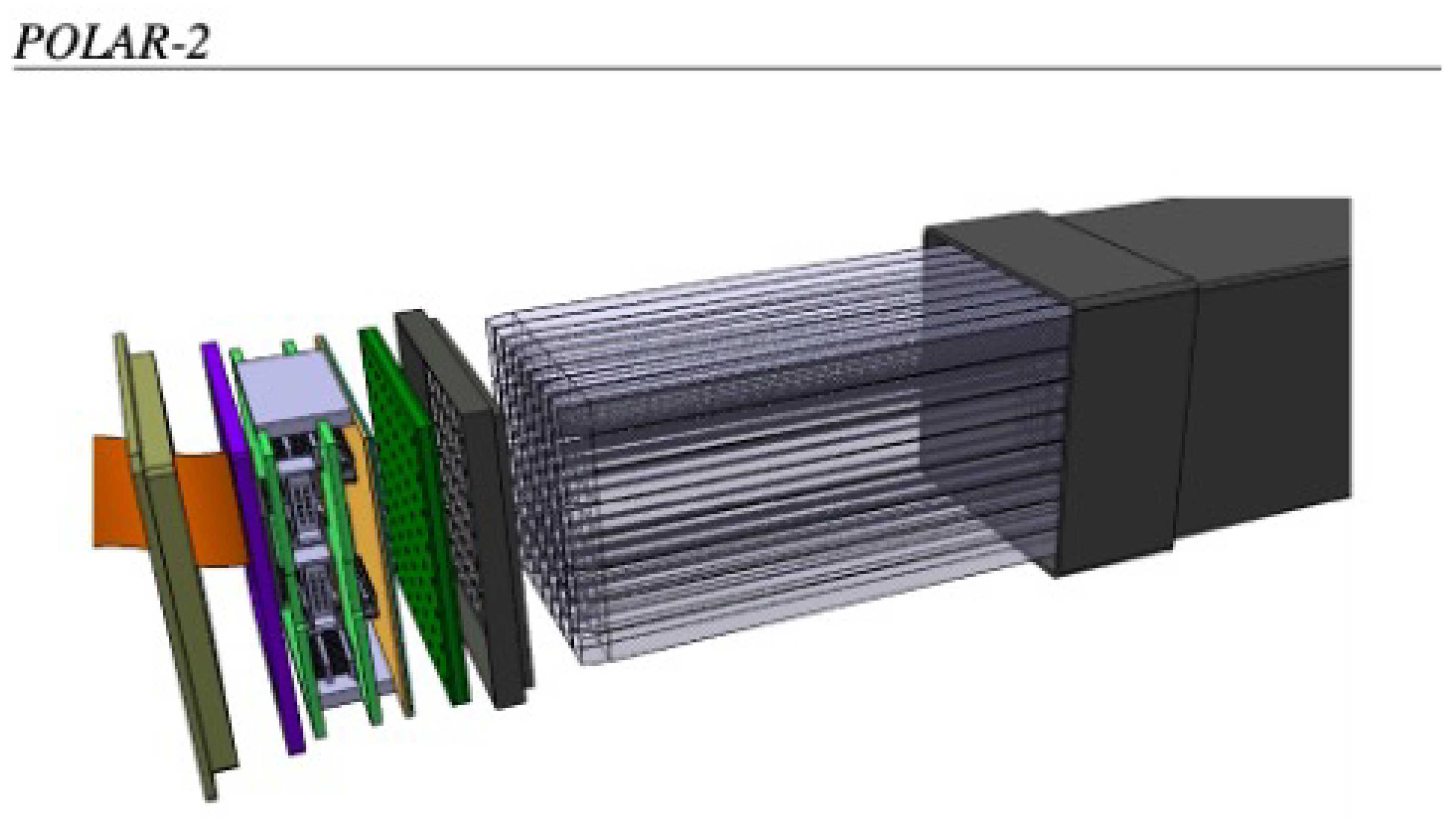
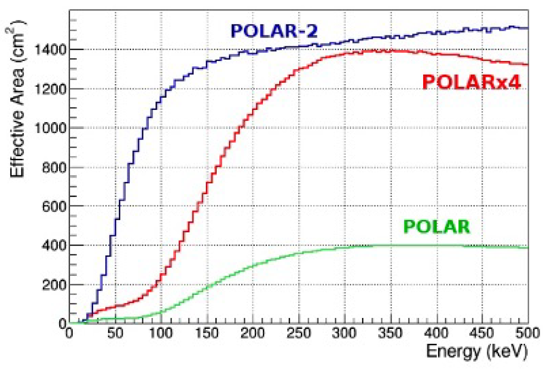
A strong argument in favor of the plastic–plastic configuration is the possibility of having large arrays of wire-like scintillators with fine subdivision using the same photonic device reading all the sensing units. This allows for a better use of space and makes everything simpler, from the alignment to the optical contacts to the readout electronics. The best implementation of this approach for a wide field instrument was POLAR [25,26], an array of plastic scintillator wires, read with a multi-anode photo multiplier. Flown aboard the Chinese space lab, POLAR was a very successful mission, the best for GRB polarimetry, but in a typical -ray band, marginal to our range of interest. But, POLAR-2, a new version in an advanced stage [27], will increase the area and use Silicon photo multipliers as in Figure 4. The lower energy threshold in POLAR-2 is somewhere between 20 and 30 keV, as shown in Figure 5, an interesting extension of the technique toward the X-ray band.
5.3. Byproduct Polarimetry
By byproduct polarimetry I mean instruments designed and built for some other purpose also conducting some polarimetry. Structured instruments sometimes include intermediate data that contain information on linear polarization. If these data are transmitted (by original design or by late additions), the instrument can be used as a polarimeter.
Given that polarization is more difficult to detect than spectra, images or timing of the technique usually apply to a very limited subset of the brightest sources.
Moreover, polarimetry requires an extreme (almost maniacal) care in the prevention of systematics that is absent in candidate byproduct polarimeters. In most cases, it does not work at all. The only substantial exception is ASTROSAT [28]. The Cadmium–Zinc–Telluride Imager (CZTI) is a hard X-ray coded mask camera working in the band of 10–100 keV. Pixels of CZT, 5 mm thick, have a reasonable fraction of Compton interactions at higher energies. Some of these scattered photons are absorbed by other pixels. Laboratory tests showed that the corrected angular distribution is modulated by polarization. One problem of such an approach is that the distribution is sensitive to the interaction point, and this can be very critical in a focal plane instrument. But, in the case of ASTROSAT, this is substantially mitigated with a parallel beam. Moreover, even though the instrument was calibrated as a polarimeter before the launch only on the axis [28,29], all the simulated response, including the dependence of this modulation on the offset angle, was verified with measurements performed on ground on a representative physical model [30,31]. So, in this case, we have the needed reliability, but, of course, the point that it only works with very strong sources holds.
6. In the Focal Plane
6.1. Optics in X-ray Astronomy and Optics in X-ray Polarimetry
The introduction of optics was the turning point in X-ray Astronomy as proposed by Riccardo Giacconi soon after the first discovery. With the mission Einstein in 1978, X-ray Astronomy achieved the capability to image extended sources [32]. But the major breakthrough was the capability to detect very weak sources because, with an imaging detector in the focus, the flux of the source is compared with the fluctuations of the background in the point spread function and not on the whole detector or one half of that (as in experiments with collimators or coded masks). The conventional polarimeters, based on Bragg diffraction, were totally mismatched in sensitivity with imagers and found no more place in multi-instrument missions. Since then, the the path to the polarimetry of known sources has been the quest for an imaging detector. This is based on photoelectric effect at low energies. But the technology of X-ray optics extends to hard X-rays due to multi-layer technology, and in this energy range, the viable process is scattering.
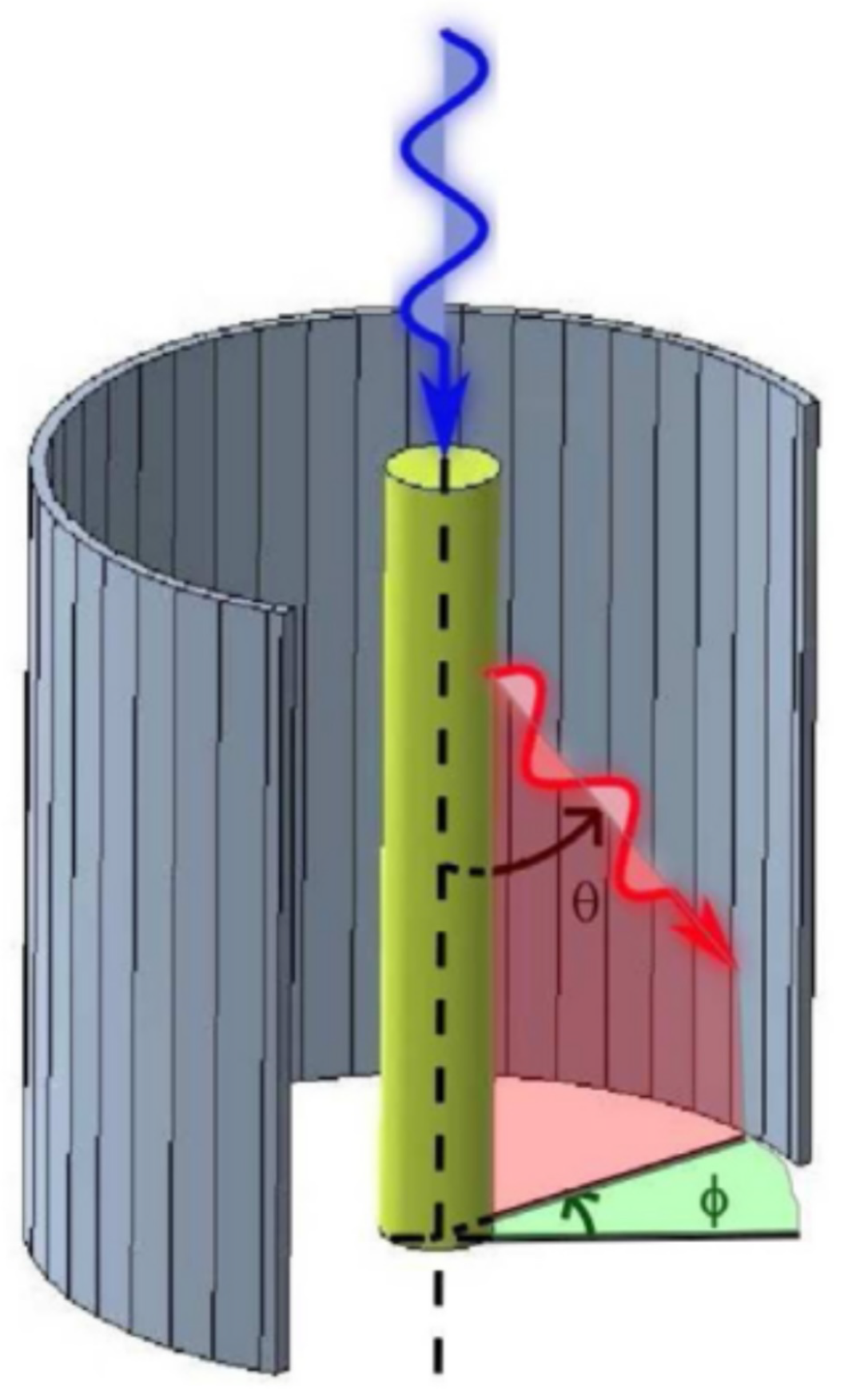
IXPE was possible because the Gas Pixel Detector allows for the reconstruction of the impact point of the photon and the angle of ejection of the photoelectron [2,33]. This means that to the counts from a point-like source background, counts are added from a surface of the order of 0.5 mm2, namely of less than 20 μCrab. In practice, the background has no impact on sensitivity for any point-like source when integrating on the 2–8 keV band. While IXPE has demonstrated that focal plane photoelectric polarimetry is viable, the equivalent for scattering has many criticalities, most of all the poor localization of the first interaction. Here, I discuss how these affect the concept and how they can be mitigated or overcome. Any focal plane scattering polarimeter is a scatterer centered on the focus or near it surrounded with detectors. The optimal design is a cylindrical scatterer long enough to provide a reasonable efficiency and large enough to include all the divergent beams from the telescope and any possible misalignment. In practice, the scatterer needs to have a length of several cm and a diameter of <1 cm. An ideal detector should be cylindrical itself as shown in Figure 6, but in practical implementations, major or minor deviations from this geometry were and are needed.
6.2. Passive Scatterer in Focus
The ambitious Spectrum X-Gamma (SRG) of the Soviet Union hosted two large telescopes manufactured in Denmark [34]. The focal plane of one of them hosted the Stellar X-ray Polarimetry (SXRP) lead by Robert Novick [35], with a contribution of Italian teams. At the focus there was a scatterer of Lithium, encased in Beryllium, surrounded with a well of four proportional counters. In order to compensate possible misalignment [36], the detectors were positioned relatively far from the scatterer, and this was larger than the convergence of the beam. SXRP was the first exploitation of the optics in polarimetry. Starting from an area of the optics of around 1000 cm2, the effective area of the polarimeter was around 50 cm2, still a considerable value. But the background rate, due to the large area of the detectors, ranged between one-fourth and one half of the rate from the Crab. Therefore, the advantage of being in the focal plane was effective only for a few bright sources; a step forward with respect to OSO-8 but not yet a breakthrough.
SXRP was built and tested until acceptance, but the SRG satellite was never completed and flown. The work of calibration and simulation [37], however, performed for SXRP was a good basis for the future proposals of X-ray polarimetry.
A straightforward consequence was that the system should be more compact than SXRP. But this would not be sufficient. In the interplay between efficiency and background, the first problem is the thickness of the scatterer. A lithium scatterer, to have reasonable efficiency, must have a length of more or less 10 cm. On the other hand, a system that is too long accepts photons scattered at large polar angles, which are poorly modulated. A scatterer of Beryllium could be long, about one-third but not less, given that at 30 keV, 3 cm of Be are transparent to 45% of photons. On the contrary, most of the decisions on modulation vs efficiency vs background trade-off, gives a larger value. The well of detectors must be as long as the scatterer. Also, a design tighter then SXRP has a radius of centimeters, and thence a surface of tens of square centimeters, nothing to do with p.s.f. of a fraction of a square millimeter of photoelectric low-energy detectors. The ratio of S/B in Equation (1) is not reduced at the same level. This is a simple truth, directly derived from cross-sections. A design achieving an optimal trade-off between the efficiency and the surface of the absorber will never escape to this. Moreover, in any detector, the instrumental background increases with energy. The realistic limit to the sample of targets available for these instruments is the flux for which the counts from the source are equal to those of the background. This limit can be lowered with a compact design and with techniques of background reduction. The best implementation of this concept, 20 years or more after SXRP, is the X-Calibur [38] mission and its evolution XL-Calibur [39], a scattering polarimeter in the focus of a multi-layer telescope onboard a stratospheric balloon, clearly also conceived as a pathfinder for a future satellite mission [40]. The X-Calibur telescope has a focal length of 8 m and an effective area of 93 cm2 at 20 keV. In the focus, a stick of Beryllium is the scatterer surrounded from a square well of CZT detectors acting as absorbers. The whole is surrounded with a CsI anticoincidence.
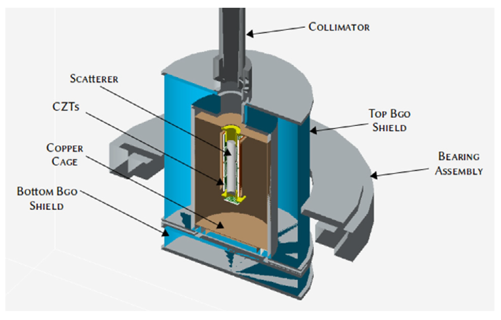
A flight from Antartica in 2018, with the observation of the bright source, GX301-2 [39], demonstrated the functionality of the whole but also showed the difficulty to achieve the real breakthrough with the introduction of optics only. The high background rate limited the sample of sources on which the measurement would be significant. This was mainly due to the limited efficiency (also due to the high zenith angle of bright sources at near-polar latitudes) and the high background (also maximum in polar regions). The analysis of this first flight drove the design of the evolved version of the experiment named XL-Calibur [41,42], also with the inclusion of the POGO team. The new focal plane set up is shown in Figure 7. The major improvements are as follows:
- A telescope with an increased collecting area (of 300 cm2 at 20 keV), also with a longer focal length of 12 m.
- An anticoincidence shield of BGO instead of CsI.
- Thinner detectors to reduce background.
The massive anticoincidence is somehow unavoidable since it is well known that in the hard X-ray range only active shielding with inorganic scintillators can drastically reduce the background.
With these improvements, the background rate in an arctic balloon should be of the order of 100 mCrab. Of course, a similar configuration aboard a satellite should be more sensitive because of higher efficiency, especially at lower energies.
6.3. Active Scatterer in the Focus
A way to overcome the problem of large background is to have an active scatterer, namely a detector in coincidence with the absorber. The rate of coincidences between the scatterer and the absorber should be much lower than the rate on the absorber only. But this has consequences in terms of efficiency. In order to understand whether this can be, in some cases, a viable solution, the materials involved should be discussed starting from Table 1. No detector exists based on Lithium or Beryllium. So the lowest (in practice, the only) useful materials are organic scintillators, where the scattering element is basically Carbonium. In terms of efficiency and background rate,
- The passive scatterer with Li has the lowest energy energy of transition from photo-absorption to scattering. With Be, the energy of transition is higher; higher still with an organic scintillator. The passive scatterer is more efficient also because of materials, and Lithium is better than Beryllium.
- With the active scatterer, the count rate from the source is lower than that with the passive scatterer with the same materials, because not every event of energy loss provides a signal suited to trigger the readout electronics and switch the coincidence.
In fact, the solution with the active scatterer was the original design of X-Calibur [40]. The scatterer was a stick of a plastic scintillator, 12 cm long, read with a photomultiplier. After a test flight, various measurements and simulations, it was found [38] that the reduction in the background of one order of magnitude was not adequate to compensate for the drastic drop of efficiency due, beside the aforementioned effect of materials, to the low coincidence trigger efficiency. So, eventually, X-Calibur and XL-Calibur went back to the passive scatterer design, which also benefitted from the larger density of Beryllium vs that of the plastic scintillator.
This choice was likely the best in the specific conditions but not necessarily the best for any case. In the literature, the performances of a scatterer of a plastic scintillator were studied at least twice [5,43], also with a certain number of tests. It is not clear how the background can be reduced, but it is evident that the crucial parameters are the overall efficiency and the trigger efficiency. The latter is a matter of energy but also of light collection. A passive scatterer can be made as long as possible, achieving an efficiency not far from one. In an active scatterer, the length is a trade-off to maximize the product of the interaction efficiency by the trigger efficiency and this for sure leads to a shorter scatterer. Both studies mentioned above show that the triggering efficiency increases with the energy of the incoming photon. With an increase in light collection efficiency, an active scattering solution should be more sensitive than a passive scatter one, at least above a certain energy that could range from 20 to 30 keV. Where exactly this occurs is not trivial. With a spectral slope of E−3, more than one half of the photons has 20 keV < E < 30 keV. With a passive scatterer, some photons of <20 keV can also be detected, but, for instance, in a balloon-borne instrument, the atmosphere absorbs most of photons of <30 keV.
Much depends on other factors. In an experiment like XL-Calibur, the design can be optimized on the basis of the instrument by itself. But if the polarimeter is combined with some other instrument peaked on a nearby band, the optimization will be performed for the combination of both, and the choice for the scattering stage can be different. In my opinion, if the photoelectric technique can be extended up to 20–25 keV, for the scattering stage, the active option becomes the best. This implies that the scatterer can be designed to maximize the sensitivity above 25 keV where the active scattering solution will be more effective.
7. The Path to the Future
From the IXPE experience and from the theoretical analysis, X-ray polarimetry is a technique of high scientific impact. This is true for all the three ranges and related detectors where Polarimetry is affordable, namely the low energy in the range of IXPE (2–10 keV), the medium energy still based on GPD with pressurized Argon filling (5–25 keV) [4,5,44] and the high energy based on scattering (20–80 keV). Moreover, the possibility to perform broad-band polarimetry is even more attractive.
A mission with three optics in parallel is possible; the possibility to stack two or more instruments is very useful, also allowing the presence of a telescope devoted to polarimetry and other telescopes pointing the same source to perform spectra and timing. In the past, instead of GPD, a Time Projection Chamber has been proposed for use for the low energies with a rear window of Beryllium, transparent to higher energy photons [44]. After this window, a scattering polarimeter active at high energies has also been hypothesized. The proposal is interesting and for sure can produce good measurements, but this configuration is not imaging in both stages and, after IXPE, giving up the possibility to study SuperNova Remnants, Pulsar Wind Nebulae, reflection clouds and Jets is difficult to accept. On the other hand, the GPD configuration with the drift field on the pointing direction unavoidably has the ASIC chip obstructing the path of higher-energy photons. One possibility with a potentially dramatic impact is to make the ASIC as thin as possible to leave a reasonable transparency to photons above 20 keV. In these chips, a thickness of 100 μm seems feasible and would guarantee the possibility to stack a LEP or a MEP with a scattering polarimeter in the rear.
Also, in a multi-telescope configuration, a combination of stacked instruments can be imaged to maximize the broad band throughput. In such a configuration, combination TPC/LEP - MEP - HEP stacked on the same telescope can be excellent for any point-like source, while the extended sources (Supernova remnants, Pulsar Wind Neblae, jets) of high interest but of limited number could be resolved with all the MEPs and with a single LEP in the imaging configuration. In my opinion, also in an active scattering configuration, a good anticoincidence is also useful for the MEP given that IXPE data also show that the background of photoelectric detectors seriously increases with energy. Last but not least, after achieving the necessary confidence, a Soft X-ray Telescope based on diffraction on a multi-layer with a laterally graded multi-layer component can enlarge the band to 0.15–0.30 keV as proposed, after more than 20 years of study, and described in Marshall (2018) [45].
Incidentally, I notice that a thin silicon device of ≤100 μm such as a Silicon Drift Detector (or, less likely given the high noise a Silicon Photomultiplier), substantially transparent to hard X-rays) can be used to read a cylinder of a scintillator from two sides with the two detectors in coincidence, drastically reducing the threshold and so increasing the trigger efficiency. It is a matter of fact that most of the thickness of these semiconductors is not hosting any electric component, but is needed as mechanical support or to make connections easier.
To conclude, a certain number of Research and Development activities can be the path to future missions of X-ray polarimetry extended to the hard X-ray band by the inclusion of one or more scattering stages.
- Feasibility of thinner ASIC pixel chips by testing the capability to support mechanical troubles and to allow connections.
- Feasibility of thinner photonic sensors to use two (or more) of them for the scatterer.
- Improving the radiation hardness of Si PMTs.
- Testing the windows of Silicon Nitride.
- Testing the triggering threshold of long plastic scintillators.
- Comparing the yield and the transparency of alternative organic scintillators (Anthracene, Stilbene, etc.).
- Following the progress of single-crystal diamond detectors that have been recently proposed as potential scatterers [46], although they are far from the needed performances.
- Simulation of the background in satellite orbits and potential anticoincidence materials.
The result of these studies could allow performance of experiments of polarimetry with the goal to achieve a more balanced sensitivity in terms of mCrab with a balanced combination of detectors in different bands.
Funding
This research received no external funding.
Data Availability Statement
No new data were created for this research.
Acknowledgments
This research could benefit of useful discussions with colleagues Ettore Del Monte, Sergio Fabiani, Fabio Muleri and Paolo Soffitta.
Conflicts of Interest
The author declares no conflict of interest.
References
- Costa, E. General History of X-ray Polarimetry in Astrophysics. In Handbook of X-ray and Gamma-ray Astrophysics; Springer-Nature: Berlin/Heidelberg, Germany, 2022; p. 36. [Google Scholar] [CrossRef]
- Costa, E.; Soffitta, P.; Bellazzini, R.; Brez, A.; Lumb, N.; Spandre, G. An efficient photoelectric X-ray polarimeter for the study of black holes and neutron stars. Nature 2001, 411, 662–665. [Google Scholar] [CrossRef]
- Zhang, S.; Santangelo, A.; Feroci, M.; Xu, Y.; Lu, F.; Chen, Y.; Feng, H.; Zhang, S.; Brandt, S.; Hernanz, M.; et al. The enhanced X-ray Timing and Polarimetry mission—eXTP. Sci. China Phys. Mech. Astron. 2019, 62, 29502. [Google Scholar] [CrossRef]
- Muleri, F.; Bellazzini, R.; Costa, E.; Soffitta, P.; Lazzarotto, F.; Feroci, M.; Pacciani, L.; Rubini, A.; Morelli, E.; Baldini, L.; et al. An X-ray polarimeter for hard X-ray optics. Proc. SPIE 2006, 6266, 62662X. [Google Scholar] [CrossRef]
- Fabiani, S.; Bellazzini, R.; Berrilli, F.; Brez, A.; Costa, E.; Minuti, M.; Muleri, F.; Pinchera, M.; Rubini, A.; Soffitta, P.; et al. Performance of an Ar-DME imaging photoelectric polarimeter. Proc. SPIE 2012, 8443, 84431C. [Google Scholar] [CrossRef]
- Chattopadhyay, T. Hard X-ray polarimetry—An overview of the method, science drivers, and recent findings. J. Astrophys. Astron. 2021, 42, 106. [Google Scholar] [CrossRef]
- Del Monte, E.; Fabiani, S.; Pearce, M. Compton Polarimetry. In Handbook of X-ray and Gamma-ray Astrophysics; Bambi, C., Santangelo, A., Eds.; Springer-Nature: Berlin/Heidelberg, Germany, 2023; p. 127. [Google Scholar] [CrossRef]
- McConnell, M.L. High energy polarimetry of prompt GRB emission. New Astron. Rev. 2017, 76, 1–21. [Google Scholar] [CrossRef]
- Weisskopf, M.C.; Elsner, R.F.; O’Dell, S.L. On understanding the figures of merit for detection and measurement of X-ray polarization. Proc. SPIE 2010, 7732, 77320E. [Google Scholar] [CrossRef]
- Strohmayer, T.E.; Kallman, T.R. On the Statistical Analysis of X-ray Polarization Measurements. Astrophys. J. 2013, 773, 103. [Google Scholar] [CrossRef]
- Muleri, F. Analysis of the Data from Photoelectric Gas Polarimeters. In Handbook of X-ray and Gamma-ray Astrophysics; Springer-Nature: Berline/Heidelberg, Germany, 2022; p. 6. [Google Scholar] [CrossRef]
- Fabiani, S.; Campana, R.; Costa, E.; Del Monte, E.; Muleri, F.; Rubini, A.; Soffitta, P. Characterization of scatterers for an active focal plane Compton polarimeter. Astropart. Phys. 2013, 44, 91–101. [Google Scholar] [CrossRef]
- McMaster, W.H. Matrix Representation of Polarization. Rev. Mod. Phys. 1961, 33, 8–27. [Google Scholar] [CrossRef]
- Angel, J.R.; Novick, R.; vanden Bout, P.; Wolff, R. Search for X-ray Polarization in Sco X-1. Phys. Rev. Lett. 1969, 22, 861–865. [Google Scholar] [CrossRef]
- Novick, R.; Weisskopf, M.C.; Berthelsdorf, R.; Linke, R.; Wolff, R.S. Detection of X-ray Polarization of the Crab Nebula. Astrophys. J. 1972, 174, L1. [Google Scholar] [CrossRef]
- McConnell, M.L.; Ryan, J.M.; Smith, D.M.; Lin, R.P.; Emslie, A.G. RHESSI as a Hard X-ray Polarimeter. Sol. Phys. 2002, 210, 125–142. [Google Scholar] [CrossRef]
- Paul, B.; Gopala Krishna, M.R.; Puthiya Veetil, R. POLIX: A Thomson X-ray polarimeter for a small satellite mission. In Proceedings of the 41st COSPAR Scientific Assembly, Istanbul, Turkey, 30 July–7 August 2016; Volume 41. Abstract id E1.15-8-16. [Google Scholar]
- McConnell, M.; Forrest, D.; Levenson, K.; Vestrand, W.T. The design of a gamma-ray burst polarimeter. In AIP Conference Proceedings, Proceedings of the Compton Gamma-ray Observatory, St. Louis, MO, USA, 15–17 October 1992; American Institute of Physics Conference Series; Friedlander, M., Gehrels, N., Macomb, D.J., Eds.; AIP: Kentwood, MI, USA, 1993; Volume 280, pp. 1142–1146. [Google Scholar] [CrossRef]
- Costa, E.; Cinti, M.N.; Feroci, M.; Matt, G.; Rapisarda, M. Design of a scattering polarimeter for hard X-ray astronomy. Nucl. Instrum. Methods Phys. Res. A 1995, 366, 161–172. [Google Scholar] [CrossRef]
- McConnell, M.L.; Baring, M.; Bloser, P.; Briggs, M.S.; Ertley, C.; Fletcher, G.; Gaskin, J.; Gelmis, K.; Goldstein, A.; Grove, E.; et al. The LargE Area burst Polarimeter (LEAP) a NASA mission of opportunity for the ISS. Proc. SPIE 2021, 11821, 118210P. [Google Scholar] [CrossRef]
- Yonetoku, D.; Murakami, T.; Gunji, S.; Mihara, T.; Sakashita, T.; Morihara, Y.; Kikuchi, Y.; Takahashi, T.; Fujimoto, H.; Toukairin, N.; et al. Gamma-Ray Burst Polarimeter (GAP) aboard the Small Solar Power Sail Demonstrator IKAROS. Publ. Astron. Soc. Jpn. 2011, 63, 625–638. [Google Scholar] [CrossRef]
- Fabiani, S.; Baffo, I.; Bonomo, S.; Contini, G.; Costa, E.; Cucinella, G.; De Cesare, G.; Del Monte, E.; Del Re, A.; Di Cosimo, S.; et al. CUSP: A two CubeSats constellation for space weather and solar flares X-ray polarimetry. Proc. SPIE 2022, 12181, 121810J. [Google Scholar] [CrossRef]
- Friis, M.; Kiss, M.; Mikhalev, V.; Pearce, M.; Takahashi, H. The PoGO+ Balloon-Borne Hard X-ray Polarimetry Mission. Galaxies 2018, 6, 30. [Google Scholar] [CrossRef]
- Chauvin, M.; Florén, H.G.; Friis, M.; Jackson, M.; Kamae, T.; Kataoka, J.; Kawano, T.; Kiss, M.; Mikhalev, V.; Mizuno, T.; et al. Shedding new light on the Crab with polarized X-rays. Sci. Rep. 2017, 7, 7816. [Google Scholar] [CrossRef]
- Produit, N.; Bao, T.W.; Batsch, T.; Bernasconi, T.; Britvich, I.; Cadoux, F.; Cernuda, I.; Chai, J.Y.; Dong, Y.W.; Gauvin, N.; et al. Design and construction of the POLAR detector. Nucl. Instrum. Methods Phys. Res. A 2018, 877, 259–268. [Google Scholar] [CrossRef]
- Suarez-Garcia, E.; Haas, D.; Hajdas, W.; Lamanna, G.; Lechanoine-Leluc, C.; Marcinkowski, R.; Mtchedlishvili, A.; Orsi, S.; Pohl, M.; Produit, N.; et al. A method to localize gamma-ray bursts using POLAR. Nucl. Instrum. Methods Phys. Res. A 2010, 624, 624–634. [Google Scholar] [CrossRef]
- Kole, M. POLAR-2: The First Large Scale Gamma-ray Polarimeter. In Proceedings of the 36th International Cosmic Ray Conference (ICRC2019), Madison, WI, USA, 24 July–1 August 2019; Volume 36, p. 572. [Google Scholar] [CrossRef]
- Vadawale, S.V.; Chattopadhyay, T.; Rao, A.R.; Bhattacharya, D.; Bhalerao, V.B.; Vagshette, N.; Pawar, P.; Sreekumar, S. Hard X-ray polarimetry with Astrosat-CZTI. Astron. Astrophys. 2015, 578, A73. [Google Scholar] [CrossRef]
- Chattopadhyay, T.; Vadawale, S.V.; Rao, A.R.; Sreekumar, S.; Bhattacharya, D. Prospects of hard X-ray polarimetry with Astrosat-CZTI. Exp. Astron. 2014, 37, 555–577. [Google Scholar] [CrossRef]
- Chattopadhyay, T.; Gupta, S.; Iyyani, S.; Saraogi, D.; Sharma, V.; Tsvetkova, A.; Ratheesh, A.; Gupta, R.; Mithun, N.P.S.; Vaishnava, C.S.; et al. Hard X-ray Polarization Catalog for a Five-year Sample of Gamma-Ray Bursts Using AstroSat CZT Imager. Astrophys. J. 2022, 936, 12. [Google Scholar] [CrossRef]
- Vaishnava, C.S.; Mithun, N.P.S.; Vadawale, S.V.; Aarthy, E.; Patel, A.R.; Adalja, H.L.; Kumar Tiwari, N.; Ladiya, T.; Navale, N.; Chattopadhyay, T.; et al. Experimental verification of off-axis polarimetry with cadmium zinc telluride detectors of AstroSat-CZT Imager. J. Astron. Telesc. Instrum. Syst. 2022, 8, 038005. [Google Scholar] [CrossRef]
- Giacconi, R.; Branduardi, G.; Briel, U.; Epstein, A.; Fabricant, D.; Feigelson, E.; Forman, W.; Gorenstein, P.; Grindlay, J.; Gursky, H.; et al. The Einstein (HEAO 2) X-ray Observatory. Astrophys. J. 1979, 230, 540–550. [Google Scholar] [CrossRef]
- Baldini, L.; Barbanera, M.; Bellazzini, R.; Bonino, R.; Borotto, F.; Brez, A.; Caporale, C.; Cardelli, C.; Castellano, S.; Ceccanti, M.; et al. Design, construction, and test of the Gas Pixel Detectors for the IXPE mission. Astropart. Phys. 2021, 133, 102628. [Google Scholar] [CrossRef]
- Schnopper, H.W. SODART telescopes on the Spectrum X-Gamma (SRG) and their complement of instruments. Proc. SPIE 1994, 2279, 412–423. [Google Scholar] [CrossRef]
- Kaaret, P.; Novick, R.; Martin, C.; Hamilton, T.; Sunyaev, R.; Lapshov, I.; Silver, E.; Weisskopf, M.; Elsner, R.; Chanan, G.; et al. SXRP. A focal plane stellar X-ray polarimeter for the SPECTRUM-X-Gamma mission. Proc. SPIE 1989, 1160, 587–597. [Google Scholar]
- Soffitta, P.; Costa, E.; Kaaret, P.; Dwyer, J.; Ford, E.; Tomsick, J.; Novick, R.; Nenonen, S. Proportional counters for the stellar X-ray polarimeter with a wedge and strip cathode pattern readout system. Nucl. Instrum. Methods Phys. Res. A 1998, 414, 218–232. [Google Scholar] [CrossRef]
- Kaaret, P.E.; Schwartz, J.; Soffitta, P.; Dwyer, J.; Shaw, P.S.; Hanany, S.; Novick, R.; Sunyaev, R.; Lapshov, I.Y.; Silver, E.H.; et al. Status of the stellar X-ray polarimeter for the Spectrum-X-Gamma mission. Proc. SPIE 1994, 2010, 22–27. [Google Scholar]
- Kislat, F.; Abarr, Q.; Beheshtipour, B.; De Geronimo, G.; Dowkontt, P.; Tang, J.; Krawczynski, H. Optimization of the design of X-Calibur for a long-duration balloon flight and results from a one-day test flight. J. Astron. Telesc. Instrum. Syst. 2018, 4, 011004. [Google Scholar] [CrossRef]
- Abarr, Q.; Baring, M.; Beheshtipour, B.; Beilicke, M.; de Geronimo, G.; Dowkontt, P.; Errando, M.; Guarino, V.; Iyer, N.; Kislat, F.; et al. Observations of a GX 301-2 Apastron Flare with the X-Calibur Hard X-ray Polarimeter Supported by NICER, the Swift XRT and BAT, and Fermi GBM. Astrophys. J. 2020, 891, 70. [Google Scholar] [CrossRef]
- Beilicke, M.; Baring, M.G.; Barthelmy, S.; Binns, W.R.; Buckley, J.; Cowsik, R.; Dowkontt, P.; Garson, A.; Guo, Q.; Haba, Y.; et al. Design and tests of the hard X-ray polarimeter X-Calibur. Nucl. Instrum. Methods Phys. Res. A 2012, 692, 283–284. [Google Scholar] [CrossRef]
- Abarr, Q.; Awaki, H.; Baring, M.G.; Bose, R.; De Geronimo, G.; Dowkontt, P.; Errando, M.; Guarino, V.; Hattori, K.; Hayashida, K.; et al. XL-Calibur—A second-generation balloon-borne hard X-ray polarimetry mission. Astropart. Phys. 2021, 126, 102529. [Google Scholar] [CrossRef]
- Iyer, N.K.; Kiss, M.; Pearce, M.; Stana, T.A.; Awaki, H.; Bose, R.G.; Dasgupta, A.; De Geronimo, G.; Gau, E.; Hakamata, T.; et al. The design and performance of the XL-Calibur anticoincidence shield. Nucl. Instrum. Methods Phys. Res. A 2023, 1048, 167975. [Google Scholar] [CrossRef]
- Chattopadhyay, T.; Vadawale, S.V.; Goyal, S.K.; Mithun, N.P.S.; Patel, A.R.; Shukla, R.; Ladiya, T.; Shanmugam, M.; Patel, V.R.; Ubale, G.P. Development of a hard X-ray focal plane compton polarimeter: A compact polarimetric configuration with scintillators and Si photomultipliers. Exp. Astron. 2016, 41, 197–214. [Google Scholar] [CrossRef]
- Jahoda, K.; Krawczynski, H.; Kislat, F.; Marshall, H.; Okajima, T. The X-ray Polarization Probe mission concept. Bull. Am. Astron. Soc. 2019, 51, 181. [Google Scholar]
- Marshall, H.L.; Günther, H.M.; Heilmann, R.K.; Schulz, N.S.; Egan, M.; Hellickson, T.; Heine, S.N.T.; Windt, D.L.; Gullikson, E.M.; Ramsey, B.; et al. Design of a broadband soft X-ray polarimeter. J. Astron. Telesc. Instrum. Syst. 2018, 4, 011005. [Google Scholar] [CrossRef]
- Poulson, D.; Bloser, P.F.; Ogasawara, K.; Lemire, C.R.; Trevino, J.A.; Legere, J.S.; Ryan, J.M.; McConnell, M.L. Using single-crystal diamond detectors as a scattering medium in Compton telescopes. Proc. SPIE 2022, 12181, 121812I. [Google Scholar] [CrossRef]
Figure 1.
Compton scattering has a high modulation around 90° decreasing to 0 for forward and backward scattering. From Fabiani (2013) [12].
Figure 1.
Compton scattering has a high modulation around 90° decreasing to 0 for forward and backward scattering. From Fabiani (2013) [12].

Figure 2.
The angles of scattering around 90° are those more interesting for polarimetry. Following Equation (4), the energy transferred to the scatterer can be computed as a function of the energy of the photon and of the scattering angle. From Fabiani (2013) [12].

Figure 3.
Exploded view of the CUSP payload. Photons from solar flares are scattered on the plastic scintillators and absorbed by GAGG scintillators. From Fabiani (2022) [22].
Figure 3.
Exploded view of the CUSP payload. Photons from solar flares are scattered on the plastic scintillators and absorbed by GAGG scintillators. From Fabiani (2022) [22].

Figure 4.
POLAR-2 is an assembly of moduli similar to POLAR but 4 times larger. The main difference is the use of Silicon Photomultipliers, allowing for a significant decrease in the threshold on the first interaction and, as a consequence, a very effective decrease in the low energy threshold of the whole. From Kole (2019) [27].

Figure 5.
POLAR-2 with respect of POLAR has a 4-fold larger area and a significantly lower threshold. From Kole (2019) [27].
Figure 5.
POLAR-2 with respect of POLAR has a 4-fold larger area and a significantly lower threshold. From Kole (2019) [27].

Figure 6.
A focal plane scattering polarimeter is always a cylindrical scatterer, centered on the axis and in the focal plane, surrounded with a well of detectors, ideally of cylindrical geometry. The scatterer can be a detector itself. In this case, it is named an Active Scatterer Focal Polarimeter. From Fabiani (2012) [5].

Figure 7.
The present configuration of the XL-Calibur focal plane instrument. The Beryllium scatterer is surrounded with four strings of CZT dtectors. All around, a thick BGO shield reduces the background. From Iyer (2023) [42].
Figure 7.
The present configuration of the XL-Calibur focal plane instrument. The Beryllium scatterer is surrounded with four strings of CZT dtectors. All around, a thick BGO shield reduces the background. From Iyer (2023) [42].


Table 1.
Materials used as a scatterer in a two-phase polarimeter. The third column displays the energy where the scattering equalizes absorption and in practice where the technique is fully operative. LiH, Li and Be are the favorites for passive scatterer configurations, while a plastic scintillator (or other organic scintillators) is the baseline as an active scatterer.
| Material | ρ (g · cm−3) | E (keV) Scatt = Absorption |
|---|---|---|
| Lithium | 0.53 | 8.7 |
| LiH | 0.82 | 8.2 |
| Beryllium | 1.85 | 14 |
| Plastc Scintillator (PVT) | 1.03 | 20 |
Disclaimer/Publisher’s Note: The statements, opinions and data contained in all publications are solely those of the individual author(s) and contributor(s) and not of MDPI and/or the editor(s). MDPI and/or the editor(s) disclaim responsibility for any injury to people or property resulting from any ideas, methods, instructions or products referred to in the content. |
© 2024 by the author. Licensee MDPI, Basel, Switzerland. This article is an open access article distributed under the terms and conditions of the Creative Commons Attribution (CC BY) license (https://creativecommons.org/licenses/by/4.0/).
Share and Cite
MDPI and ACS Style
Costa, E. Scattering Polarimetry in the Hard X-ray Range. Instruments 2024, 8, 20. https://doi.org/10.3390/instruments8010020
AMA Style
Costa E. Scattering Polarimetry in the Hard X-ray Range. Instruments. 2024; 8(1):20. https://doi.org/10.3390/instruments8010020
Chicago/Turabian StyleCosta, Enrico. 2024. "Scattering Polarimetry in the Hard X-ray Range" Instruments 8, no. 1: 20. https://doi.org/10.3390/instruments8010020