
Analysis of Near-Field Magnetic Responses on ZrTe5 through Cryogenic Magneto-THz Nano-Imaging
 , , , and
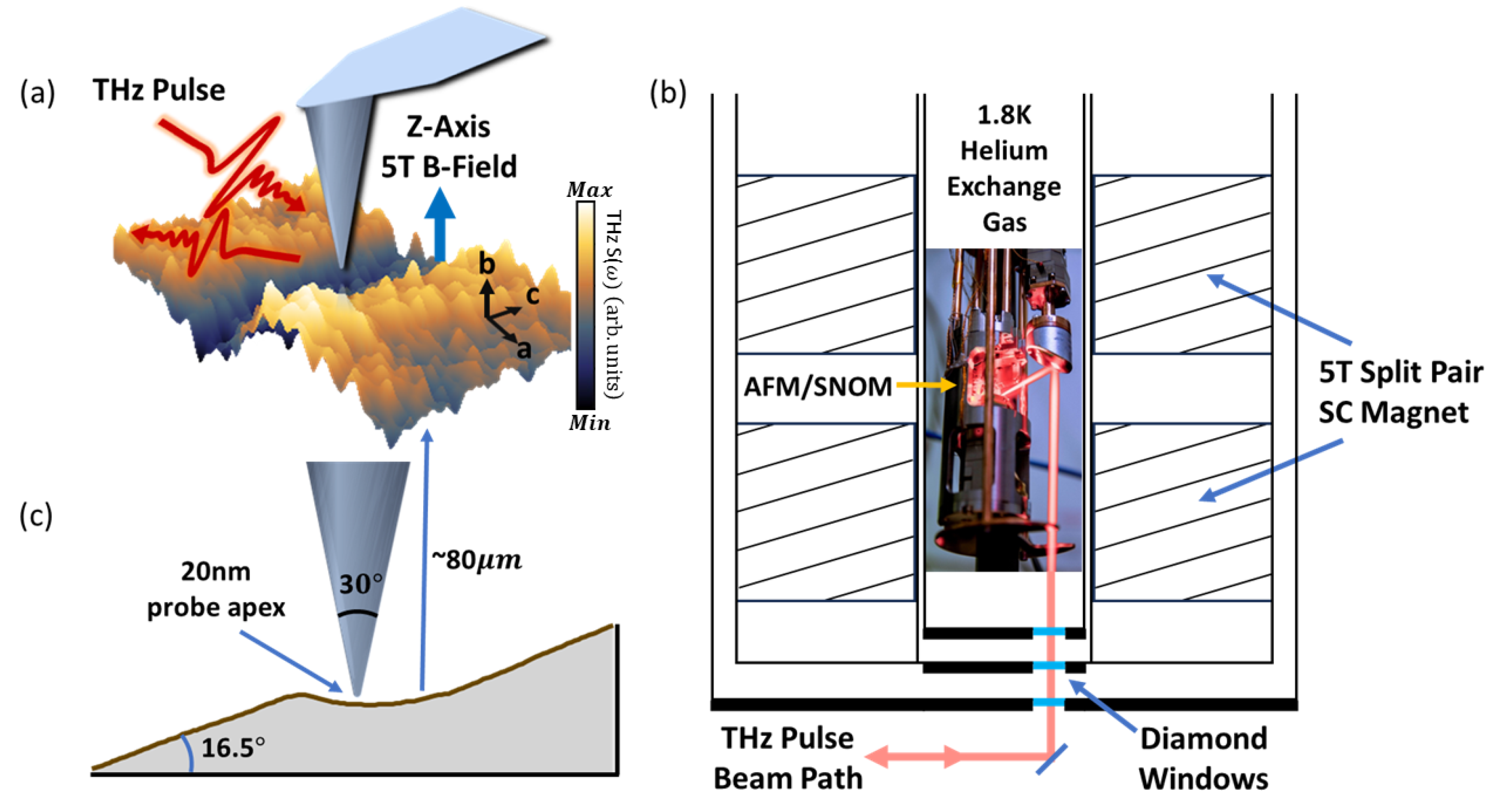
Abstract
:1. Introduction
2. Materials and Methods
3. Results and Analysis
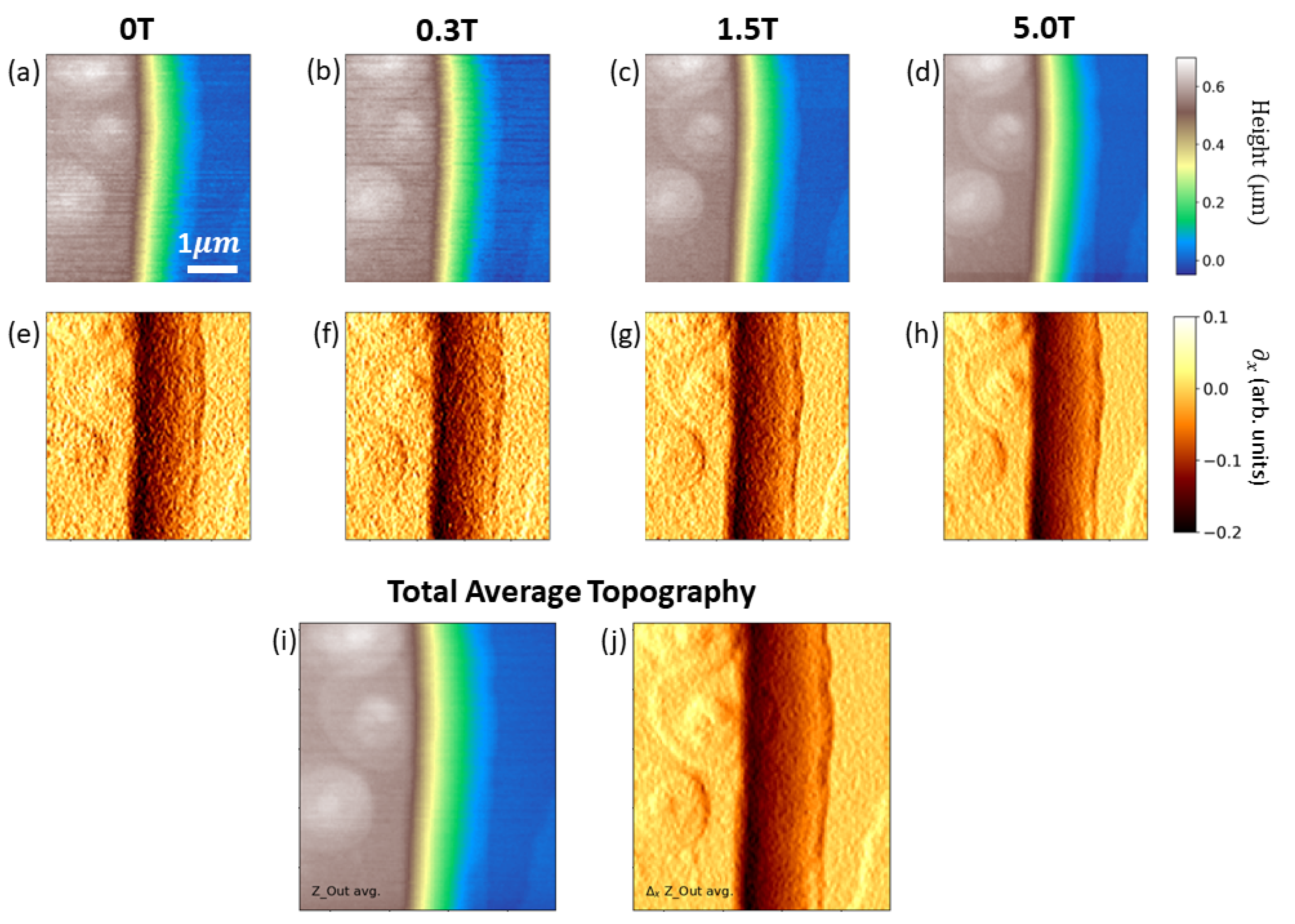
3.1. Methods of Analyzing Topography
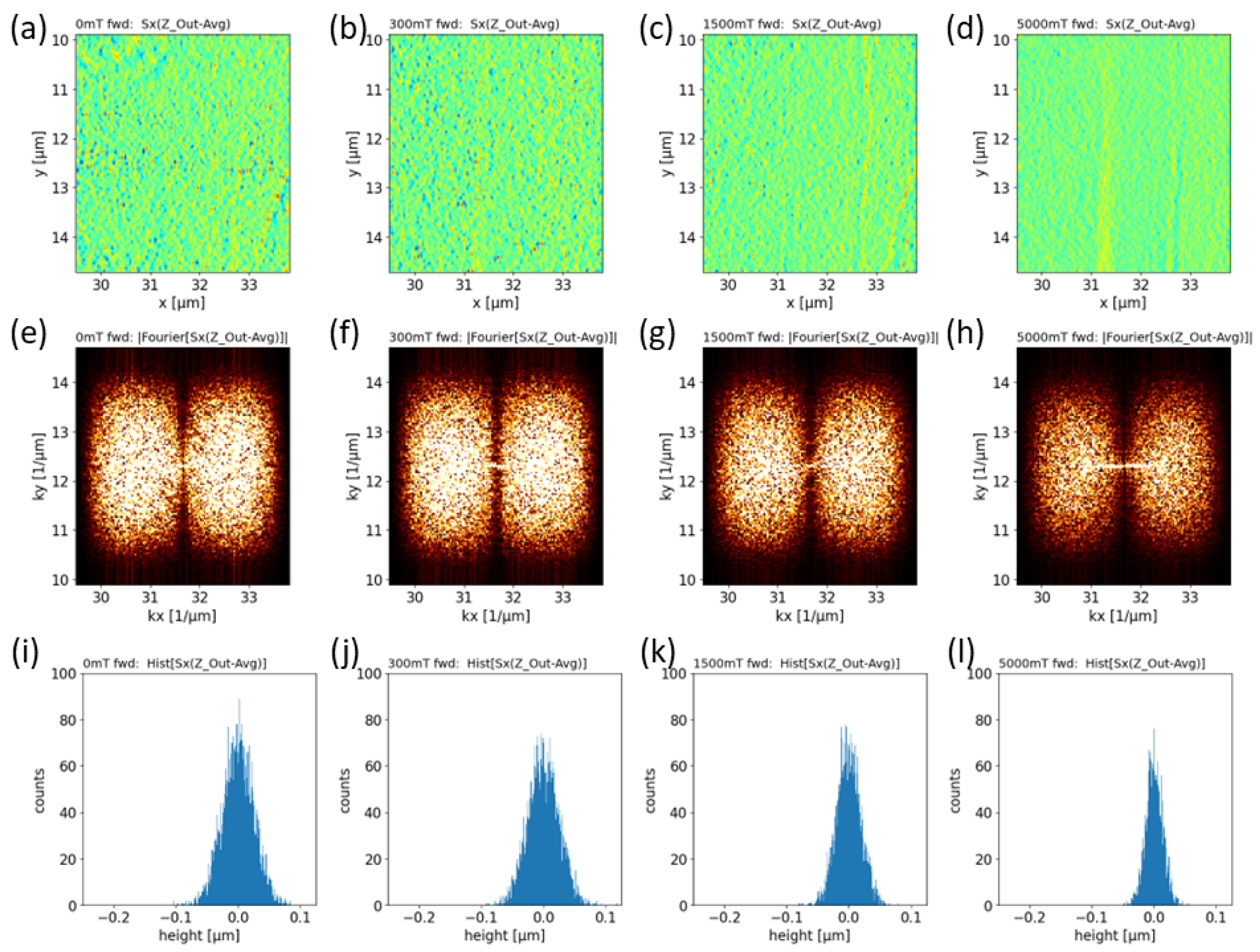
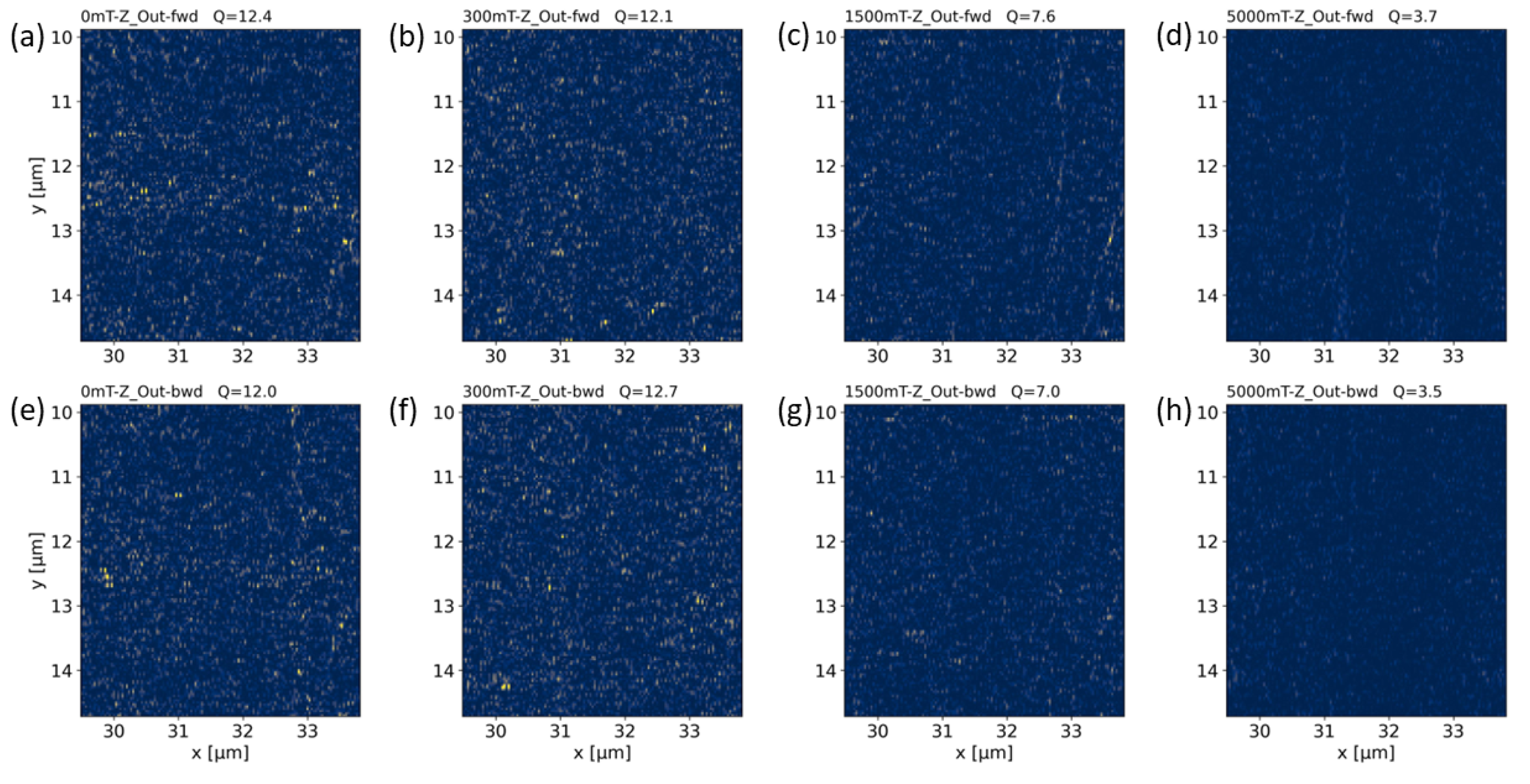
3.1.1. Detecting Fine Features and Edges Hidden by Large Topographic Variations—Sobel Operator
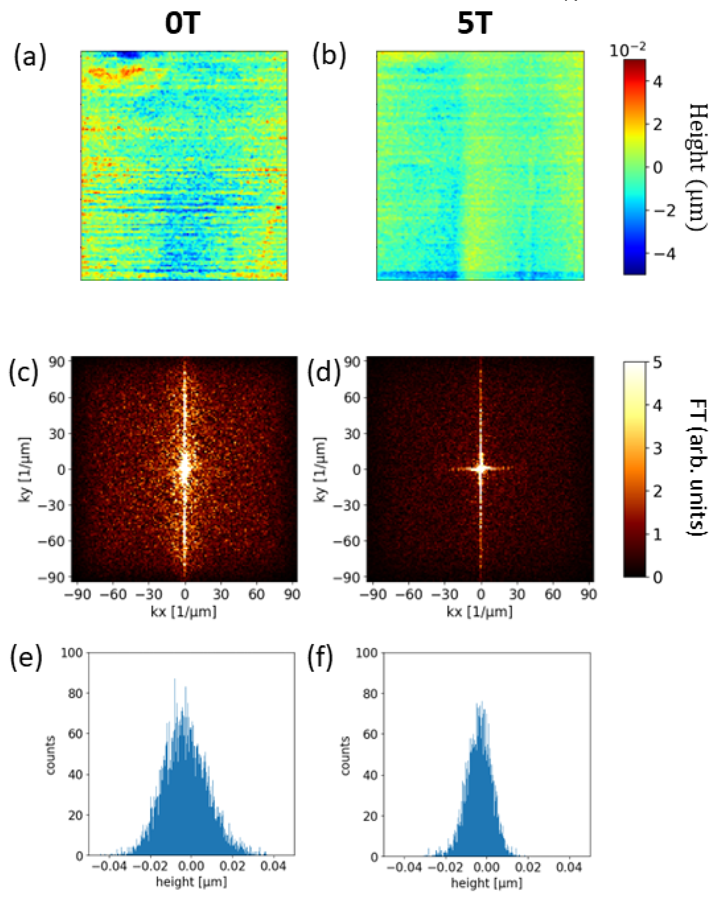
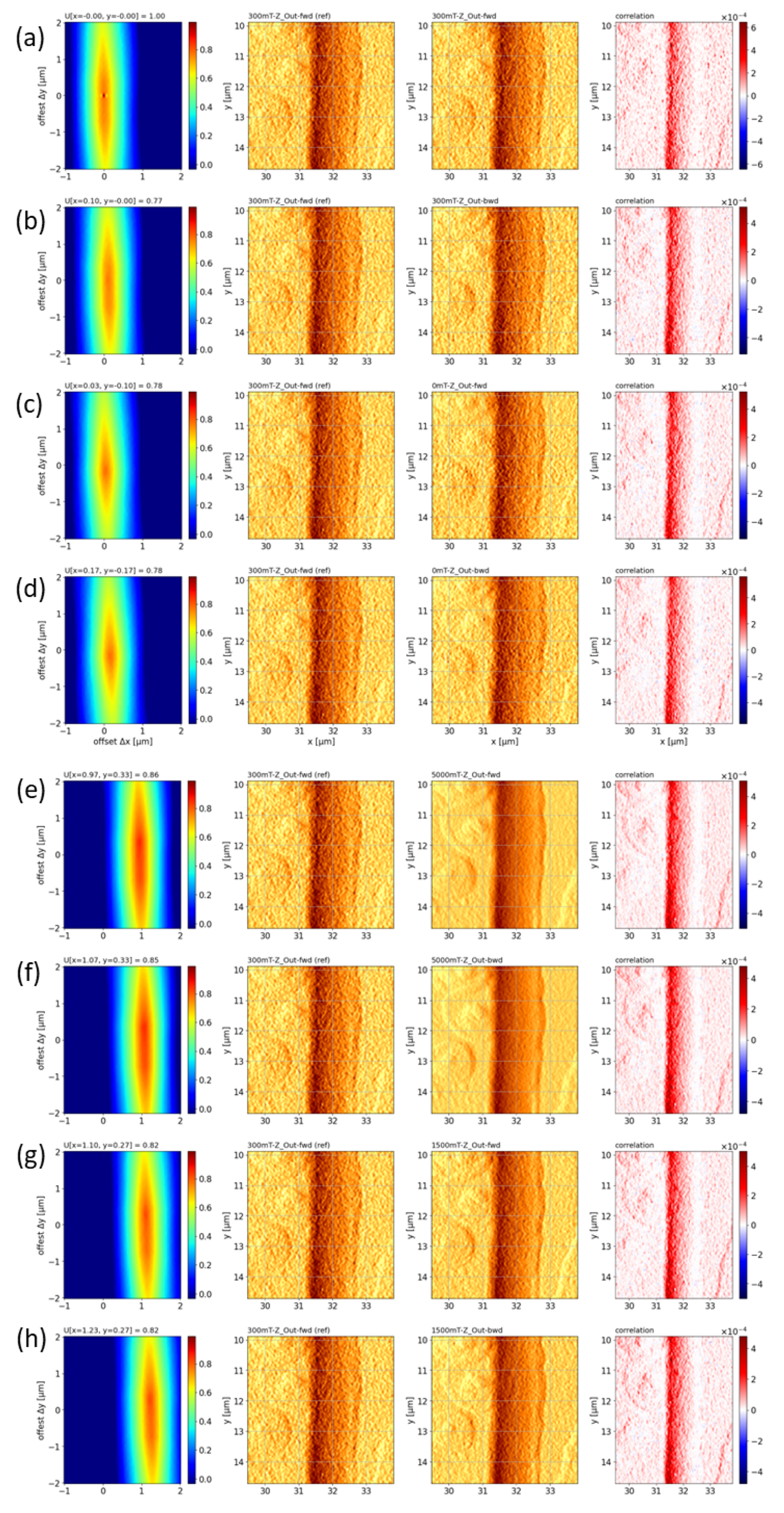
3.1.2. Correlating Topography under Different Conditions and “Noise-Free” Reference
3.1.3. Statistically Quantifying Magnetic Field Effects on AFM Operation
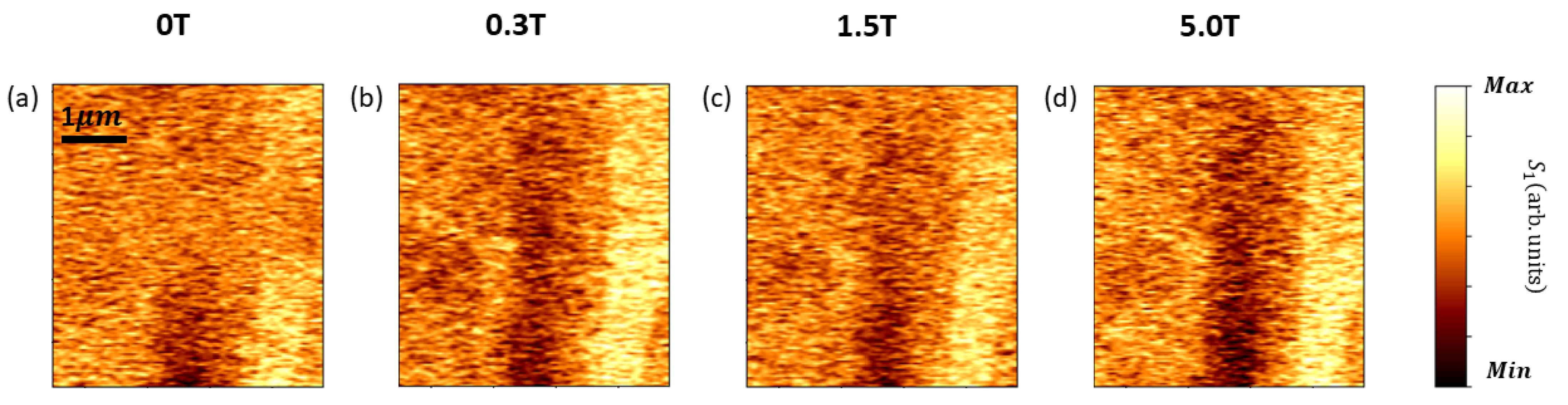
3.2. Deep Sub-Wavelength THz Near-Field imaging
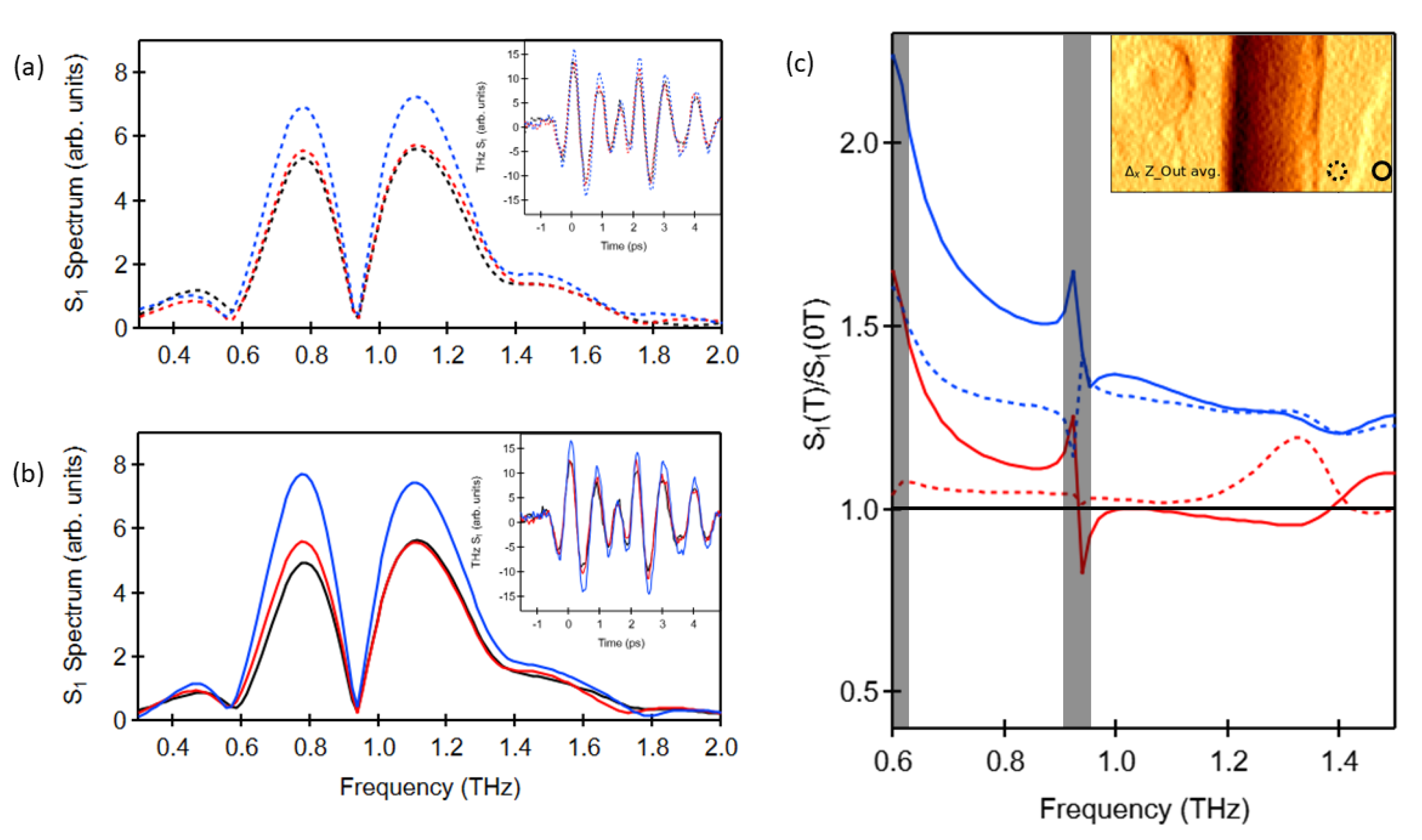
3.3. Deep Sub-Wavelength THz Time-Domain Spectroscopy
4. Conclusions
Author Contributions
Funding
Data Availability Statement
Acknowledgments
Conflicts of Interest
Appendix A


References
- Luo, L.; Mootz, M.; Kang, J.H.; Huang, C.; Eom, K.; Lee, J.W.; Vaswani, C.; Collantes, Y.G.; Hellstrom, E.E.; Perakis, I.E.; et al. Quantum Coherence Tomography of Light–Controlled Superconductivity. Nat. Phys. 2023, 19, 201–209. [Google Scholar] [CrossRef]
- Luo, L.; Yang, X.; Liu, X.; Liu, Z.; Vaswani, C.; Cheng, D.; Mootz, M.; Zhao, X.; Yao, Y.; Wang, C.Z.; et al. Ultrafast manipulation of topologically enhanced surface transport driven by mid-infrared and terahertz pulses in Bi2Se3. Nat. Commun. 2019, 10, 607. [Google Scholar] [CrossRef] [PubMed]
- Luo, L.; Cheng, D.; Song, B.; Wang, L.L.; Vaswani, C.; Lozano, P.M.; Gu, G.; Huang, C.; Kim, R.H.J.; Liu, Z.; et al. A light-induced phononic symmetry switch and giant dissipationless topological photocurrent in ZrTe5. Nat. Mater. 2021, 20, 329–334. [Google Scholar] [CrossRef] [PubMed]
- Arnold, F.; Shekhar, C.; Wu, S.C.; Sun, Y.; Dos Reis, R.D.; Kumar, N.; Naumann, M.; Ajeesh, M.O.; Schmidt, M.; Grushin, A.G.; et al. Negative magnetoresistance without well-defined chirality in the Weyl semimetal TaP. Nat. Commun. 2016, 7, 11615. [Google Scholar] [CrossRef] [PubMed]
- Liang, S.; Lin, J.; Kushwaha, S.; Xing, J.; Ni, N.; Cava, R.J.; Ong, N.P. Experimental tests of the chiral anomaly magnetoresistance in the Dirac-Weyl semimetals Na3Bi and GdPtBi. Phys. Rev. X 2018, 8, 031002. [Google Scholar] [CrossRef]
- Levy, A.L.; Sushkov, A.B.; Liu, F.; Shen, B.; Ni, N.; Drew, H.D.; Jenkins, G.S. Optical evidence of the chiral magnetic anomaly in the Weyl semimetal TaAs. Phys. Rev. B 2020, 101, 125102. [Google Scholar] [CrossRef]
- Jadidi, M.M.; Kargarian, M.; Mittendorff, M.; Aytac, Y.; Shen, B.; König-Otto, J.C.; Winnerl, S.; Ni, N.; Gaeta, A.L.; Murphy, T.E.; et al. Nonlinear optical control of chiral charge pumping in a topological Weyl semimetal. Phys. Rev. B 2020, 102, 245123. [Google Scholar] [CrossRef]
- Yuan, X.; Zhang, C.; Zhang, Y.; Yan, Z.; Lyu, T.; Zhang, M.; Li, Z.; Song, C.; Zhao, M.; Leng, P.; et al. The discovery of dynamic chiral anomaly in a Weyl semimetal NbAs. Nat. Commun. 2020, 11, 1259. [Google Scholar] [CrossRef]
- Stinson, H.T.; Sternbach, A.; Najera, O.; Jing, R.; Mcleod, A.S.; Slusar, T.V.; Mueller, A.; Anderegg, L.; Kim, H.T.; Rozenberg, M.; et al. Imaging the nanoscale phase separation in vanadium dioxide thin films at terahertz frequencies. Nat. Commun. 2018, 9, 3604. [Google Scholar] [CrossRef]
- Cocker, T.L.; Peller, D.; Yu, P.; Repp, J.; Huber, R. Tracking the ultrafast motion of a single molecule by femtosecond orbital imaging. Nature 2016, 539, 263–267. [Google Scholar] [CrossRef]
- Wang, L.; Xia, Y.; Ho, W. Atomic-scale quantum sensing based on the ultrafast coherence of an H2 molecule in an STM cavity. Science 2022, 376, 401–405. [Google Scholar] [CrossRef] [PubMed]
- Chen, H.T.; Kersting, R.; Cho, G.C. Terahertz imaging with nanometer resolution. Appl. Phys. Lett. 2003, 83, 3009–3011. [Google Scholar] [CrossRef]
- Von Ribbeck, H.G.; Brehm, M.; Van der Weide, D.; Winnerl, S.; Drachenko, O.; Helm, M.; Keilmann, F. Spectroscopic THz near-field microscope. Opt. Express 2008, 16, 3430–3438. [Google Scholar] [CrossRef] [PubMed]
- Zhang, J.; Chen, X.; Mills, S.; Ciavatti, T.; Yao, Z.; Mescall, R.; Hu, H.; Semenenko, V.; Fei, Z.; Li, H.; et al. Terahertz Nanoimaging of Graphene. ACS Photonics 2018, 5, 2645–2651. [Google Scholar] [CrossRef]
- Aghamiri, N.A.; Huth, F.; Huber, A.J.; Fali, A.; Hillenbrand, R.; Abate, Y. Hyperspectral time-domain terahertz nano-imaging. Opt. Express 2019, 27, 24231–24242. [Google Scholar] [CrossRef] [PubMed]
- Moon, K.; Do, Y.; Park, H.; Kim, J.; Kang, H.; Lee, G.; Lim, J.H.; Kim, J.W.; Han, H. Computed terahertz near-field mapping of molecular resonances of lactose stereo-isomer impurities with sub-attomole sensitivity. Sci. Rep. 2019, 9, 16915. [Google Scholar] [CrossRef] [PubMed]
- Pizzuto, A.; Castro-Camus, E.; Wilson, W.; Choi, W.; Li, X.; Mittleman, D.M. Nonlocal Time-Resolved Terahertz Spectroscopy in the Near Field. ACS Photonics 2021, 8, 2904–2911. [Google Scholar] [CrossRef]
- Plankl, M.; Faria Junior, P.E.; Mooshammer, F.; Siday, T.; Zizlsperger, M.; Sandner, F.; Schiegl, F.; Maier, S.; Huber, M.A.; Gmitra, M.; et al. Subcycle contact-free nanoscopy of ultrafast interlayer transport in atomically thin heterostructures. Nat. Photonics 2021, 15, 594–600. [Google Scholar] [CrossRef]
- Kim, R.H.J.; Huang, C.; Luan, Y.; Wang, L.L.; Liu, Z.; Park, J.M.; Luo, L.; Lozano, P.M.; Gu, G.; Turan, D.; et al. Terahertz Nano-Imaging of Electronic Strip Heterogeneity in a Dirac Semimetal. ACS Photonics 2021, 8, 1873–1880. [Google Scholar] [CrossRef]
- Kim, R.H.J.; Pathak, A.K.; Park, J.M.; Imran, M.; Haeuser, S.; Fei, Z.; Mudryk, Y.; Koschny, T.; Wang, J. Nano-compositional imaging of the lanthanum silicide system at THz wavelengths. Optics Express 2023, 32, 2356–2363. [Google Scholar] [CrossRef]
- Kim, R.H.J.; Liu, Z.; Huang, C.; Park, J.M.; Haeuser, S.J.; Song, Z.; Yan, Y.; Yao, Y.; Luo, L.; Wang, J. Terahertz Nanoimaging of Perovskite Solar Cell Materials. ACS Photonics 2022, 9, 3550–3556. [Google Scholar] [CrossRef]
- Kim, R.H.J.; Park, J.M.; Haeuser, S.; Huang, C.; Cheng, D.; Koschny, T.; Oh, J.; Kopas, C.; Cansizoglu, H.; Yadavalli, K.; et al. Visualizing heterogeneous dipole fields by terahertz light coupling in individual nano-junctions. Commun. Phys. 2023, 6, 147. [Google Scholar] [CrossRef]
- Wehmeier, L.; Liu, M.; Park, S.; Jang, H.; Basov, D.; Homes, C.C.; Carr, G.L. Ultrabroadband Terahertz Near-Field Nanospectroscopy with a HgCdTe Detector. ACS Photonics 2023, 10, 4329–4339. [Google Scholar] [CrossRef] [PubMed]
- Taghinejad, M.; Xia, C.; Hrton, M.; Lee, K.T.; Kim, A.S.; Li, Q.; Guzelturk, B.; Kalousek, R.; Xu, F.; Cai, W.; et al. Determining hot-carrier transport dynamics from terahertz emission. Science 2023, 382, 299–305. [Google Scholar] [CrossRef] [PubMed]
- Yang, H.U.; Hebestreit, E.; Josberger, E.E.; Raschke, M.B. A cryogenic scattering-type scanning near-field optical microscope. Rev. Sci. Instrum. 2013, 84, 023701. [Google Scholar] [CrossRef] [PubMed]
- Ni, G.; McLeod, d.A.; Sun, Z.; Wang, L.; Xiong, L.; Post, K.; Sunku, S.; Jiang, B.Y.; Hone, J.; Dean, C.R.; et al. Fundamental limits to graphene plasmonics. Nature 2018, 557, 530–533. [Google Scholar] [CrossRef] [PubMed]
- Lin, K.T.; Komiyama, S.; Kim, S.; Kawamura, K.i.; Kajihara, Y. A high signal-to-noise ratio passive near-field microscope equipped with a helium-free cryostat. Rev. Sci. Instrum. 2017, 88, 013706. [Google Scholar] [CrossRef]
- Dapolito, M.; Chen, X.; Li, C.; Tsuneto, M.; Zhang, S.; Du, X.; Liu, M.; Gozar, A. Scattering-type scanning near-field optical microscopy with Akiyama piezo-probes. Appl. Phys. Lett. 2022, 120, 013104. [Google Scholar] [CrossRef]
- Zhao, W.; Li, H.; Xiao, X.; Jiang, Y.; Watanabe, K.; Taniguchi, T.; Zettl, A.; Wang, F. Nanoimaging of low-loss plasmonic waveguide modes in a graphene nanoribbon. Nano Lett. 2021, 21, 3106–3111. [Google Scholar] [CrossRef]
- Lu, Q.; Bollinger, A.T.; He, X.; Sundling, R.; Bozovic, I.; Gozar, A. Surface Josephson plasma waves in a high-temperature superconductor. Npj Quantum Mater. 2020, 5, 69. [Google Scholar] [CrossRef]
- Dapolito, M.; Tsuneto, M.; Zheng, W.; Wehmeier, L.; Xu, S.; Chen, X.; Sun, J.; Du, Z.; Shao, Y.; Jing, R.; et al. Infrared nano-imaging of Dirac magnetoexcitons in graphene. Nat. Nanotechnol. 2023, 18, 1409–1415. [Google Scholar] [CrossRef]
- Kim, R.H.J.; Park, J.M.; Haeuser, S.J.; Luo, L.; Wang, J. A sub-2 Kelvin cryogenic magneto-terahertz scattering-type scanning near-field optical microscope (cm-THz-sSNOM). Rev. Sci. Instrum. 2023, 94, 043702. [Google Scholar] [CrossRef] [PubMed]
- Vaswani, C.; Wang, L.L.; Mudiyanselage, D.H.; Li, Q.; Lozano, P.; Gu, G.; Cheng, D.; Song, B.; Luo, L.; Kim, R.H.; et al. Light-driven Raman coherence as a nonthermal route to ultrafast topology switching in a Dirac semimetal. Phys. Rev. X 2020, 10, 021013. [Google Scholar] [CrossRef]
- Chen, J.; Badioli, M.; Alonso-González, P.; Thongrattanasiri, S.; Huth, F.; Osmond, J.; Spasenović, M.; Centeno, A.; Pesquera, A.; Godignon, P.; et al. Optical nano-imaging of gate-tunable graphene plasmons. Nature 2012, 487, 77–81. [Google Scholar] [CrossRef] [PubMed]
- Weng, H.; Dai, X.; Fang, Z. Transition-metal pentatelluride ZrTe5 and HfTe5: A paradigm for large-gap quantum spin Hall insulators. Phys. Rev. X 2014, 4, 011002. [Google Scholar]
- Manzoni, G.; Gragnaniello, L.; Autès, G.; Kuhn, T.; Sterzi, A.; Cilento, F.; Zacchigna, M.; Enenkel, V.; Vobornik, I.; Barba, L.; et al. Evidence for a strong topological insulator phase in ZrTe5. Phys. Rev. Lett. 2016, 117, 237601. [Google Scholar] [CrossRef] [PubMed]
- Xu, B.; Zhao, L.; Marsik, P.; Sheveleva, E.; Lyzwa, F.; Dai, Y.; Chen, G.; Qiu, X.; Bernhard, C. Temperature-driven topological phase transition and intermediate Dirac semimetal phase in ZrTe5. Phys. Rev. Lett. 2018, 121, 187401. [Google Scholar] [CrossRef]
- Tang, F.; Ren, Y.; Wang, P.; Zhong, R.; Schneeloch, J.; Yang, S.A.; Yang, K.; Lee, P.A.; Gu, G.; Qiao, Z.; et al. Three-dimensional quantum Hall effect and metal–insulator transition in ZrTe5. Nature 2019, 569, 537–541. [Google Scholar] [CrossRef]
- Mutch, J.; Chen, W.C.; Went, P.; Qian, T.; Wilson, I.Z.; Andreev, A.; Chen, C.C.; Chu, J.H. Evidence for a strain-tuned topological phase transition in ZrTe5. Sci. Adv. 2019, 5, eaav9771. [Google Scholar] [CrossRef]
- Jing, R.; Shao, Y.; Fei, Z.; Lo, C.F.B.; Vitalone, R.A.; Ruta, F.L.; Staunton, J.; Zheng, W.J.C.; Mcleod, A.S.; Sun, Z.; et al. Terahertz response of monolayer and few-layer WTe2 at the nanoscale. Nat. Commun. 2021, 12, 5594. [Google Scholar] [CrossRef]
- Klarskov, P.; Kim, H.; Colvin, V.L.; Mittleman, D.M. Nanoscale laser terahertz emission microscopy. ACS Photonics 2017, 4, 2676–2680. [Google Scholar] [CrossRef]
- Xu, S.; Li, Y.; Vitalone, R.A.; Jing, R.; Sternbach, A.J.; Zhang, S.; Ingham, J.; Delor, M.; McIver, J.; Yankowitz, M.; et al. Electronic interactions in Dirac fluids visualized by nano-terahertz spacetime mapping. arXiv 2023, arXiv:2311.11502. [Google Scholar]
- Maissen, C.; Chen, S.; Nikulina, E.; Govyadinov, A.; Hillenbrand, R. Probes for ultrasensitive THz nanoscopy. ACS Photonics 2019, 6, 1279–1288. [Google Scholar] [CrossRef]
- Sobel, I.; Feldman, G. An isotropic 3x3 image gradient operator. Present. Stanf. AI Proj. 2014, 1968, 3. [Google Scholar]
- Kittler, J. On the accuracy of the Sobel edge detector. Image Vis. Comput. 1983, 1, 37–42. [Google Scholar] [CrossRef]


Disclaimer/Publisher’s Note: The statements, opinions and data contained in all publications are solely those of the individual author(s) and contributor(s) and not of MDPI and/or the editor(s). MDPI and/or the editor(s) disclaim responsibility for any injury to people or property resulting from any ideas, methods, instructions or products referred to in the content. |
© 2024 by the authors. Licensee MDPI, Basel, Switzerland. This article is an open access article distributed under the terms and conditions of the Creative Commons Attribution (CC BY) license (https://creativecommons.org/licenses/by/4.0/).
Share and Cite
Haeuser, S.; Kim, R.H.J.; Park, J.-M.; Chan, R.K.; Imran, M.; Koschny, T.; Wang, J. Analysis of Near-Field Magnetic Responses on ZrTe5 through Cryogenic Magneto-THz Nano-Imaging. Instruments 2024, 8, 21. https://doi.org/10.3390/instruments8010021
Haeuser S, Kim RHJ, Park J-M, Chan RK, Imran M, Koschny T, Wang J. Analysis of Near-Field Magnetic Responses on ZrTe5 through Cryogenic Magneto-THz Nano-Imaging. Instruments. 2024; 8(1):21. https://doi.org/10.3390/instruments8010021
Chicago/Turabian StyleHaeuser, Samuel, Richard H. J. Kim, Joong-Mok Park, Randall K. Chan, Muhammad Imran, Thomas Koschny, and Jigang Wang. 2024. "Analysis of Near-Field Magnetic Responses on ZrTe5 through Cryogenic Magneto-THz Nano-Imaging" Instruments 8, no. 1: 21. https://doi.org/10.3390/instruments8010021