
Degradation Evaluation of Lithium-Ion Batteries in Plug-In Hybrid Electric Vehicles: An Empirical Calibration

 , , and
Abstract
:1. Introduction
2. Method and Dataset
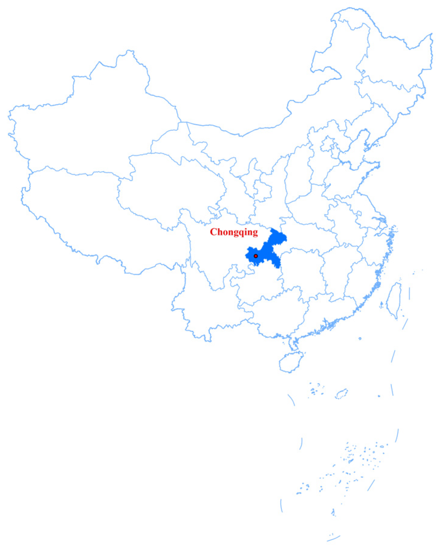
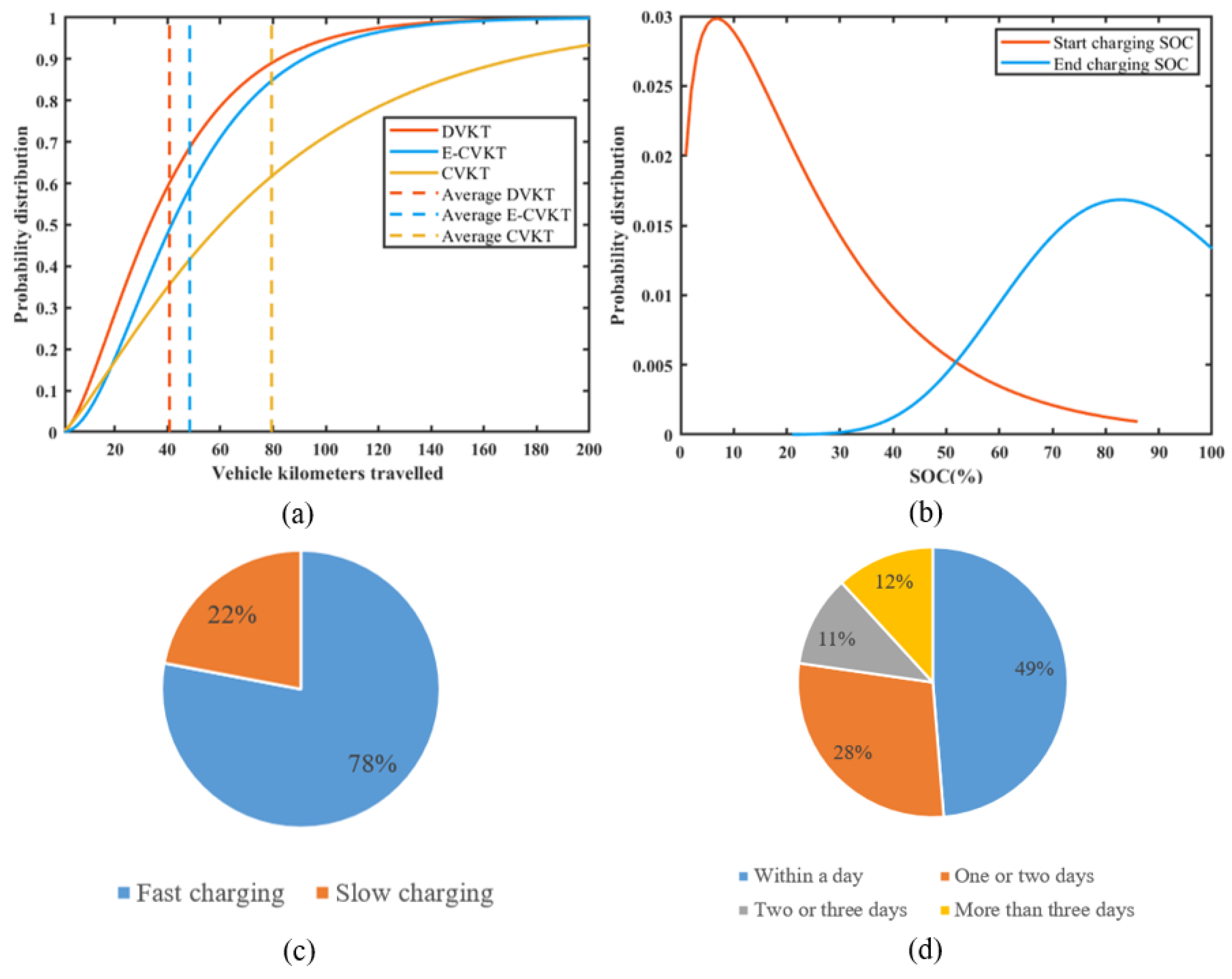
2.1. PHEV Data Description
- (1)
- Data cleaning
- (2)
- Trips segmentation
- (3)
- Outlier trip deletion
- (1)
- Discrete calculation of SOH
- (2)
- Fitting trends of SOH
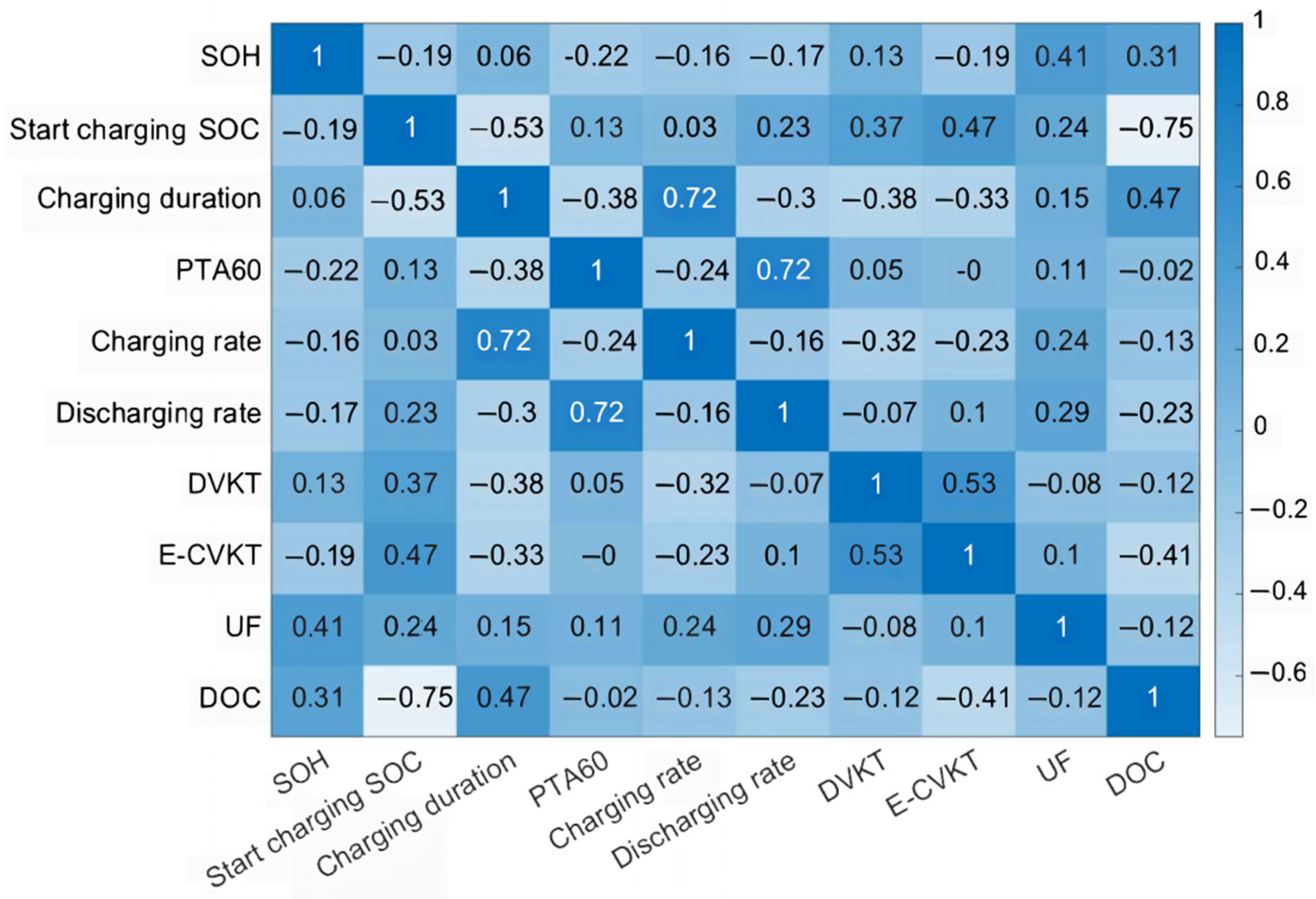
2.2. Correlation Analysis between Each Travel Feature
2.3. SOH Prediction of PHEVs
2.3.1. Degradation Calculation
- (1)
- SOH estimation
- (2)
- Degradation prediction
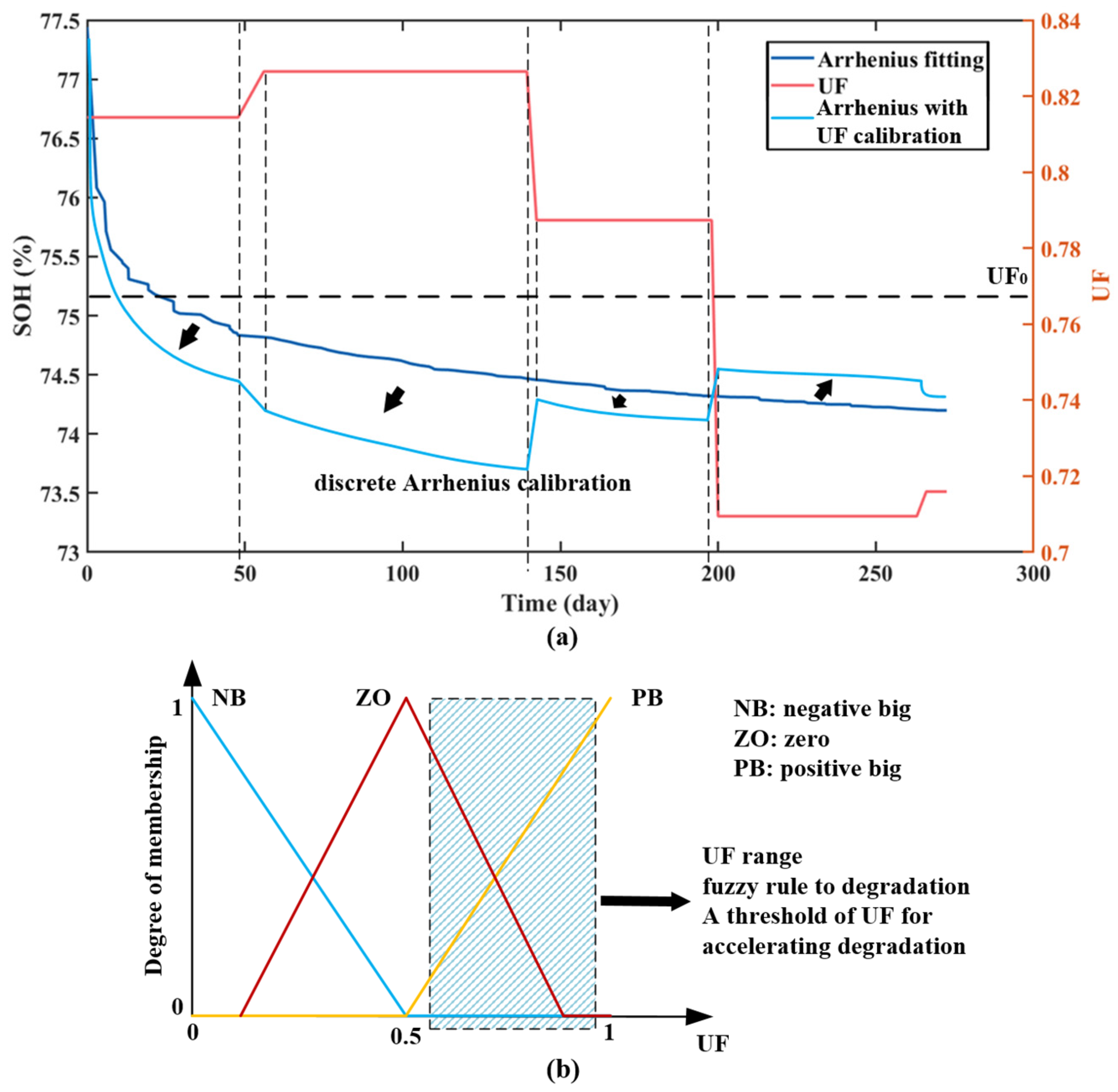
2.3.2. Degradation Calibration with PHEV Pattern
- (1)
- Discrete Arrhenius model
- (2)
- Calibration by UF
3. Experiment Results and Evaluation
3.1. Experiment Results
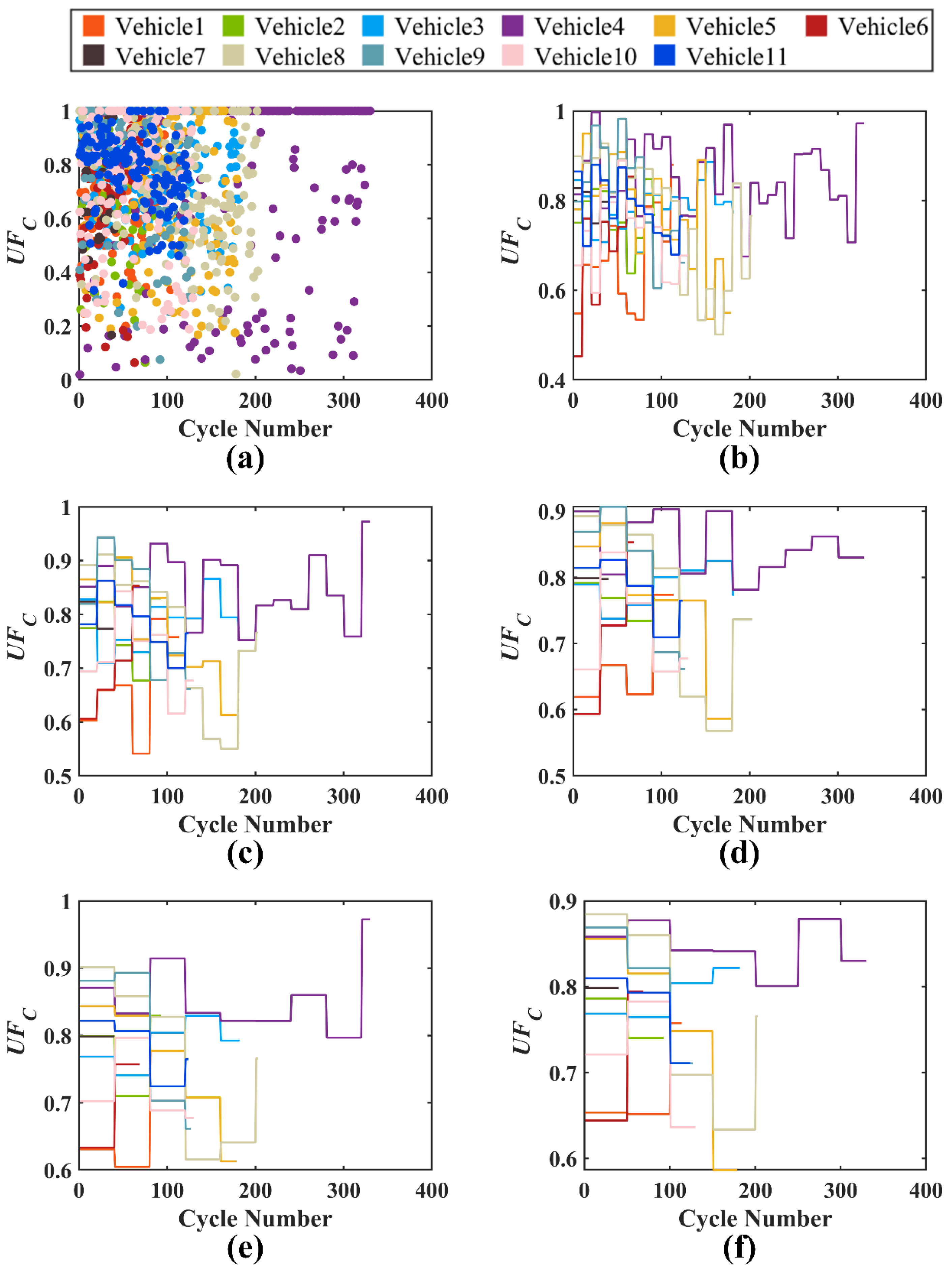
3.1.1. Optimal UF Selection
- (1)
- Step 1: the average values are calculated according to Equation (11) using different fixed cycle intervals (10, 20, 30, 40, and 50).
- (2)
- Step 2: the vehicle dataset is divided into two datasets as the calibration dataset and testing dataset. Based on the two datasets, the optimal threshold was determined using a certain optimal index that was calculated on the two datasets and the whole vehicle dataset.
- (3)
- Step 3: the calibration effects on the two datasets and the whole vehicle dataset were discussed. Then, the calibration effects of the optimal threshold in different fixed cycle intervals were also compared.
- (4)
- Step 4: the average values in different fixed cycle intervals were discussed to choose the optimal fixed cycle interval for practical calibration.
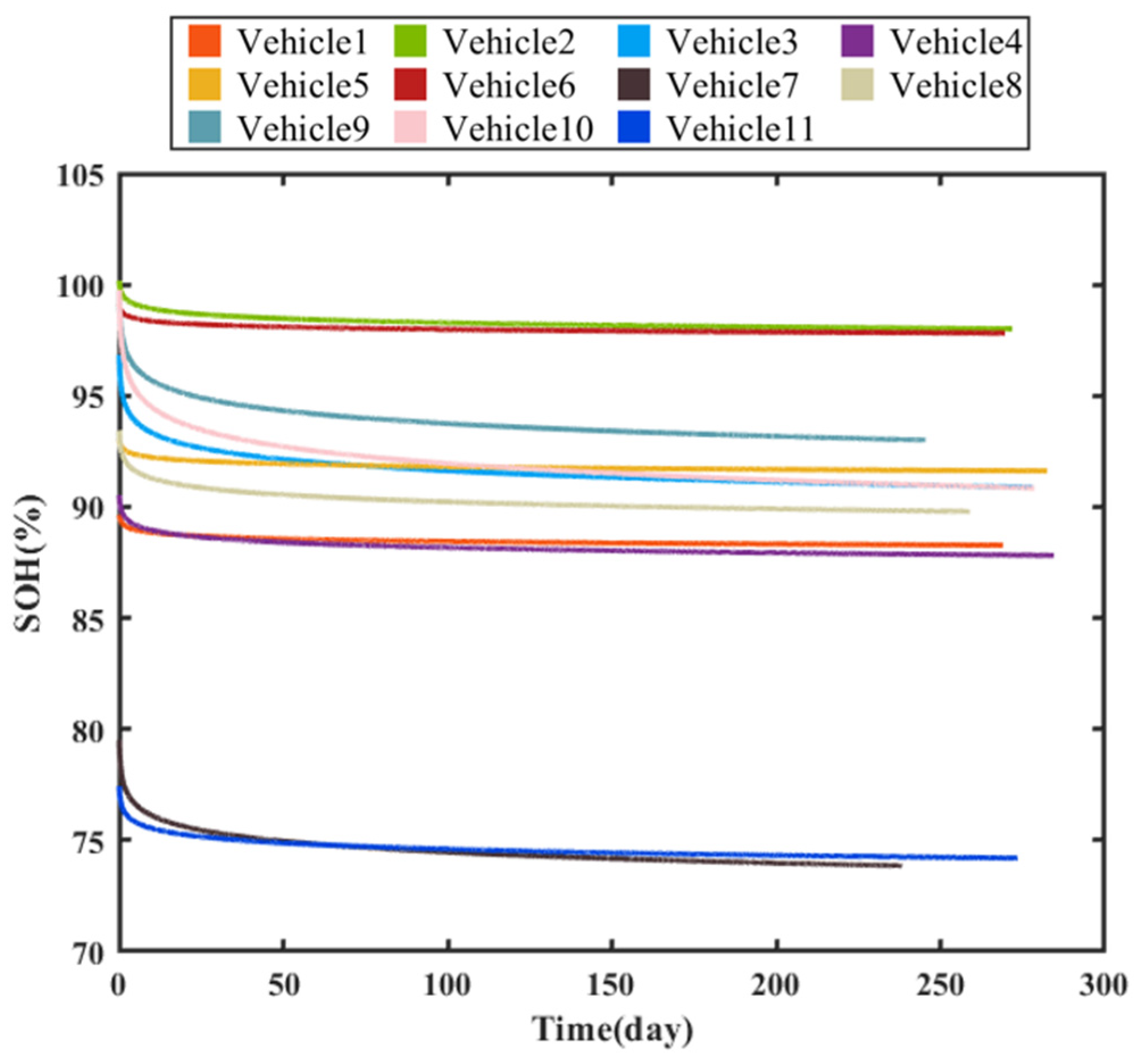
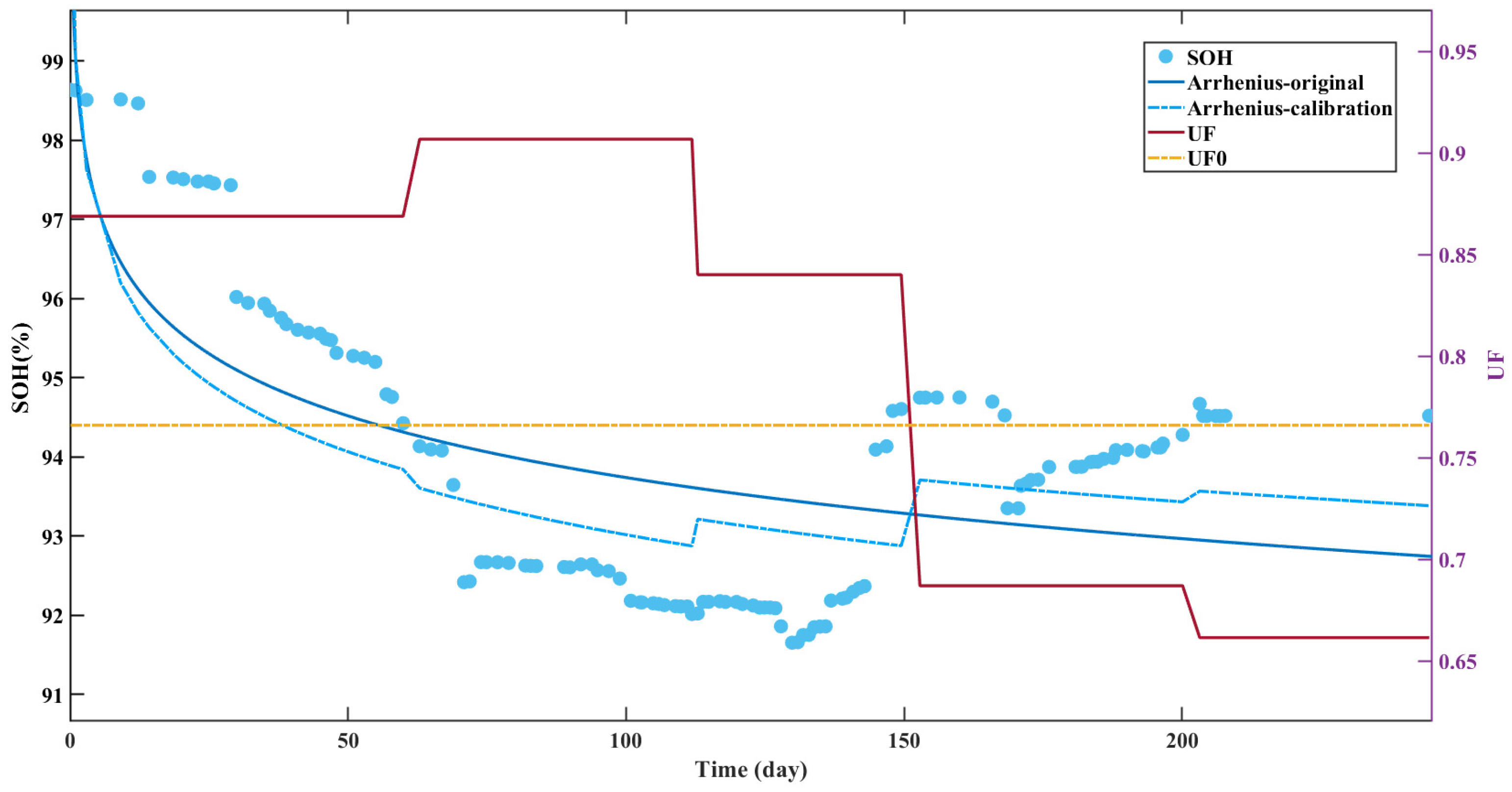
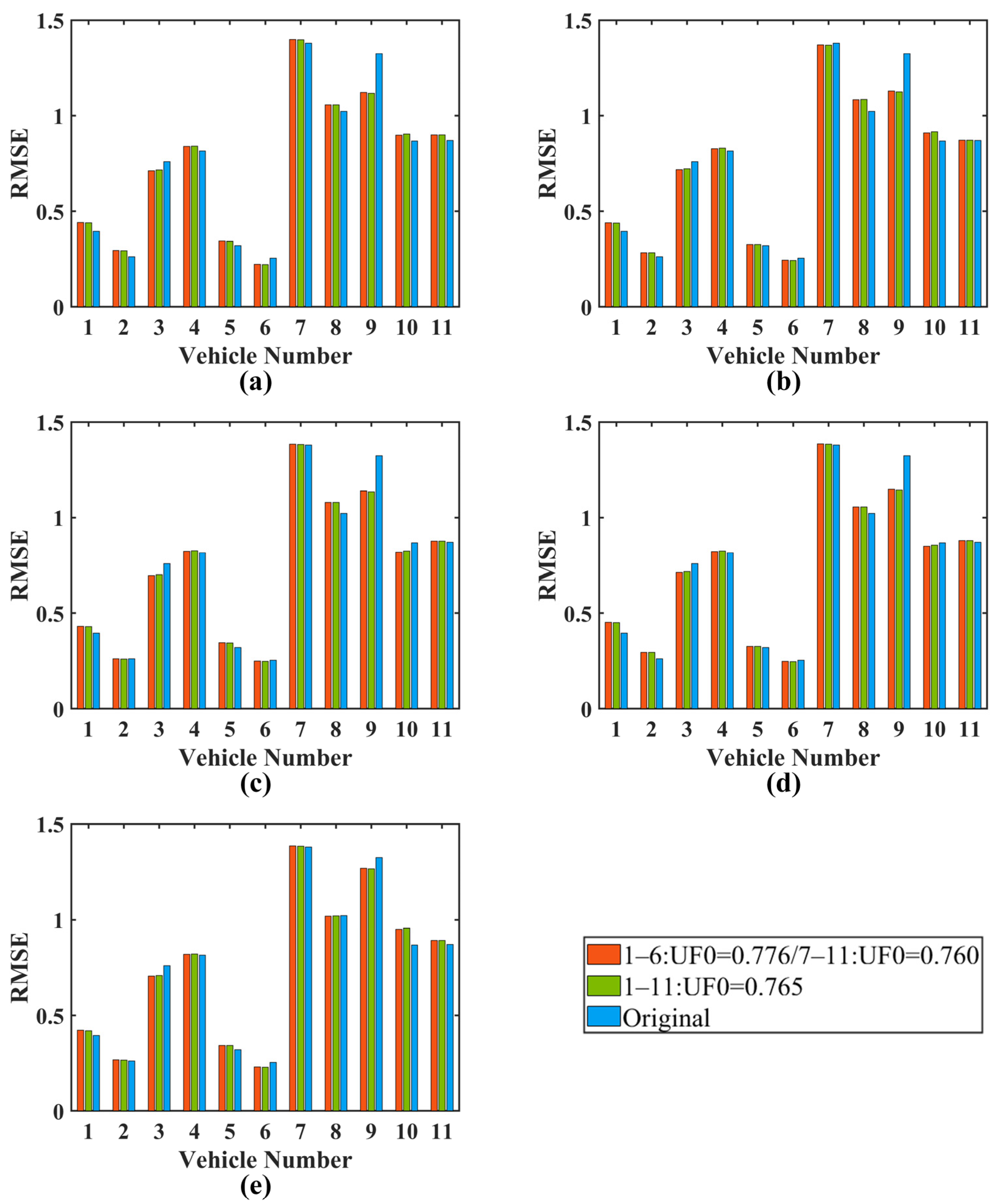
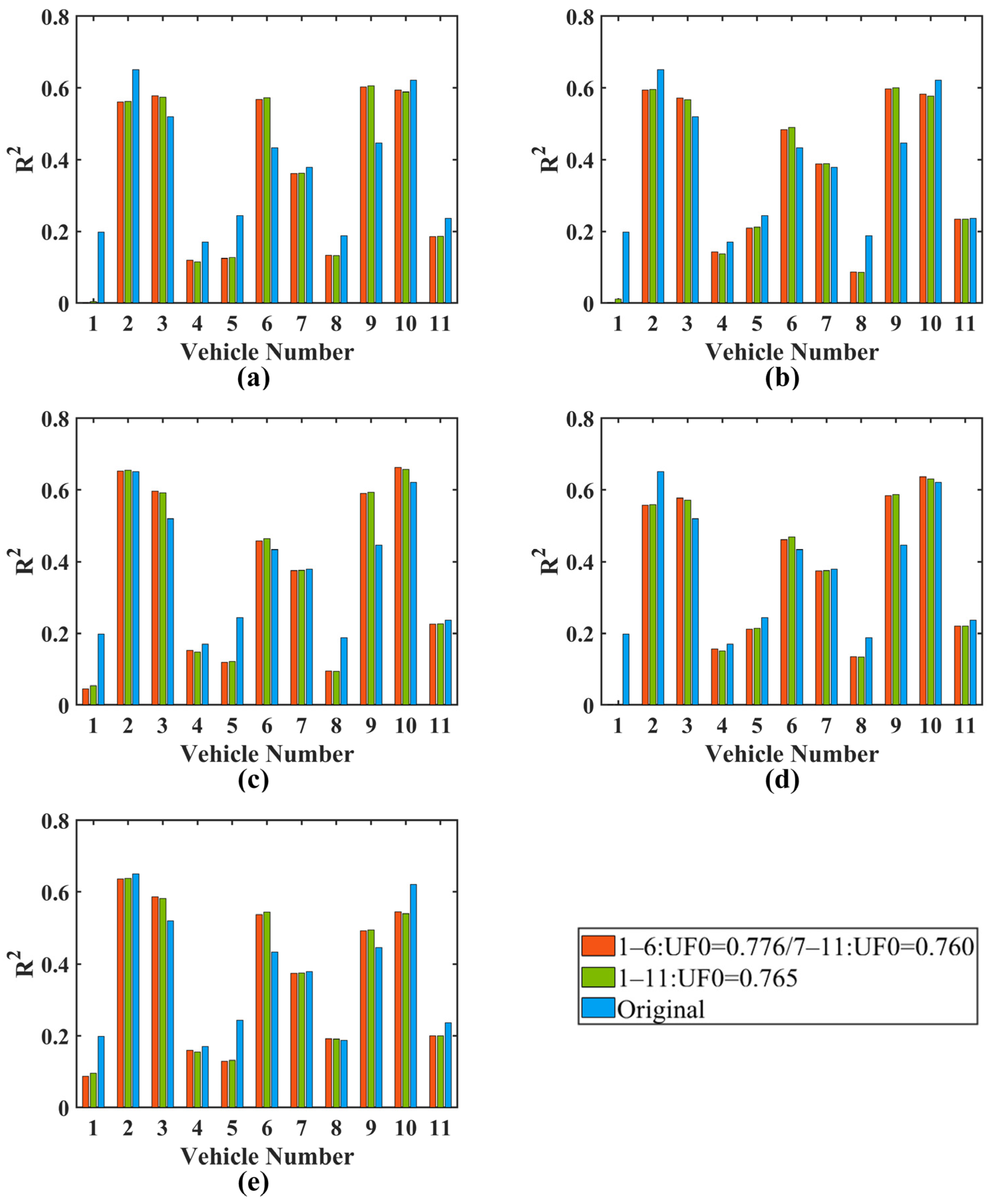
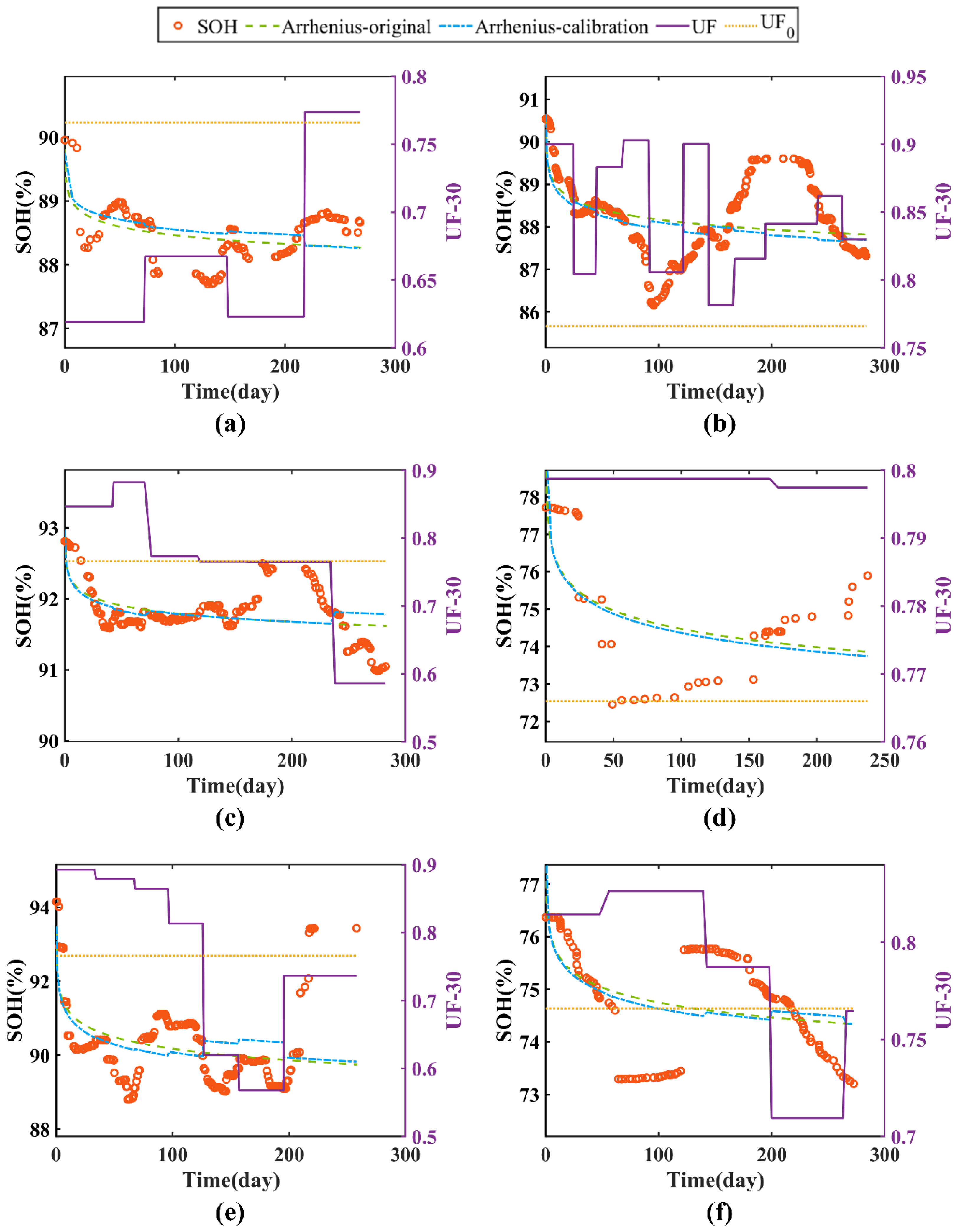
3.1.2. Calibration Results on Vehicle SOH Prediction
3.2. Calibration Effectiveness
3.3. Discussion
- (1)
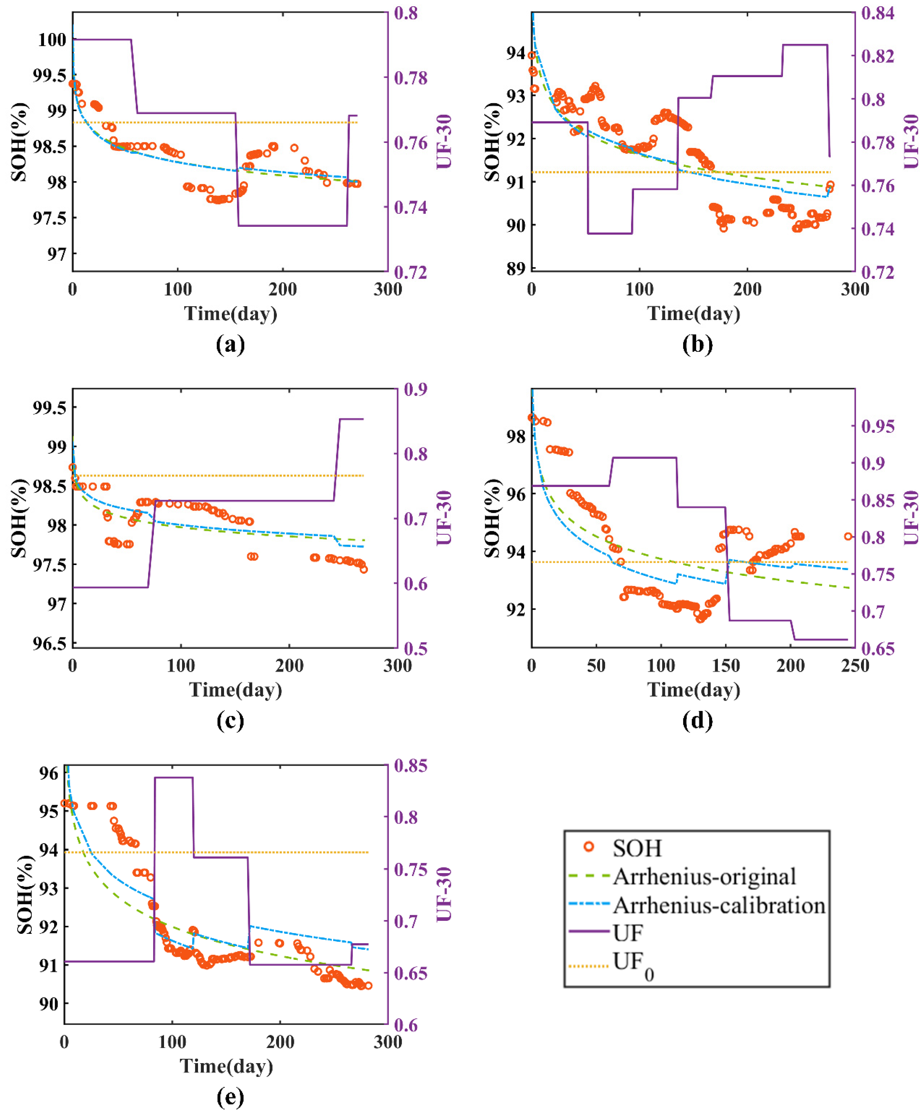
- For the 11 PHEVs in this work, the best UF calibration value was 0.776 and the best calibration cycle interval was 30. Using the best UF value and best cycle interval, the proposed calibration scheme can achieve an optimized calibration effects of SOH prediction for any set of PHEVs with a realistic dataset.
- (2)
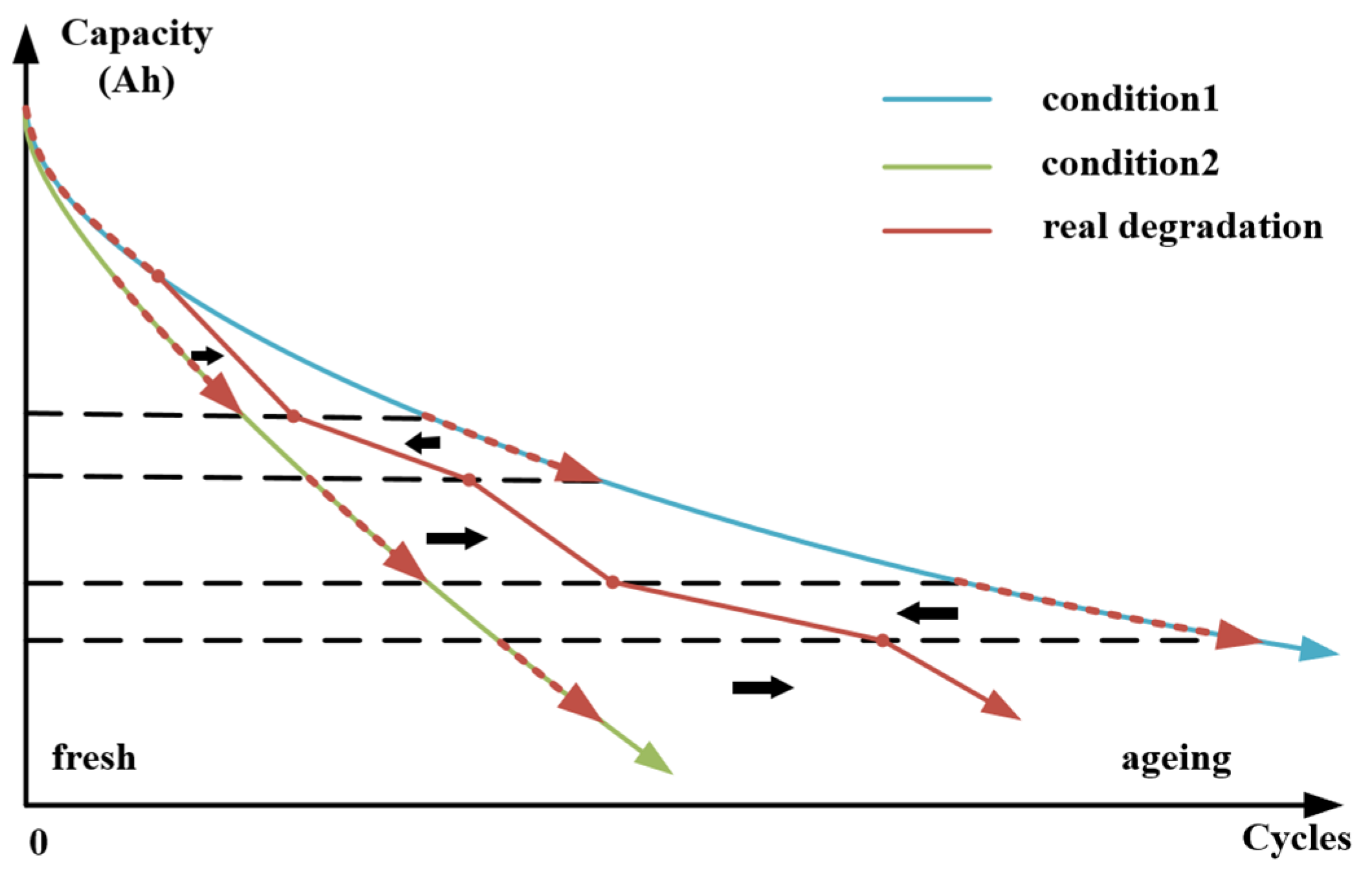
- The results show that a discrete Arrhenius curve is achieved after UF calibration, and the Arrhenius curve is no longer monotonous like a traditional battery degradation curve. We believe that the battery SOH should be discrete and fluctuant in every certain range after considering UF’s influence.
- (3)
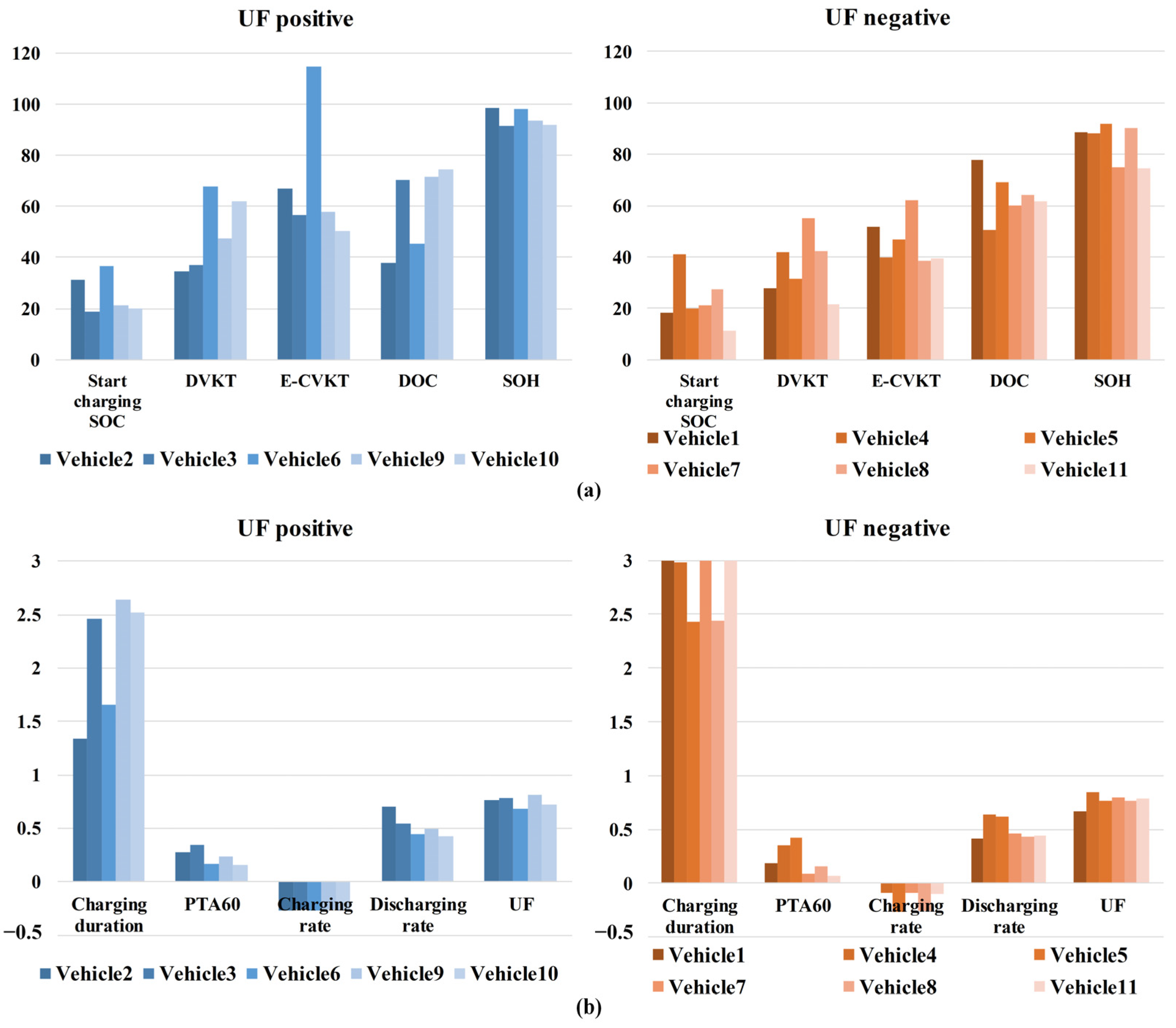
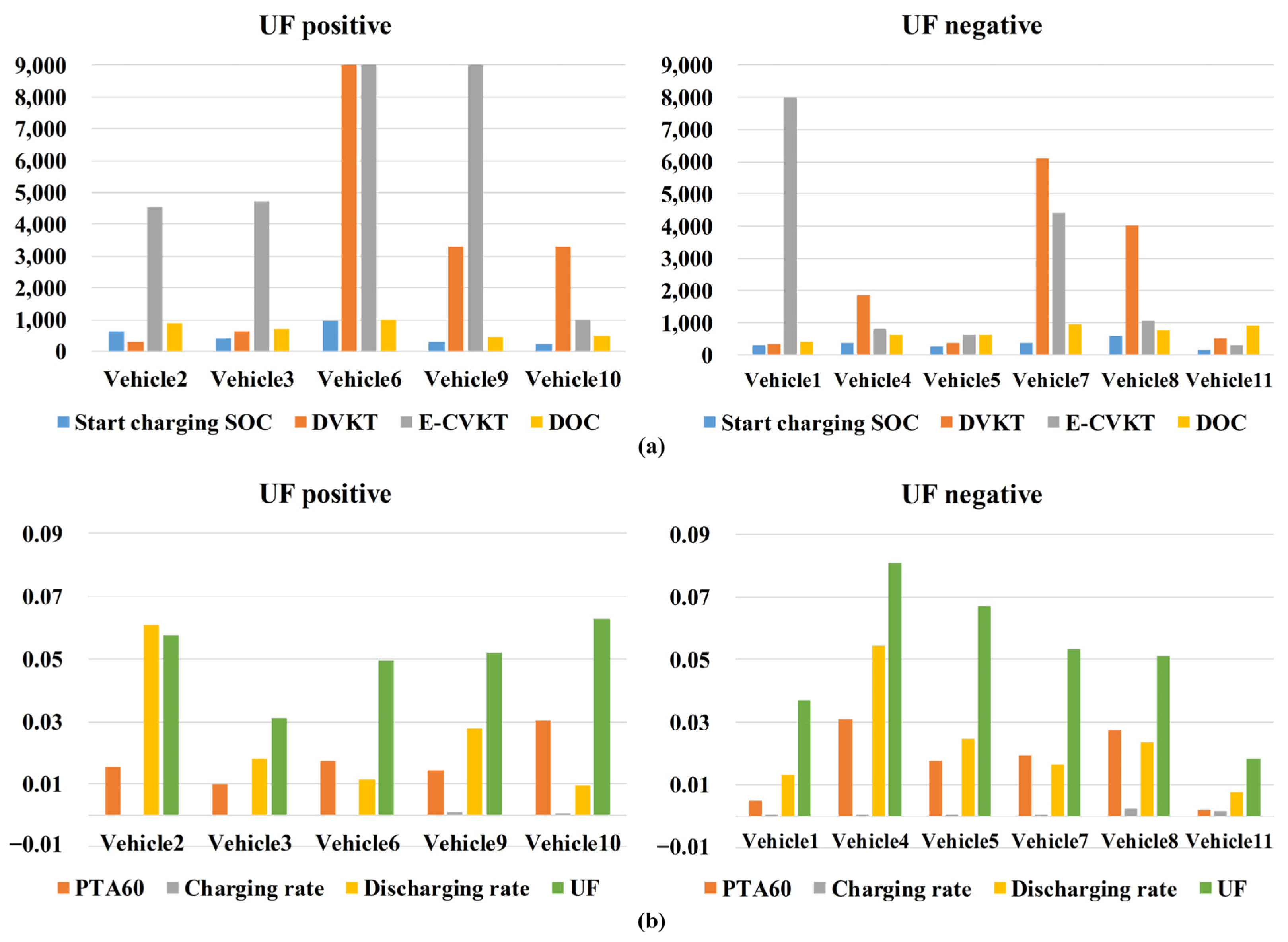
- According to Section 3.1.1, the UF threshold was optimized by using a pre-designed scheme that included the training vehicle dataset. It was found that the value of the UF threshold can be in a range to generate homogeneous calibration effects (positive or negative).
- (4)
- The proposed UF calibration method did have positive effects (smaller RMSE and larger R2) on some of the PHEVs. However, it showed negative effects for PHEVs with heavy degradation due to the inapplicability of Arrhenius fitting when the PHEV has large capacity loss.
4. Conclusions
Author Contributions
Funding
Data Availability Statement
Conflicts of Interest
Abbreviations
| BEV | Battery electric vehicle |
| DOC | Depth of charge |
| CVKT | Vehicle kilometers travelled during two charging sessions |
| DAAM | Discrete Arrhenius aging model |
| DVKT | Daily vehicle kilometers travelled |
| E-CVKT | Vehicle kilometers travelled during two charging sessions driven by electricity |
| CD | charging depleting |
| PEV | Plug-in electric vehicle |
| PHEV | Plug-in hybrid electric vehicle |
| PTA60 | Percentage of miles traveled above 60 km/h |
| RMSE | Root mean square error |
| SOC | State of charge |
| SOH | State of health |
| UF | Utility factor |
References
- International Energy Agency. Global EV Outlook 2022; IEA: Paris, France, 2022. [Google Scholar]
- Lopez-Ibarra, J.A.; Goitia-Zabaleta, N.; Isaac Herrera, V.; Gazta Naga, H.; Camblong, H. Battery aging conscious intelligent energy management strategy and sensitivity analysis of the critical factors for plug-in hybrid electric buses. eTransportation 2020, 5, 100061. [Google Scholar] [CrossRef]
- Ouyang, D.; Zhang, Q.; Ou, X. Review of Market Surveys on Consumer Behavior of Purchasing and Using Electric Vehicle in China. In Proceedings of the Applied Energy Symposium and Forum—Low-Carbon Cities and Urban Energy Systems (CUE), Shanghai, China, 5–7 June 2018; pp. 612–617. [Google Scholar]
- Hao, X.; Yuan, Y.; Wang, H.; Ouyang, M. Plug-in hybrid electric vehicle utility factor in China cities: Influencing factors, empirical research, and energy and environmental application. eTransportation 2021, 10, 100138. [Google Scholar] [CrossRef]
- Zubi, G.; Dufo-López, R.; Carvalho, M.; Pasaoglu, G. The lithium-ion battery: State of the art and future perspectives. Renew. Sustain. Energy Rev. 2018, 89, 292–308. [Google Scholar] [CrossRef]
- Wassiliadis, N.; Steinstraeter, M.; Schreiber, M.; Rosner, P.; Nicoletti, L.; Schmid, F.; Ank, M.; Teichert, O.; Wildfeuer, L.; Schneider, J.; et al. Quantifying the state of the art of electric powertrains in battery electric vehicles: Range, efficiency, and lifetime from component to system level of the Volkswagen ID.3. eTransportation 2022, 12, 100167. [Google Scholar] [CrossRef]
- Liu, K.; Liu, Y.Y.; Lin, D.C.; Pei, A.; Cui, Y. Materials for lithium-ion battery safety. Sci. Adv. 2018, 4, eaas9820. [Google Scholar] [CrossRef] [PubMed] [Green Version]
- Fotouhi, A.; Auger, D.J.; Propp, K.; Longo, S.; Wild, M. A review on electric vehicle battery modelling: From Lithium-ion toward Lithium-Sulphur. Renew. Sustain. Energy Rev. 2016, 56, 1008–1021. [Google Scholar] [CrossRef] [Green Version]
- Tian, H.X.; Qin, P.L.; Li, K.; Zhao, Z. A review of the state of health for lithium -ion batteries: Research status and suggestions. J. Clean. Prod. 2020, 261, 120813. [Google Scholar] [CrossRef]
- Berecibar, M.; Gandiaga, I.; Villarreal, I.; Omar, N.; Van Mierlo, J.; Van den Bossche, P. Critical review of state of health estimation methods of Li-ion batteries for real applications. Renew. Sustain. Energy Rev. 2016, 56, 572–587. [Google Scholar] [CrossRef]
- Zhang, J.; Lee, J. A review on prognostics and health monitoring of Li-ion battery. J. Power Sources 2011, 196, 6007–6014. [Google Scholar] [CrossRef]
- Zhang, H.; Qin, Y.; Li, X.; Liu, X.; Yan, J. Power management optimization in plug-in hybrid electric vehicles subject to uncertain driving cycles. eTransportation 2020, 3, 100029. [Google Scholar] [CrossRef]
- Li, X.; Yuan, C.; Wang, Z.; He, J.; Yu, S. Lithium battery state-of-health estimation and remaining useful lifetime prediction based on non-parametric aging model and particle filter algorithm. eTransportation 2022, 11, 100156. [Google Scholar] [CrossRef]
- Song, Z.; Yang, X.-G.; Yang, N.; Delgado, F.P.; Hofmann, H.; Sun, J. A study of cell-to-cell variation of capacity in parallel-connected lithium-ion battery cells. eTransportation 2021, 7, 100091. [Google Scholar] [CrossRef]
- Berecibar, M.; Garmendia, M.; Gandiaga, I.; Crego, J.; Villarreal, I. State of health estimation algorithm of LiFePO4 battery packs based on differential voltage curves for battery management system application. Energy 2016, 103, 784–796. [Google Scholar] [CrossRef]
- Goh, T.; Park, M.; Seo, M.; Kim, J.G.; Kim, S.W. Capacity estimation algorithm with a second-order differential voltage curve for Li-ion batteries with NMC cathodes. Energy 2017, 135, 257–268. [Google Scholar] [CrossRef]
- Li, X.; Wang, Z.; Zhang, L.; Zou, C.; Dorrell, D.D. State-of-health estimation for Li-ion batteries by combing the incremental capacity analysis method with grey relational analysis. J. Power Sources 2019, 410, 106–114. [Google Scholar] [CrossRef]
- Zheng, L.; Zhu, J.; Lu, D.D.-C.; Wang, G.; He, T. Incremental capacity analysis and differential voltage analysis based state of charge and capacity estimation for lithium-ion batteries. Energy 2018, 150, 759–769. [Google Scholar] [CrossRef]
- Jiang, B.; Dai, H.; Wei, X. Incremental capacity analysis based adaptive capacity estimation for lithium-ion battery considering charging condition. Appl. Energy 2020, 269, 115074. [Google Scholar] [CrossRef]
- Zhu, J.G.; Wang, Y.X.; Huang, Y.; Gopaluni, R.B.; Cao, Y.K.; Heere, M.; Muhlbauer, M.J.; Mereacre, L.; Dai, H.F.; Liu, X.H.; et al. Data-driven capacity estimation of commercial lithium-ion batteries from voltage relaxation. Nat. Commun. 2022, 13, 2261. [Google Scholar] [CrossRef]
- Qian, C.; Xu, B.; Chang, L.; Sun, B.; Feng, Q.; Yang, D.; Ren, Y.; Wang, Z. Convolutional neural network based capacity estimation using random segments of the charging curves for lithium-ion batteries. Energy 2021, 227, 120333. [Google Scholar] [CrossRef]
- Liu, J.Z.; Wang, Z.P.; Hou, Y.K.; Qu, C.H.; Hong, J.C.; Lin, N. Data-driven energy management and velocity prediction for four-wheel-independent-driving electric vehicles. eTransportation 2021, 9, 100119. [Google Scholar] [CrossRef]
- Su, L.; Wu, M.; Li, Z.; Zhang, J. Cycle life prediction of lithium-ion batteries based on data-driven methods. eTransportation 2021, 10, 100137. [Google Scholar] [CrossRef]
- Waag, W.; Fleischer, C.; Sauer, D.U. Critical review of the methods for monitoring of lithium-ion batteries in electric and hybrid vehicles. J. Power Sources 2014, 258, 321–339. [Google Scholar] [CrossRef]
- Zheng, Y.; Qin, C.; Lai, X.; Han, X.; Xie, Y. A novel capacity estimation method for lithium-ion batteries using fusion estimation of charging curve sections and discrete Arrhenius aging model. Appl. Energy 2019, 251, 113327. [Google Scholar] [CrossRef]
- Li, K.; Zhou, P.; Lu, Y.; Han, X.; Li, X.; Zheng, Y. Battery life estimation based on cloud data for electric vehicles. J. Power Sources 2020, 468, 228192. [Google Scholar] [CrossRef]
- Khalid, A.; Sarwat, A.I. Fast Charging Li-Ion Battery Capacity Fade Prognostic Modeling Using Correlated Parameters’ Decomposition and Recurrent Wavelet Neural Network. In Proceedings of the IEEE Transportation Electrification Conference and Expo (ITEC), Electr Network, Chicago, IL, USA, 21–25 June 2021; pp. 27–32. [Google Scholar]
- Davies, J.; Kurani, K.S. Moving from assumption to observation: Implications for energy and emissions impacts of plug-in hybrid electric vehicles. Energy Policy 2013, 62, 550–560. [Google Scholar] [CrossRef]
- Duhon, A.N.; Sevel, K.S.; Tarnowsky, S.A.; Savagian, P.J. Chevrolet volt electric utilization. SAE Int. J. Altern. Powertrains 2015, 4, 269–276. [Google Scholar] [CrossRef]
- Kelly, J.C.; MacDonald, J.S.; Keoleian, G.A. Time-dependent plug-in hybrid electric vehicle charging based on national driving patterns and demographics. Appl. Energy 2012, 94, 395–405. [Google Scholar] [CrossRef]
- Goebel, D.; Plotz, P. Machine learning estimates of plug-in hybrid electric vehicle utility factors. Transp. Res. Part D-Transp. Environ. 2019, 72, 36–46. [Google Scholar] [CrossRef]
- GB/T 32960.3-2016; Technical Specifications of Eemote Service and Management System for Electric Vehicles–Part 3: Communication Protocol and Data Format. National Standard of the People’s Republic of China: Beijing, China, 2016.
- Duoba, M. Developing a utility factor for battery electric vehicles. SAE Int. J. Altern. Powertrains 2013, 2, 362–368. [Google Scholar] [CrossRef]
- Zheng, Y.J.; Cui, Y.F.; Han, X.B.; Ouyang, M.G. A capacity prediction framework for lithium-ion batteries using fusion prediction of empirical model and data-driven method. Energy 2021, 237, 121556. [Google Scholar] [CrossRef]
- Han, X. Study on Li-ion Battery Mechanism Model and State Estimation for Electric Vehicles. Ph.D. Thesis, Tsinghua University, Beijing, China, 2014. [Google Scholar]


| Data | Meaning and Provisions |
|---|---|
| Battery charge status | 1—Parking charge; 2—Driving charge; 3—Uncharged |
| Total odometer | Vehicle’s total mileage (km) |
| Speed | Speed of a vehicle (km/h) |
| SOC | State of charge |
| Terminal time | Running time |
| Vehicle operation state | The type of power used to propel the vehicle during operation: 1—Pure electric; 2—Hybrid electric; 3—Oil fuel |
| Total voltage | Battery voltage (V) |
| Total current | Battery current (A) |
| Data | Description |
|---|---|
| Number of vehicles | 11 |
| Total mileage | 13,590 km |
| Average driving days | 233 |
| Average DVKT | 41 km |
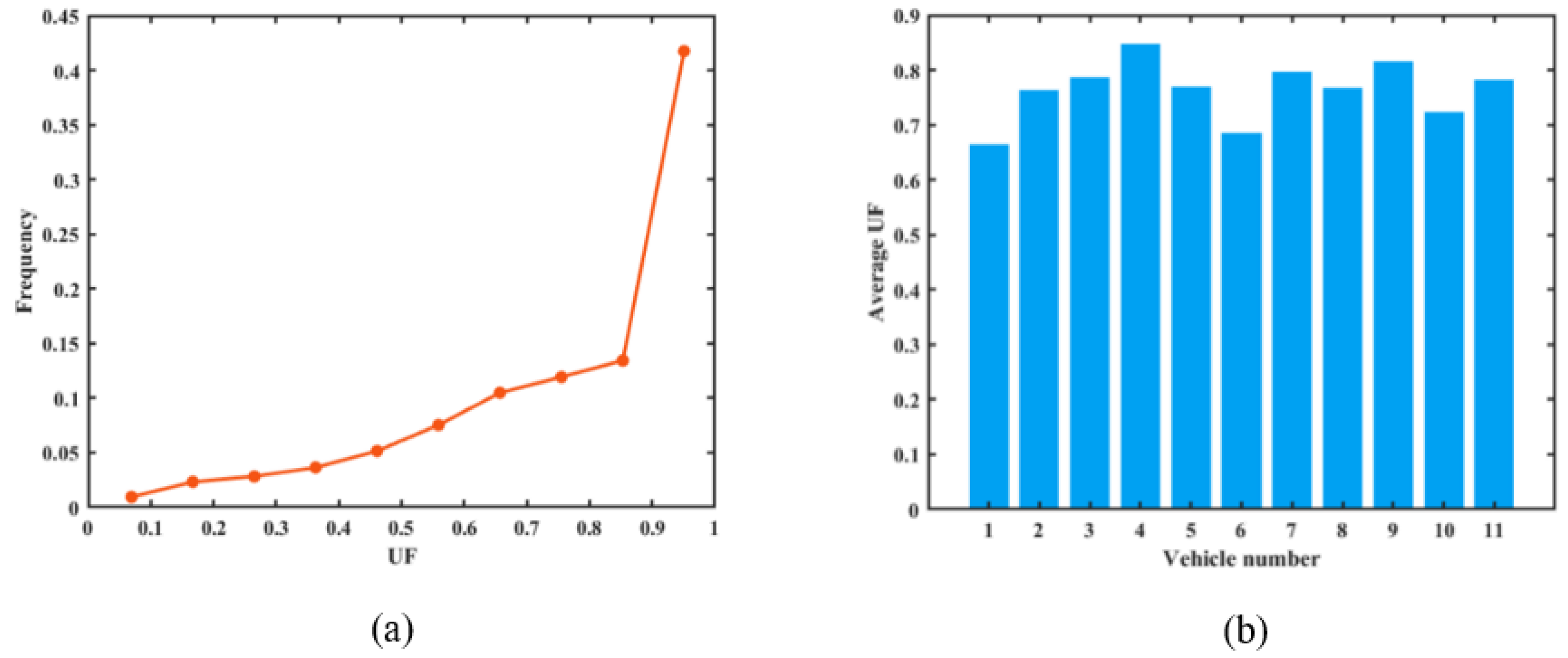
| Average utility factor | 0.87 |
| Average start charging SOC | 22% |
| Average end charging SOC | 86% |
| Percentage of miles traveled above 60 km/h | 22% |
| Start Charging SOC | Charging Duration (h) | PTA60 | Charging Rate | Discharging Rate | DVKT (km) | E-CVKT (km) | UF | DOC | |
|---|---|---|---|---|---|---|---|---|---|
| Correlation coefficients | −0.19 | 0.06 | −0.22 | −0.16 | −0.17 | 0.13 | −0.19 | 0.41 | 0.31 |
| 10 | 20 | 30 | 40 | 50 | ||
|---|---|---|---|---|---|---|
| Sets | ||||||
| Entire set | 0.765 | 0.764 | 0.764 | 0.764 | 0.764 | |
| Calibration set | 0.776 | 0.775 | 0.775 | 0.776 | 0.774 | |
| Test set | 0.760 | 0.759 | 0.759 | 0.759 | 0.760 | |
| 10 | 20 | 30 | 40 | 50 | ||
|---|---|---|---|---|---|---|
| Effects | ||||||
| Vehicle with positive calibration | 3, 6, 9 | 3, 6, 7, 9 | 2, 3, 6, 9, 10 | 3, 6, 9, 10 | 3, 6, 8, 9 | |
| Vehicle with negative calibration | 1, 2, 4, 5, 7, 8, 10, 11 | 1, 2, 4, 5, 8, 10, 11 | 1, 4, 5, 7, 8, 11 | 1, 2, 4, 5, 7, 8, 11 | 1, 2, 4, 5, 7, 10, 11 | |
| Amount of positive calibration | 3 | 4 | 5 | 4 | 4 | |
| Vehicle Number | Start Charging SOC | Charging Duration | PTA60 | Charging Rate | Discharging Rate | DVKT | E-CVKT | DOC | SOH | UF |
|---|---|---|---|---|---|---|---|---|---|---|
| Vehicle1 | 18.3333 | 3.0907 | 0.1830 | −90.2240 | 0.4113 | 27.6833 | 51.6140 | 77.7544 | 88.4334 | 0.6654 |
| Vehicle2 * | 31.2151 | 1.3422 | 0.2745 | −0.2714 | 0.7077 | 34.4961 | 66.9247 | 37.9677 | 98.3576 | 0.7650 |
| Vehicle3 * | 18.8022 | 2.4672 | 0.3492 | −0.2641 | 0.5434 | 36.8714 | 56.4286 | 70.3132 | 91.6116 | 0.7867 |
| Vehicle4 | 41.0091 | 2.9802 | 0.3585 | −0.0864 | 0.6386 | 41.8517 | 39.7039 | 50.6707 | 88.1795 | 0.8484 |
| Vehicle5 | 19.8045 | 2.4352 | 0.4264 | −0.2628 | 0.6197 | 31.3655 | 46.7263 | 68.9050 | 91.8248 | 0.7708 |
| Vehicle6 * | 36.4857 | 1.6542 | 0.1682 | −0.2689 | 0.4479 | 67.7194 | 114.5714 | 45.3143 | 98.0118 | 0.6869 |
| Vehicle7 | 21.3000 | 5.6298 | 0.0865 | −0.0880 | 0.4593 | 55.1220 | 61.9500 | 60.0500 | 74.8514 | 0.7984 |
| Vehicle8 | 27.3054 | 2.4416 | 0.1552 | −0.2517 | 0.4370 | 42.4369 | 38.4483 | 64.2365 | 90.3339 | 0.7688 |
| Vehicle9 * | 21.3386 | 2.6462 | 0.2336 | −0.2641 | 0.4946 | 47.3295 | 57.7402 | 71.7087 | 93.7153 | 0.8166 |
| Vehicle10 * | 19.8154 | 2.5214 | 0.1560 | −0.2683 | 0.4252 | 61.9287 | 50.3846 | 74.2308 | 91.9104 | 0.7253 |
| Vehicle11 | 11.0403 | 5.4652 | 0.0707 | −0.1027 | 0.4461 | 21.6249 | 39.2500 | 61.6774 | 74.6177 | 0.7838 |
| Vehicle Number | Start Charging SOC | Charging Duration | PTA60 | Charging Rate | Discharging Rate | DVKT | E-CVKT | DOC | SOH | UF |
|---|---|---|---|---|---|---|---|---|---|---|
| Vehicle1 | 313.9764 | 0.5984 | 0.0048 | 0.0001 | 0.0131 | 334.8532 | 7975.6550 | 401.8683 | 0.0308 | 0.0371 |
| Vehicle2 * | 636.7576 | 1.0926 | 0.0156 | 0.0000 | 0.0610 | 315.9398 | 4548.3747 | 906.4881 | 0.1291 | 0.0575 |
| Vehicle3 * | 425.1098 | 0.8166 | 0.0100 | 0.0001 | 0.0182 | 652.7748 | 4736.5114 | 709.0561 | 0.6200 | 0.0310 |
| Vehicle4 | 392.5302 | 2.6077 | 0.0310 | 0.0000 | 0.0544 | 1871.7027 | 826.2454 | 620.2640 | 0.1366 | 0.0810 |
| Vehicle5 | 270.3941 | 0.7513 | 0.0174 | 0.0001 | 0.0248 | 365.9159 | 617.7168 | 630.7943 | 0.0401 | 0.0670 |
| Vehicle6 * | 966.6302 | 1.2820 | 0.0173 | 0.0002 | 0.0112 | 9389.7177 | 18,610.7702 | 994.2766 | 0.0408 | 0.0496 |
| Vehicle7 | 363.4462 | 7.5441 | 0.0194 | 0.0002 | 0.0164 | 6124.3277 | 4429.4846 | 945.7410 | 1.1835 | 0.0532 |
| Vehicle8 | 611.4607 | 1.6979 | 0.0271 | 0.0024 | 0.0237 | 4011.1059 | 1080.0010 | 767.7854 | 0.2517 | 0.0510 |
| Vehicle9 * | 307.5273 | 1.2750 | 0.0143 | 0.0011 | 0.0279 | 3289.4916 | 16,368.9240 | 451.8906 | 0.6160 | 0.0522 |
| Vehicle10 * | 242.1827 | 0.4657 | 0.0303 | 0.0005 | 0.0096 | 3302.4934 | 988.7346 | 496.4890 | 1.3840 | 0.0629 |
| Vehicle11 | 152.7219 | 7.7078 | 0.0021 | 0.0016 | 0.0075 | 539.0179 | 306.5630 | 907.7488 | 0.2238 | 0.0185 |
Disclaimer/Publisher’s Note: The statements, opinions and data contained in all publications are solely those of the individual author(s) and contributor(s) and not of MDPI and/or the editor(s). MDPI and/or the editor(s) disclaim responsibility for any injury to people or property resulting from any ideas, methods, instructions or products referred to in the content. |
© 2023 by the authors. Licensee MDPI, Basel, Switzerland. This article is an open access article distributed under the terms and conditions of the Creative Commons Attribution (CC BY) license (https://creativecommons.org/licenses/by/4.0/).
Share and Cite
Cai, H.; Hao, X.; Jiang, Y.; Wang, Y.; Han, X.; Yuan, Y.; Zheng, Y.; Wang, H.; Ouyang, M. Degradation Evaluation of Lithium-Ion Batteries in Plug-In Hybrid Electric Vehicles: An Empirical Calibration. Batteries 2023, 9, 321. https://doi.org/10.3390/batteries9060321
Cai H, Hao X, Jiang Y, Wang Y, Han X, Yuan Y, Zheng Y, Wang H, Ouyang M. Degradation Evaluation of Lithium-Ion Batteries in Plug-In Hybrid Electric Vehicles: An Empirical Calibration. Batteries. 2023; 9(6):321. https://doi.org/10.3390/batteries9060321
Chicago/Turabian StyleCai, Hongchang, Xu Hao, Yong Jiang, Yanan Wang, Xuebing Han, Yuebo Yuan, Yuejiu Zheng, Hewu Wang, and Minggao Ouyang. 2023. "Degradation Evaluation of Lithium-Ion Batteries in Plug-In Hybrid Electric Vehicles: An Empirical Calibration" Batteries 9, no. 6: 321. https://doi.org/10.3390/batteries9060321