
Influence of Lithium-Ion-Battery Equivalent Circuit Model Parameter Dependencies and Architectures on the Predicted Heat Generation in Real-Life Drive Cycles


Abstract
:1. Introduction
2. Methodology
2.1. Electric Equivalent Circuit Models for Lithium-Ion-Batteries
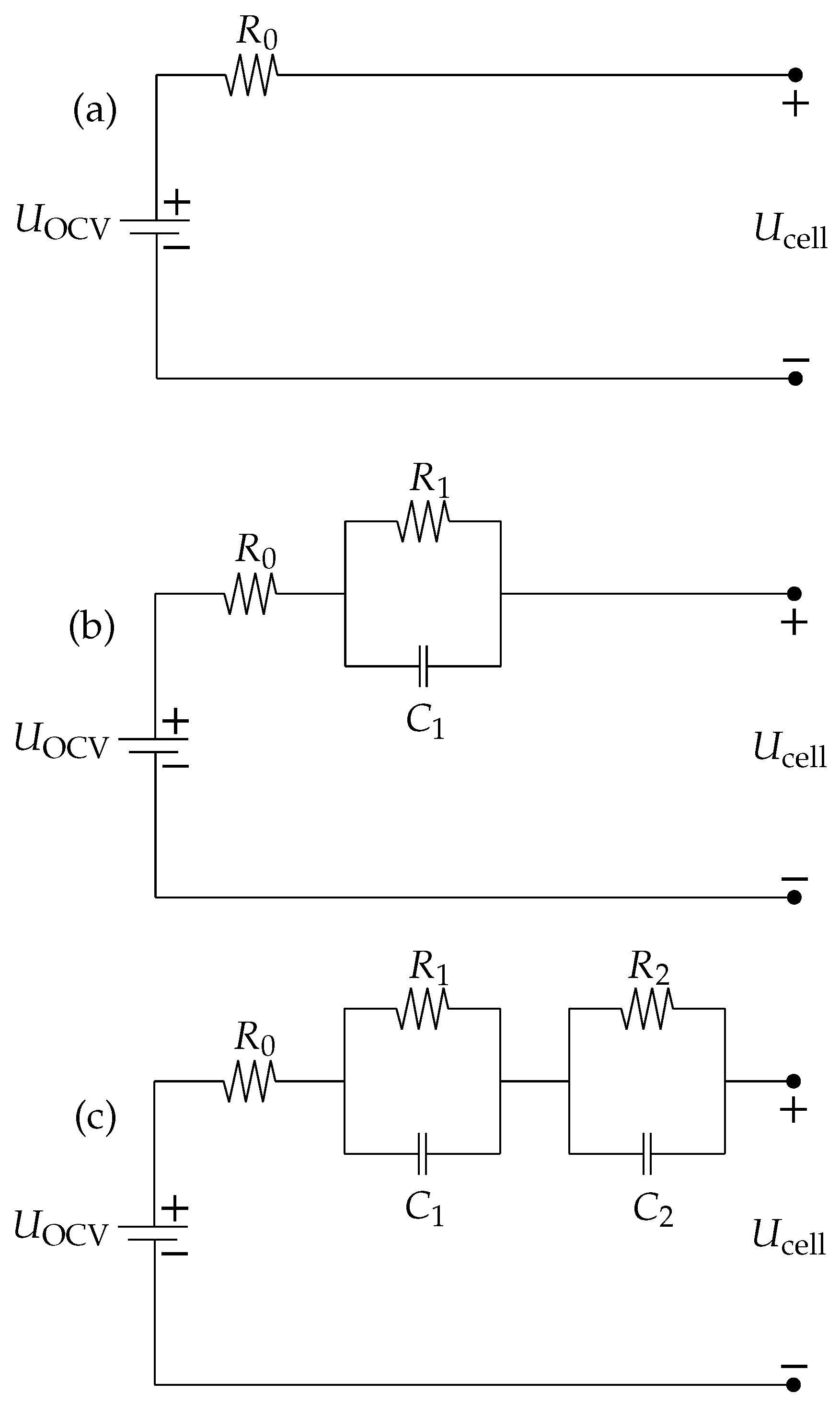
2.1.1. The Rint Model
2.1.2. The Thevenin Model
2.1.3. The Dual Polarization Model
2.1.4. Dependencies
2.1.5. State of Charge Estimation
2.2. Heat Generation Calculation
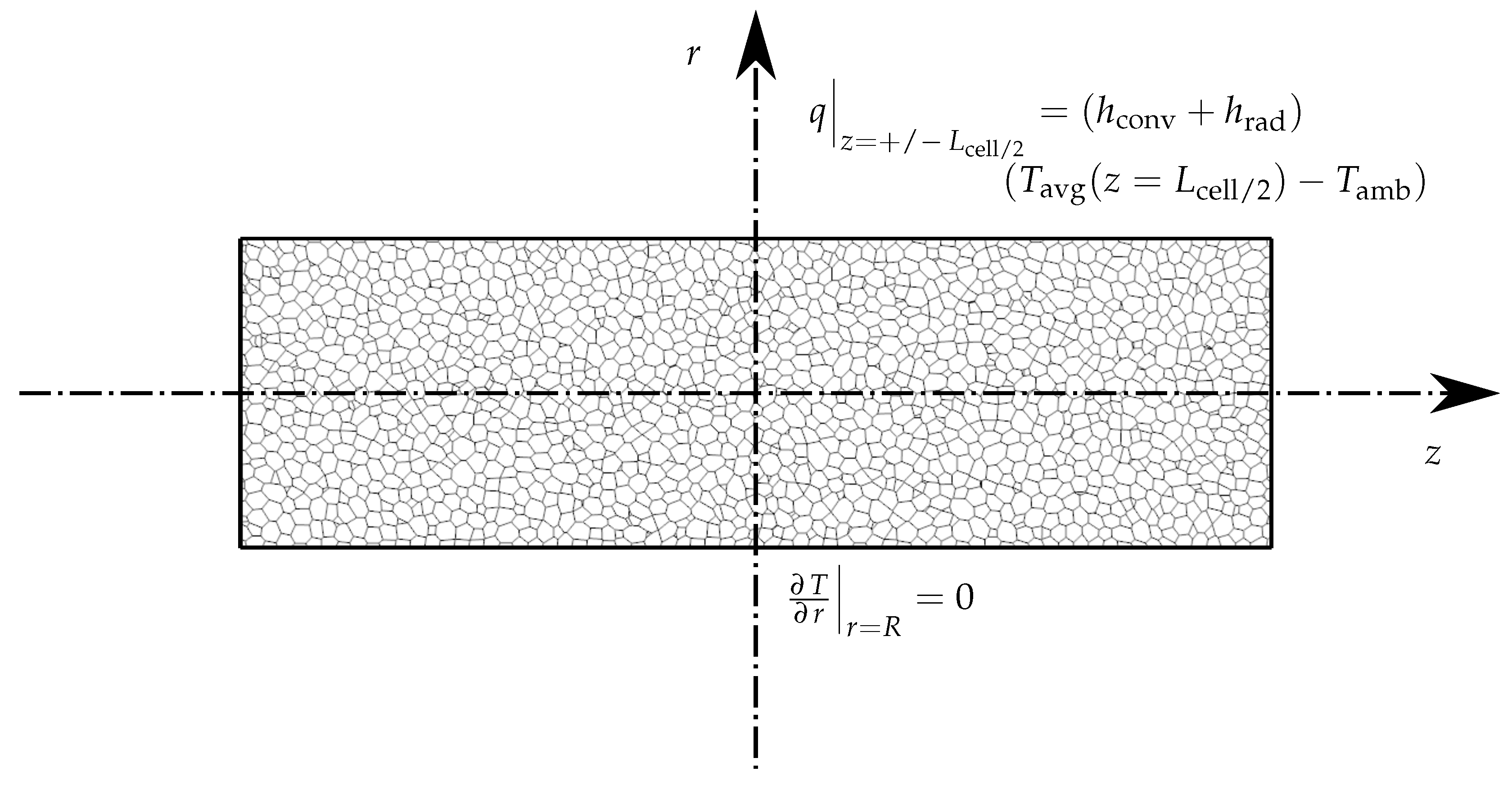
2.3. Thermal Model
2.3.1. Assumptions
2.3.2. Heat Convection and Heat Radiation
3. Experimental Setup and Parameter Identification
3.1. Battery Test Bench
3.1.1. Capacity Test
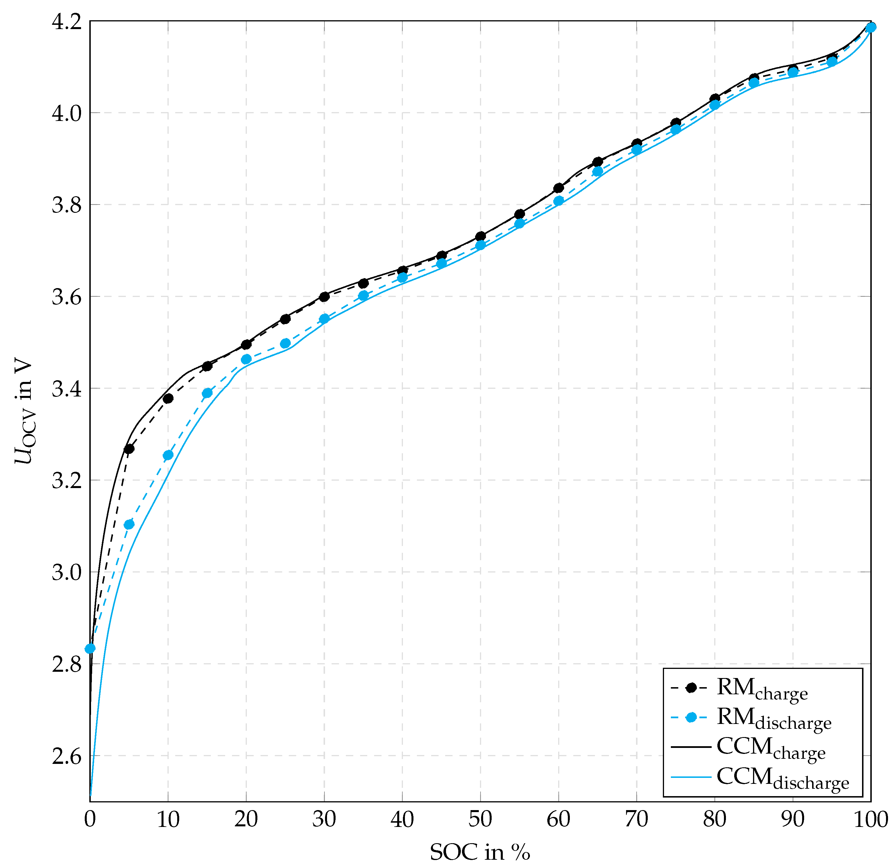
3.1.2. OCV-SOC Test
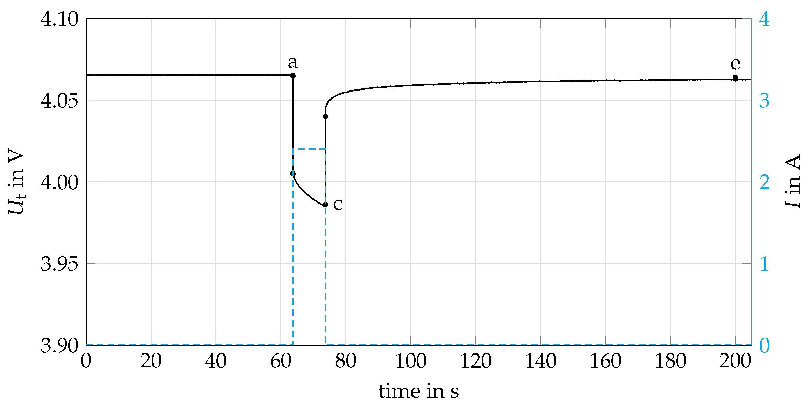
3.1.3. HPPC Test
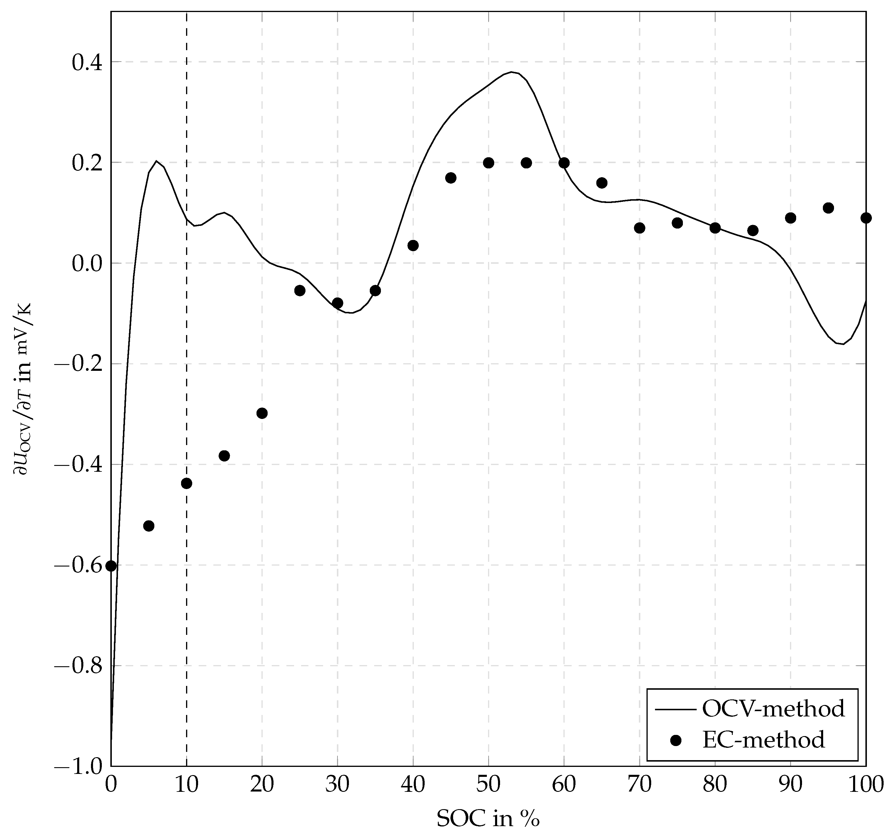
3.1.4. Entropic Coefficient Test
3.2. ECM Parameter Identification
3.2.1. Open Circuit Voltage
3.2.2. Resistances and Capacitances
4. Results and Discussion
4.1. Experimental Results
4.1.1. Capacity Test Results
4.1.2. OCV-SOC Test Results
4.1.3. HPPC Test Results
4.1.4. Entropic Coefficient Test Results
4.2. Thermal Modeling Results
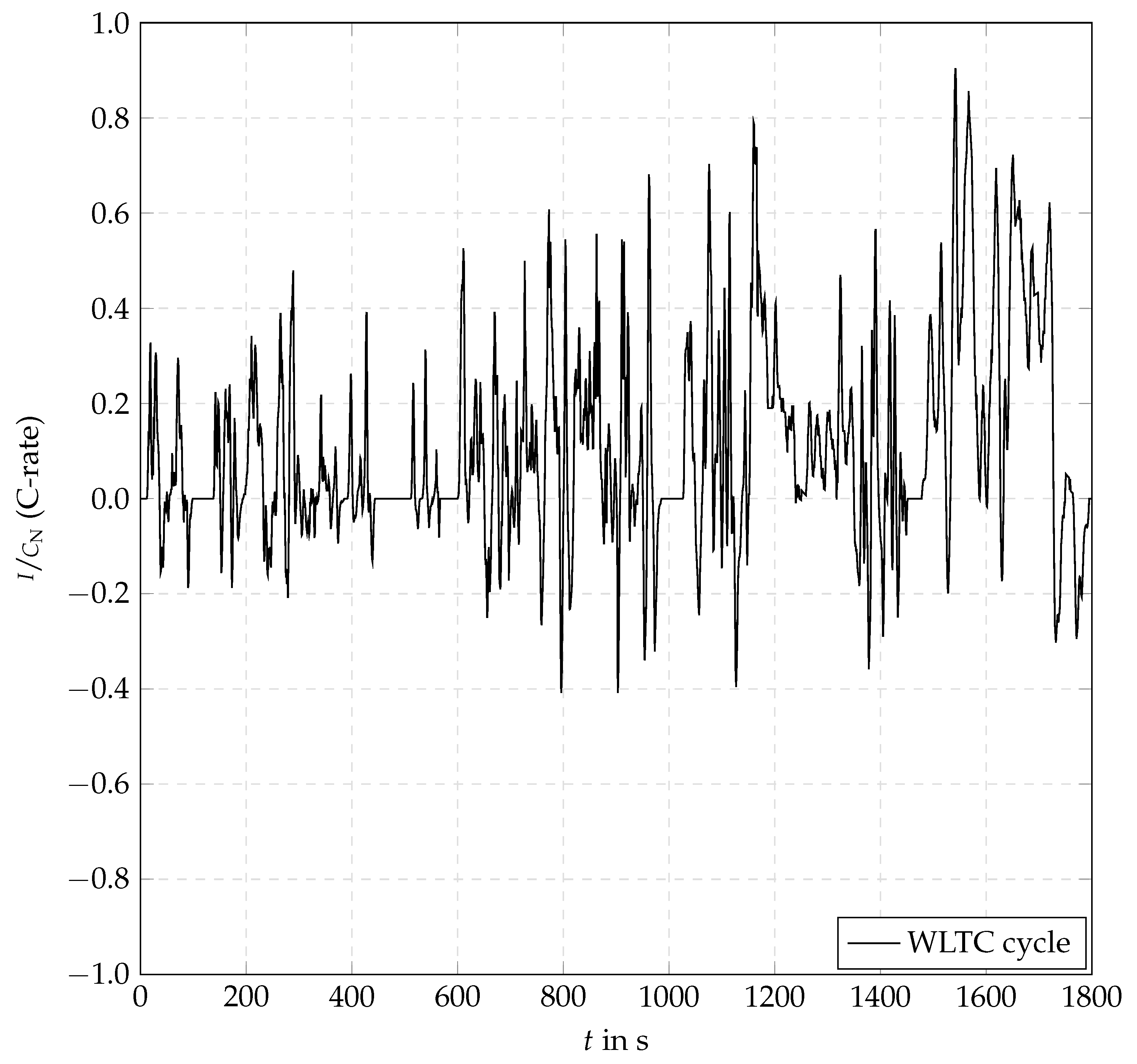
4.3. Validation Profile
4.4. Voltage Validation and Comparison ECMs
4.4.1. Assumptions
4.4.2. ECM Parameter Dependencies
4.4.3. ECM Test Parameter
4.4.4. ECM Architecture Influence
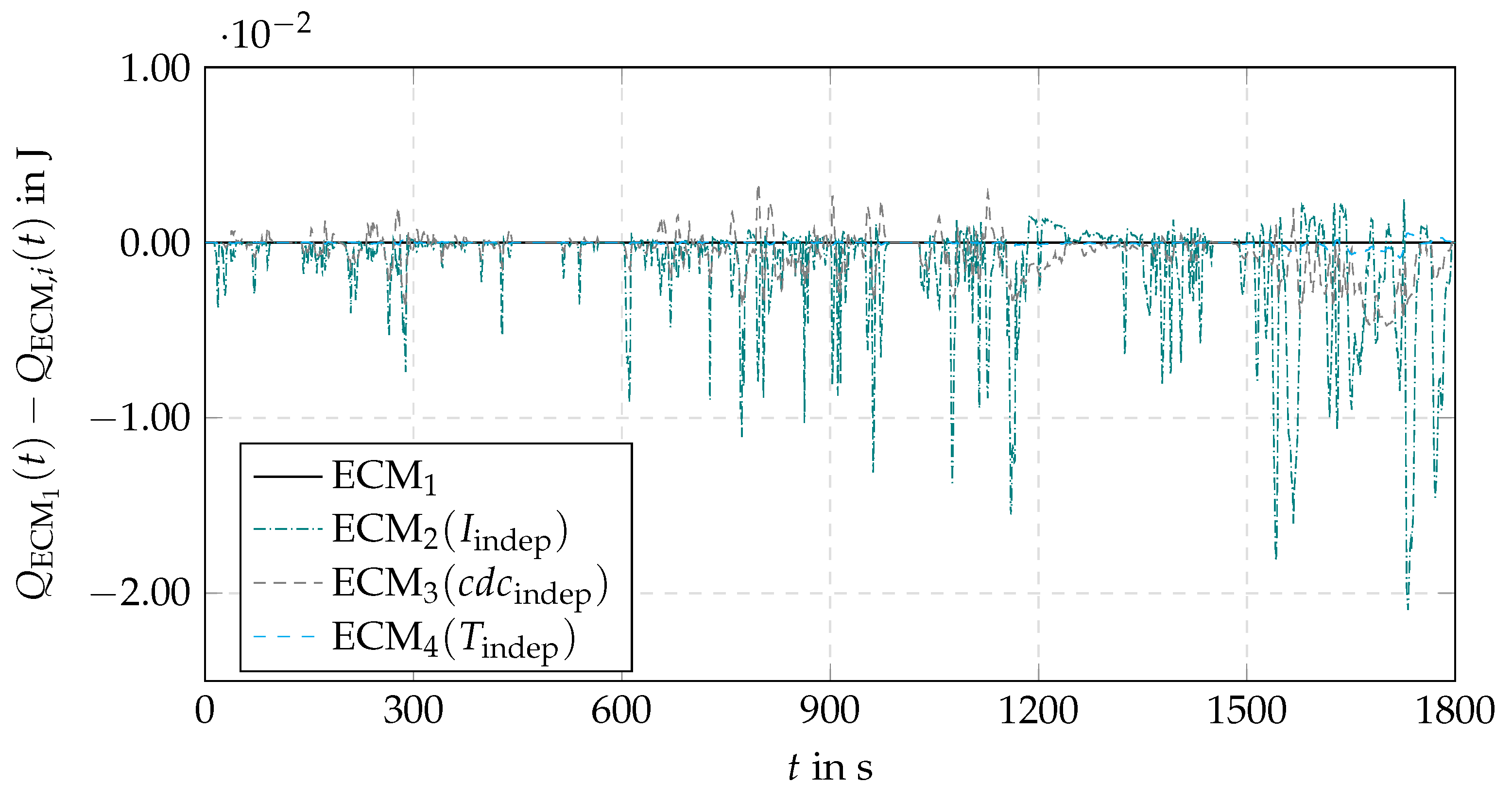
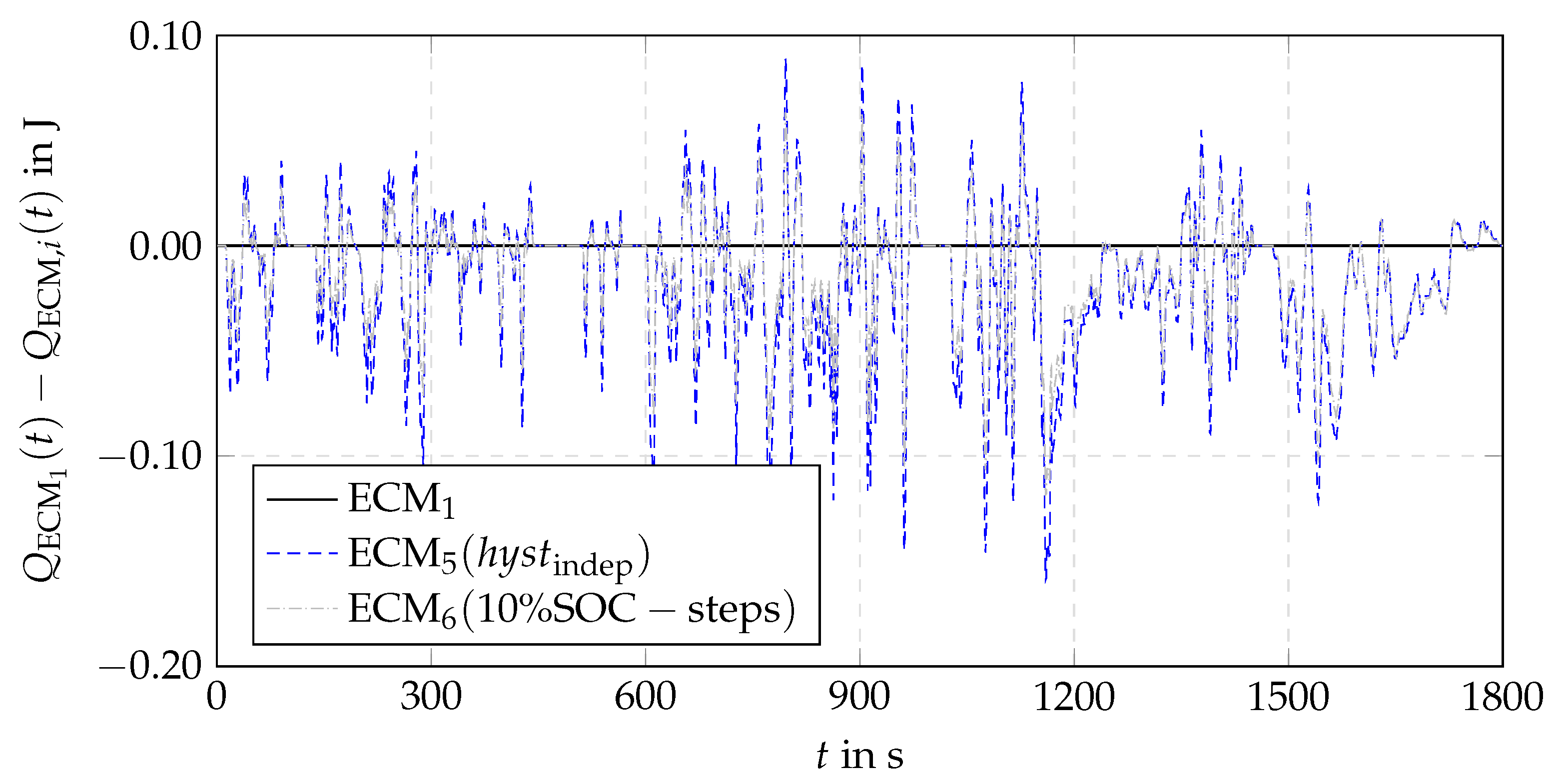
4.5. Heat Generation Comparison ECMs
4.5.1. Heat Generation Breakdown
4.5.2. ECM Comparison
5. Conclusions
Author Contributions
Funding
Data Availability Statement
Conflicts of Interest
Nomenclature
| Latin symbols | |
| A | Area () |
| Specific Heat Capacity () | |
| Charge/Discharge Pulse Dependency (−) | |
| C | C-Rate Lithium-Ion-Battery (−) |
| C | Capacitance () |
| Nominal Capacity () | |
| d | Diameter () |
| Error (%) | |
| h | Heat Transfer Coefficient () |
| Hysteresis Dependency (−) | |
| I | Current (A) |
| k | Heat Conductivity () |
| L | Length (m) |
| m | Mass (kg) |
| Nusselt Number (−) | |
| Prandtl Number (−) | |
| Q | Total Charge (A h) |
| Q | Heat (J) |
| Heat Generation Rate (W) | |
| R | Electrial Resistance () |
| Ohmic Resistance () | |
| Rayleigh Number (−) | |
| Previous State of Charge (−) | |
| t | Time (s) |
| T | Temperature (K) |
| U | Voltage (V) |
| V | Volume () |
| Greek Symbols | |
| Emissivity (−) | |
| Coulombic Efficiency (−) | |
| Density () | |
| Stefan-Boltzmann-Constant () | |
| Time Constant (s) | |
| Subscripts | |
| amb | Ambient |
| cell | Lithium-Ion-Battery Cell |
| conv | Heat Convection |
| exp | Experimentally |
| end | End Time |
| i | Counting Variable |
| indep | Independent |
| irr | Irreversible Losses |
| mean | Mean Error |
| mix | Mixing Enthalpy Losses |
| OCV | Open Circuit Voltage |
| pulse | Current Pulse |
| rad | Heat Radiation |
| reac | Side Reaction Losses |
| rel | Relaxation Time |
| rest | Rest Time |
| rev | Reversible Losses |
| t | Terminal Voltage |
| Abbreviations | |
| BEV | Battery Electric Vehicle |
| CCM | Constant Current Test Method |
| DP | Dual Polarization Model |
| EC | Entropic Coefficient Test Method |
| ECM | Electrical Equivalent Circuit Model |
| EIS | Electrical Impedance Spectroscopy |
| HPPC | High Pulse Power Characterization |
| LIB | Lithium-Ion-Battery |
| LUT | Look-Up Tables |
| OCV | Open Circuit Voltage |
| RC | Resistance-Capacitance |
| RM | Relaxation Test Method |
| SOC | State Of Charge |
| SOH | State Of Health |
| WLTC | World Harmonized Light Vehicle Test Cycle |
Appendix A


| Temperature in °C | Experimental Start SOC | Start SOC | Start SOC | Start SOC | Start SOC |
|---|---|---|---|---|---|
| 15 | 0.250 | 0.239 | 0.255 | 0.213 | 0.225 |
| 15 | 0.500 | 0.502 | 0.508 | 0.491 | 0.502 |
| 15 | 0.750 | 0.752 | 0.758 | 0.745 | 0.745 |
| 25 | 0.250 | 0.241 | 0.241 | 0.213 | 0.222 |
| 25 | 0.500 | 0.500 | 0.500 | 0.489 | 0.500 |
| 25 | 0.750 | 0.753 | 0.753 | 0.746 | 0.745 |
| 35 | 0.250 | 0.245 | 0.247 | 0.218 | 0.227 |
| 35 | 0.500 | 0.501 | 0.505 | 0.491 | 0.501 |
| 35 | 0.750 | 0.753 | 0.755 | 0.747 | 0.746 |


References
- European Union. Fit for 55. 2022. Available online: https://www.bundesregierung.de/breg-de/themen/europa/fit-for-55-eu-1942402 (accessed on 18 October 2022).
- Jouhara, H.; Khordehgah, N.; Serey, N.; Almahmoud, S.; Lester, S.P.; Machen, D.; Wrobel, L. Applications and thermal management of rechargeable batteries for industrial applications. Energy 2019, 170, 849–861. [Google Scholar] [CrossRef]
- Liu, J.; Duan, Q.; Ma, M.; Zhao, C.; Sun, J.; Wang, Q. Aging mechanisms and thermal stability of aged commercial 18650 lithium ion battery induced by slight overcharging cycling. J. Power Sources 2020, 445, 227263. [Google Scholar] [CrossRef]
- Hussein, A.A. Experimental modeling and analysis of lithium-ion battery temperature dependence. In Proceedings of the 2015 IEEE Applied Power Electronics Conference and Exposition (APEC), Charlotte, NC, USA, 15–19 March 2015; pp. 1084–1088. [Google Scholar]
- Waldmann, T.; Wilka, M.; Kasper, M.; Fleischhammer, M.; Wohlfahrt-Mehrens, M. Temperature dependent ageing mechanisms in Lithium-ion batteries—A Post-Mortem study. J. Power Sources 2014, 262, 129–135. [Google Scholar] [CrossRef]
- Lu, Z.; Yu, X.; Wei, L.; Cao, F.; Zhang, L.; Meng, X.; Jin, L. A comprehensive experimental study on temperature-dependent performance of lithium-ion battery. Appl. Therm. Eng. 2019, 158, 113800. [Google Scholar] [CrossRef]
- Pesaran, A.A. Battery thermal models for hybrid vehicle simulations. J. Power Sources 2002, 110, 377–382. [Google Scholar] [CrossRef]
- Plett, G.L. Battery Management Systems, Volume I: Battery Modeling; Artech House: Norwood, MA, USA, 2015. [Google Scholar]
- Nejad, S.; Gladwin, D.; Stone, D. A systematic review of lumped-parameter equivalent circuit models for real-time estimation of lithium-ion battery states. J. Power Sources 2016, 316, 183–196. [Google Scholar] [CrossRef]
- Wang, Q.K.; He, Y.J.; Shen, J.N.; Ma, Z.F.; Zhong, G.B. A unified modeling framework for lithium-ion batteries: An artificial neural network based thermal coupled equivalent circuit model approach. Energy 2017, 138, 118–132. [Google Scholar] [CrossRef]
- Zhang, X.; Zhang, W.; Lei, G. A review of li-ion battery equivalent circuit models. Trans. Electr. Electron. Mater. 2016, 17, 311–316. [Google Scholar] [CrossRef]
- Bernardi, D.; Pawlikowski, E.; Newman, J. A general energy balance for battery systems. J. Electrochem. Soc. 1985, 132, 5. [Google Scholar] [CrossRef]
- Wildfeuer, L.; Wassiliadis, N.; Reiter, C.; Baumann, M.; Lienkamp, M. Experimental characterization of Li-ion battery resistance at the cell, module and pack level. In Proceedings of the 2019 Fourteenth International Conference on Ecological Vehicles and Renewable Energies (EVER), Monte-Carlo, Monaco, 8–10 May 2019; pp. 1–12. [Google Scholar]
- Behi, H.; Karimi, D.; Jaguemont, J.; Gandoman, F.H.; Kalogiannis, T.; Berecibar, M.; Van Mierlo, J. Novel thermal management methods to improve the performance of the Li-ion batteries in high discharge current applications. Energy 2021, 224, 120165. [Google Scholar] [CrossRef]
- Liang, Z.; Wang, R.; Malt, A.H.; Souri, M.; Esfahani, M.; Jabbari, M. Systematic evaluation of a flat-heat-pipe-based thermal management: Cell-to-cell variations and battery ageing. Appl. Therm. Eng. 2021, 192, 116934. [Google Scholar] [CrossRef]
- Alihosseini, A.; Shafaee, M. Experimental study and numerical simulation of a Lithium-ion battery thermal management system using a heat pipe. J. Energy Storage 2021, 39, 102616. [Google Scholar] [CrossRef]
- Qian, Z.; Li, Y.; Rao, Z. Thermal performance of lithium-ion battery thermal management system by using mini-channel cooling. Energy Convers. Manag. 2016, 126, 622–631. [Google Scholar] [CrossRef]
- Cao, R.; Zhang, X.; Yang, H. Prediction of the Heat Generation Rate of Lithium-Ion Batteries Based on Three Machine Learning Algorithms. Batteries 2023, 9, 165. [Google Scholar] [CrossRef]
- Pang, H.; Wu, L.; Liu, J.; Liu, X.; Liu, K. Physics-informed neural network approach for heat generation rate estimation of lithium-ion battery under various driving conditions. J. Energy Chem. 2023, 78, 1–12. [Google Scholar] [CrossRef]
- Wu, L.; Liu, K.; Liu, J.; Pang, H. Evaluating the heat generation characteristics of cylindrical lithium-ion battery considering the discharge rates and N/P ratio. J. Energy Storage 2023, 64, 107182. [Google Scholar] [CrossRef]
- Liu, J.; Huang, Z.; Sun, J.; Wang, Q. Heat generation and thermal runaway of lithium-ion battery induced by slight overcharging cycling. J. Power Sources 2022, 526, 231136. [Google Scholar] [CrossRef]
- Catenaro, E.; Onori, S. Experimental data of lithium-ion batteries under galvanostatic discharge tests at different rates and temperatures of operation. Data Brief 2021, 35, 106894. [Google Scholar] [CrossRef]
- Kim, Y.S. Product Specifications Rechargeable Lithium Ion Battery Model: INR21700 M50 18.20Wh. 2016. Available online: https://www.dnkpower.com/wp-content/uploads/2019/02/LG-INR21700-M50-Datasheet.pdf (accessed on 18 October 2022).
- He, H.; Xiong, R.; Fan, J. Evaluation of lithium-ion battery equivalent circuit models for state of charge estimation by an experimental approach. Energies 2011, 4, 582–598. [Google Scholar] [CrossRef]
- Hu, X.; Li, S.; Peng, H. A comparative study of equivalent circuit models for Li-ion batteries. J. Power Sources 2012, 198, 359–367. [Google Scholar] [CrossRef]
- Ng, K.S.; Moo, C.S.; Chen, Y.P.; Hsieh, Y.C. Enhanced coulomb counting method for estimating state-of-charge and state-of-health of lithium-ion batteries. Appl. Energy 2009, 86, 1506–1511. [Google Scholar] [CrossRef]
- Spotnitz, R.; Franklin, J. Abuse behavior of high-power, lithium-ion cells. J. Power Sources 2003, 113, 81–100. [Google Scholar] [CrossRef]
- Thomas, K.E.; Newman, J. Thermal modeling of porous insertion electrodes. J. Electrochem. Soc. 2003, 150, A176. [Google Scholar] [CrossRef]
- Siemens, P. STAR-CCM+ User Guide Version 13.04; Siemens PLM Software Inc.: Munich, Germany, 2022. [Google Scholar]
- Immonen, E.; Hurri, J. Incremental thermo-electric CFD modeling of a high-energy Lithium-Titanate Oxide battery cell in different temperatures: A comparative study. Appl. Therm. Eng. 2021, 197, 117260. [Google Scholar] [CrossRef]
- Klan, H. Wärmeübergang durch freie Konvektion an umströmten Körpern. In VDI-Wärmeatlas; Springer: Berlin/Heidelberg, Germany, 2002; pp. 567–591. [Google Scholar]
- Stephan, P. B2 Grundlagen der Berechnungsmethoden für Wärmeleitung, konvektiven Wärmeübergang und Wärmestrahlung. In VDI-Wärmeatlas; Springer: Berlin/Heidelberg, Germany, 2019; pp. 23–36. [Google Scholar]
- Basytec. Battery Cell and Module Test System. 2017. Available online: https://basytec.de/prospekte/2023_01_BaSyTec%20MRS.pdf (accessed on 18 October 2022).
- Nikolian, A.; Jaguemont, J.; De Hoog, J.; Goutam, S.; Omar, N.; Van Den Bossche, P.; Van Mierlo, J. Complete cell-level lithium-ion electrical ECM model for different chemistries (NMC, LFP, LTO) and temperatures (- 5 C to 45 C)–Optimized modelling techniques. Int. J. Electr. Power Energy Syst. 2018, 98, 133–146. [Google Scholar] [CrossRef]
- Belt, J.R. Battery Test Manual for Plug-in Hybrid Electric Vehicles; Technical Report; Idaho National Lab. (INL): Idaho Falls, ID, USA, 2010. [Google Scholar]
- Schmidt, J.P. Verfahren zur Charakterisierung und Modellierung von Lithium-Ionen Zellen; KIT Scientific Publishing: Karlsruhe, Germany, 2013; Volume 25. [Google Scholar]
- Geifes, F.; Bolsinger, C.; Mielcarek, P.; Birke, K.P. Determination of the entropic heat coefficient in a simple electro-thermal lithium-ion cell model with pulse relaxation measurements and least squares algorithm. J. Power Sources 2019, 419, 148–154. [Google Scholar] [CrossRef]
- Forgez, C.; Do, D.V.; Friedrich, G.; Morcrette, M.; Delacourt, C. Thermal modeling of a cylindrical LiFePO4/graphite lithium-ion battery. J. Power Sources 2010, 195, 2961–2968. [Google Scholar] [CrossRef]
- Zhu, Q.; Xiong, N.; Yang, M.L.; Huang, R.S.; Hu, G.D. State of charge estimation for lithium-ion battery based on nonlinear observer: An H∞ method. Energies 2017, 10, 679. [Google Scholar] [CrossRef]
- Geng, Z.; Groot, J.; Thiringer, T. A time-and cost-effective method for entropic coefficient determination of a large commercial battery cell. IEEE Trans. Transp. Electrif. 2020, 6, 257–266. [Google Scholar] [CrossRef]
- Steinhardt, M.; Gillich, E.I.; Rheinfeld, A.; Kraft, L.; Spielbauer, M.; Bohlen, O.; Jossen, A. Low-effort determination of heat capacity and thermal conductivity for cylindrical 18650 and 21700 lithium-ion cells. J. Energy Storage 2021, 42, 103065. [Google Scholar] [CrossRef]
- Bui, T.M.; Niri, M.F.; Worwood, D.; Dinh, T.Q.; Marco, J. An Advanced Hardware-in-the-Loop Battery Simulation Platform for the Experimental Testing of Battery Management System. In Proceedings of the 2019 23rd International Conference on Mechatronics Technology (ICMT), Salerno, Italy, 23–26 October 2019; pp. 1–6. [Google Scholar]
- Lambert, F. Tesla Model 3: Exclusive First Look at Tesla’s New Battery Pack Architecture. 2017. Available online: https://electrek.co/2017/08/24/tesla-model-3-exclusive-battery-pack-architecture/ (accessed on 18 October 2022).


| Dependent | Independent | |
|---|---|---|
| I | LUTs for every tested current pulse value | LUT for optimized value of all tested current pulses |
| LUTs separately for charge and discharge pulses | LUT for optimized value of both charge and discharge pulses | |
| LUTs for charge OCV and discharge OCV | LUT taking the arithmetic middle between charge and discharge OCV | |
| T | LUTs for all conducted test temperatures | LUT only for = 25 °C |
| Nominal Capacity in mA h | |||
|---|---|---|---|
| 5 °C | 25 °C | 45 °C | |
| LG 21700 | 4590 | 4800 | 4720 |
| Open Circuit Voltage | Ohmic Resistance | Resistance/Capacitance / | Resistance/Capacitance / | SOC Data Points | |
|---|---|---|---|---|---|
| f(SOC,T,) | f(SOC,T,cdc,I) | f(SOC,T,cdc,I) | f(SOC,T,cdc,I) | 5% steps | |
| f(SOC,T,) | f(SOC,T,cdc) | f(SOC,T,cdc) | f(SOC,T,cdc) | 5% steps | |
| f(SOC,T,) | f(SOC,T,I) | f(SOC,T,I) | f(SOC,T,I) | 5% steps | |
| f(SOC,) | f(SOC,cdc,I) | f(SOC,cdc,I) | f(SOC,cdc,I) | 5% steps | |
| f(SOC,T) | f(SOC,T,cdc,I) | f(SOC,T,cdc,I) | f(SOC,T,cdc,I) | 5% steps | |
| f(SOC,T,) | f(SOC,T,cdc,I) | f(SOC,T,cdc,I) | f(SOC,T,cdc,I) | 10% steps | |
| f(SOC,T,) | f(SOC,T,cdc,I) | f(SOC,T,cdc,I) | - | 5% steps | |
| f(SOC,T,) | f(SOC,T,cdc,I) | - | - | 5% steps |
Disclaimer/Publisher’s Note: The statements, opinions and data contained in all publications are solely those of the individual author(s) and contributor(s) and not of MDPI and/or the editor(s). MDPI and/or the editor(s) disclaim responsibility for any injury to people or property resulting from any ideas, methods, instructions or products referred to in the content. |
© 2023 by the authors. Licensee MDPI, Basel, Switzerland. This article is an open access article distributed under the terms and conditions of the Creative Commons Attribution (CC BY) license (https://creativecommons.org/licenses/by/4.0/).
Share and Cite
Auch, M.; Kuthada, T.; Giese, S.; Wagner, A. Influence of Lithium-Ion-Battery Equivalent Circuit Model Parameter Dependencies and Architectures on the Predicted Heat Generation in Real-Life Drive Cycles. Batteries 2023, 9, 274. https://doi.org/10.3390/batteries9050274
Auch M, Kuthada T, Giese S, Wagner A. Influence of Lithium-Ion-Battery Equivalent Circuit Model Parameter Dependencies and Architectures on the Predicted Heat Generation in Real-Life Drive Cycles. Batteries. 2023; 9(5):274. https://doi.org/10.3390/batteries9050274
Chicago/Turabian StyleAuch, Marcus, Timo Kuthada, Sascha Giese, and Andreas Wagner. 2023. "Influence of Lithium-Ion-Battery Equivalent Circuit Model Parameter Dependencies and Architectures on the Predicted Heat Generation in Real-Life Drive Cycles" Batteries 9, no. 5: 274. https://doi.org/10.3390/batteries9050274