

Fly by Feel: Flow Event Detection via Bioinspired Wind-Hairs

Department of Engineering, City, University of London, Northampton Square, London EC1V 0HB, UK
*
Author to whom correspondence should be addressed.
Fluids 2024, 9(3), 74; https://doi.org/10.3390/fluids9030074
Submission received: 31 January 2024
/
Revised: 7 March 2024
/
Accepted: 13 March 2024
/
Published: 15 March 2024
(This article belongs to the Special Issue Fluid Dynamics in Biological, Bio-Inspired, and Environmental Systems)
Abstract
:Bio-inspired flexible pillar-like wind-hairs show promise for the future of flying by feel by detecting critical flow events on an aerofoil during flight. To be able to characterise specific flow disturbances from the response of such sensors, quantitative PIV measurements of such flow-disturbance patterns were compared with sensor outputs under controlled conditions. Experiments were performed in a flow channel with an aerofoil equipped with a 2D array of such sensors when in uniform inflow conditions compared to when a well-defined gust was introduced upstream and was passing by. The gust was generated through the sudden deployment of a row of flaps on the suction side of a symmetric wing that was placed upstream of the aerofoil with the sensors. The resulting flow disturbance generated a starting vortex with two legs, which resembled a horseshoe-type vortex shed into the wake. Under the same tunnel conditions, PIV measurements were taken downstream of the gust generator to characterise the starting vortex, while further measurements were taken with the sensing pillars on the aerofoil in the same location. The disturbance pattern was compared to the pillar response to demonstrate the potential of flow-sensing pillars. It was found that the pillars could detect the arrival time and structural pattern of the flow disturbance, showing the characteristics of the induced flow field of the starting vortex when passing by. Therefore, such sensor arrays can detect the “footprint” of disturbances as temporal and spatial signatures, allowing us to distinguish those from others or noise.
1. Introduction
In the natural world, it can be seen that many animals and insects have a variety of ‘in-built’ sensors, which they can use for flight sensing or event detection in both air and water. Bats are one example; they have hair-like structures that coat their wings, which have been the subject of in-depth research. Ref. [1] hypothesised and found that bats use these hairs to sense changes in the boundary layer profile to improve their stability and manoeuvrability during flight. Similarly, Ref. [2] found that the wind-hairs had high sensitivity to reverse airflow to allow bats to monitor instabilities during slow flight that could lead to separation. It should also be noted that bats are incredibly complex fliers, and their wings contain many features that improve their performance [3]; therefore, they rely on such sensors to remain in full control during extreme manoeuvrability. It is not only bats that possess these sensing hairs; seals also use sensing whiskers [4], through which the oncoming flow direction and velocity can be felt according to the dynamic responses of their whiskers. Rats are thought to have active whisker sensing abilities [5]; they may be able to control the relative velocities of their whiskers when using them to sense surfaces in their surroundings. This is an area of nature from which aviation can benefit once flying by feel can be realised, as tactile whiskers have already proven that learning from these designs is useful [6,7].
Many researchers are developing and testing bio-inspired sensors for a variety of applications in engineering. A good overview can be found in the review papers by [8] and the most recent one by [9]. Such sensors have been developed based on optical, piezoresistive, piezoelectric, and capacitive principles. With respect to air flows, optical sensors were developed by the authors of [10] in the form of flexible microscopic cantilever beam sensors for wall shear stress measurements, and they allowed the optical detection of separation in complex turbulent flows. Other research has been performed on sensors that can sense very low-speed air flow with directional sensitivity [11]. Research has also been performed on piezoresistive hair-like sensors specifically for airflow sensing [12], and the results showed that the response was proportional to the oncoming airflow velocity. Work such as that of [13] developed flexible skin for an NACA0012 by mimicking biological systems. The flexible sensing skin could measure surface pressure, temperature, and wall shear stress and has the potential to improve the capabilities that UAVs have both aerially and underwater. There is current interest in underwater MEMS sensors for applications such as underwater autonomous vehicles [14,15,16]; the natural inspiration for these sensors tends to be fish that live in areas of very low light that have to rely on sensors for their surroundings. Ref. [17] developed and tested high-sensitivity neuromast-inspired flow sensors based on biological sensors that blind cavefish have for the navigation of underwater robots. On the other hand, Ref. [18] developed and tested sensors on a biomimetic robotic stingray, and the sensors were successfully used to provide inputs to the robot that allowed it to track a given trajectory. In that sense, a fly-by-feel flight system based on bio-inspired hair sensors could improve the safety and reliability of flight manoeuvres in complex environments. In addition, such sensor arrays could also be useful for aerodynamic design studies in wind and water tunnels or for proving computational models.
In our lab, nature-inspired flexible pillar structures were developed as biomimetic wind-hairs and have already proven their ability for flow event detection and incipient stall monitoring ([19]). These flexible pillar sensors work on the principles of flexible cantilever beams that are deflected by flow-induced drag forces and, as such, allow the detection of flow events by optically monitoring their dynamic behaviour. Similar strategies were also developed and reviewed for underwater flow sensing based on seal whiskers [20,21,22]. One benefit of such sensing systems is the potential for implementing these sensors in flow control strategies, which, overall, would allow reactions to critical flow situations through preventive measures, e.g., preventing stall after sensing premature instabilities along the wing. In nature, we can see the benefits of morphing wings that can react to gusts or unstable flight conditions. Research has been performed on the wing-morphing ability of peregrine falcons during dive and pull-out manoeuvres [23], thus improving their manoeuvrability in certain flight conditions. Wing-morphing action can optimise drag performance in specific situations and mitigate stall [6]. Furthermore, active flow control is possible through distributed flaplets on the wing and trailing edge—that is, leading and trailing edge morphability [24]. Such distributed flaplets can help to control the distribution of circulation and drag along the span in a sensitive way. Such a wing was designed in our lab [25], and the individually controllable flaplets mimicked the pop-up feathers that birds have. This concept has been used as a disturbance generator in which the flaplets open and close to create a gust-like disturbance, and it will be used in such a way again here. Integrating the sensors on the same wing paves the way for in-built flow monitoring, which could enable circulation management via feedback control through continuous flow monitoring. Such real-time feedback is possible through the advent of highly sensitive motion-tracking cameras or event-based cameras, which offer real-time flow monitoring of optical sensors.
This paper is structured as follows: After the introduction, the second section details the experimental methods and the modification of a wing with actuated flaplets. The sensing principle is explained, and the integration of the sensors on an NACA0012 aerofoil is shown. The results of the experiments in uniform flow and with an induced gust are presented by means of the velocity fields and the response of the sensor array. A discussion and concluding remarks are given at the end.
2. Materials and Methods
All experiments were performed in the low-speed water tunnel at the City University of London. The tunnel was an open surface and had a clear test section with a length of 1.5 m at a cross-section of 40 cm by 40 cm. Comparing similar Reynolds numbers, performing flow studies in a water tunnel as opposed to a wind tunnel allowed for lower-budget experimental equipment but yielded higher-quality PIV images. The typical flow speeds used were 35 cm/s at a chord-based Reynolds number of 100 k.
2.1. Disturbance Generation
The disturbance generation was realised with a symmetric NACA0012 wing (chord C1 = 30 cm) with four individually controlled pneumatically actuated flaplets, as previously developed in [25]. The pneumatic actuation was since updated from balloons to small pneumatic cartridge cylinders to overcome past repeatability concerns. The cartridges were from Festo (EGZ-6-5 Pneumatic Piston Rod Cylinder, Single Acting).
As shown in Figure 1, the disturbance model was connected to a high-pressure air source and then regulated down to the required operating pressure of the actuators of 2 bar. The flaplets were easily controlled via an Arduino board, the different buttons of which could be programmed to operate different flaplet duty cycles by opening and closing the valves.
The flaplets had a clear rectangular section of a thin acrylic sheet stuck on the suction side to ensure that there was a smooth and continuous flow surface. Figure 2 shows the middle four flaps when open. For the generation of the gust disturbance, the four consecutive flaplets shown were opened, held for 1 s, and then closed, with opening and closing phases that lasted around 250 ms. The generated gust had the form of a starting vortex, which was shed from the trailing edge once the flaps had reached their maximum deployment position. A further description of the vortex was gained from PIV measurements.
2.2. Experimental Setup for PIV
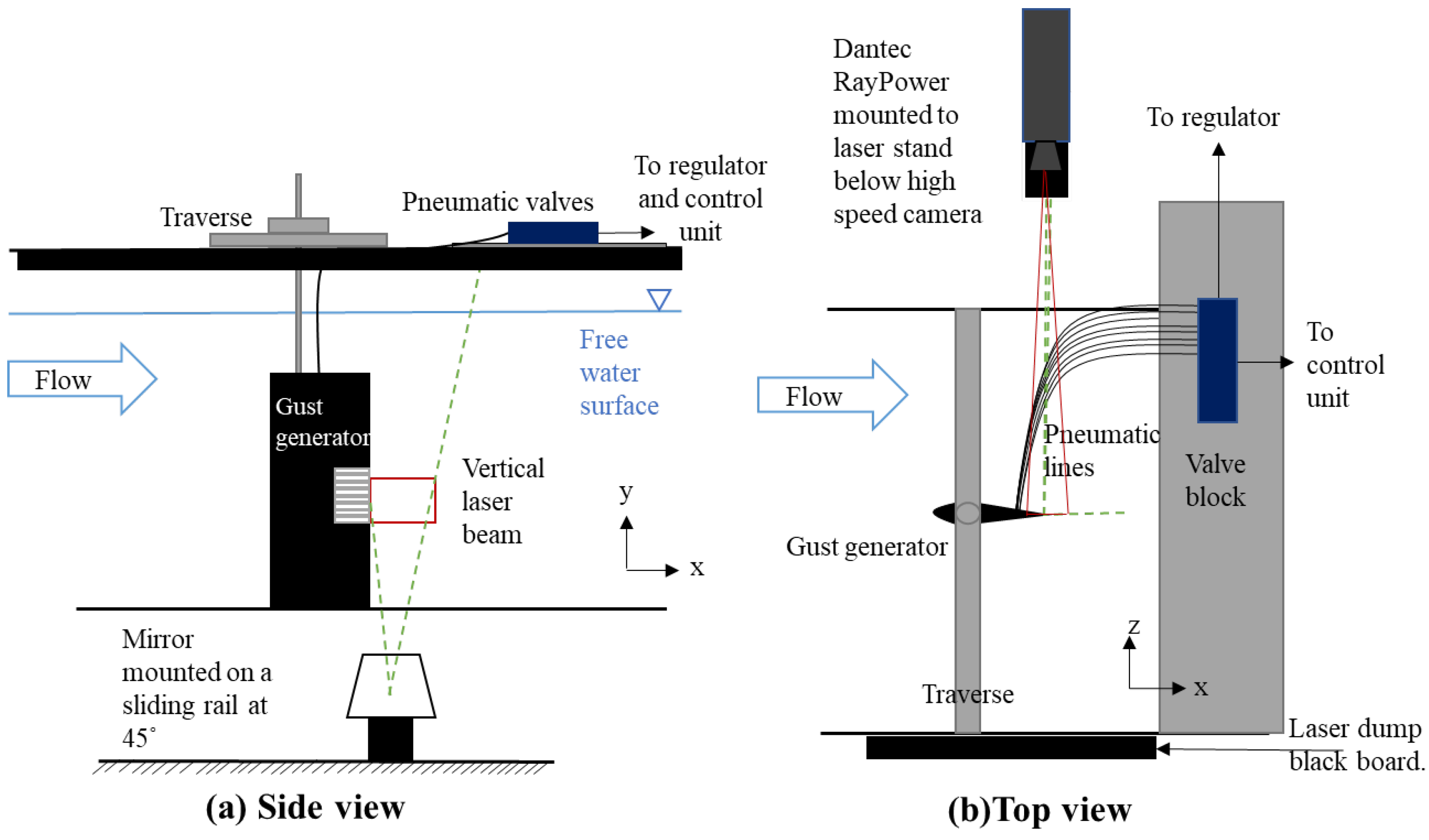
The disturbance generator model explained above was set up in the tunnel such that the free ends of the model were against the lower viewing window of the test section and out of the tunnel at the free surface. The model was placed in the tunnel’s centre to avoid wall effects. The flaplets are also centred in the channel flow to avoid the lower wall effects and the upper wave effects from the open surface. The camera used for all measurements was a high-speed Phantom M30, and the required section was illuminated with a Dantec raypower 5000 5W continuous-wave argon-ion laser ( = 532 nm) with a sheet thickness of 1 mm. Using a Tokina 100 mm macro lens, the frame rate of the camera was a continuous 700 fps, and it had an f-value of 2.8 with an exposure time of 1430 s and a window size of 1280 × 800.
To capture the disturbance generated in detail, two PIV setups were arranged. The first was with the light-sheet oriented in the horizontal plane, crossing the disturbance generator in the middle of the flap row that was to be actuated. The second setup used the light-sheet in the vertical plane, parallel to the suction side and in line with the trailing edge. For both setups, two sets of images were captured—the first at the trailing edge and the second at a half chord (15 cm) further downstream. This was achieved via a traverse to which the gust generator model was attached, while the recording setup remained in its position. A pre-mixed solution of tracer particles (diameter: 50 m) was added to the tunnel and allowed to mix thoroughly for an even seeding. Below, Figure 3 shows the vertical plane setup for PIV measurements, the green dashed lines represent the approximated edges of the laser sheet and the red lines show the approximated field of view to the camera.
2.3. PIV Processing
The recorded time series were processed using a PIV processing toolbox that was developed in-house and was written in Matlab. The code used the 2D cross-correlation between pairs of successive images in the time series. The time separation of the images was equal to the inverse of the recording frequency (700 fps). A multi-pass algorithm that ran over two iterations across the images in small, decreasing interrogation windows with window refinement (1st iteration: 48 × 48 pixels, second iteration: 32 × 32 pixels) was used. The correlation peak was fitted with a three-point Gaussian curve in the x- and y-directions to achieve sub-pixel accuracy. The typical mean velocities resulted in displacements of between three and four pixels. Erroneous vectors were filtered out using the maximum and minimum ranges of the expected velocities and a local median filter. The vectors from those positions were interpolated from the nearest neighbours. A final 3 × 3 kernel Gaussian smoothing filter was run over the results to remove small-scale structures, highlighting large-scale coherent motion patterns.
2.4. Sensing Pillars
Work was previously carried out by our team to develop and calibrate flexible pillar sensors in boundary layers down to a wall distance of 300 microns, where they acted as wall shear stress sensors ([19,26]). These sensors followed the principle of a one-sided clamped cantilever beam that was bent by drag forces from the flow around the pillar. The measured signal was the tip bending between the wind-off and the wind-on situation. If the length of the pillar was small enough such that it was fully submerged in the viscous sublayer of the near-wall flow boundary, then this measure was proportional to the wall shear, as the load profile was linear along the structure. With their slender filamentous shape, these pillars mimicked sensors seen in the natural world, such as wind-hairs on bats [2], and they have proven useful for the detection of flow events. Therein, the length was of the order of the boundary layer thickness, which then integrated the forces along the length of the sensor in a nonlinear manner. Therefore, the response was first-order proportional to the mean velocity at the edge of the boundary layer but was also affected by the changes in the curvature of the velocity profile ([1]). As shown in our previous work, the response of such sensors closely followed that of a second-order harmonic oscillator, which was described by a nearly constant gain until 30 percent of the natural frequency . In liquids, the response is typically overdamped, and this excludes any ringing ([26]).
The methodology presented herein followed the design of such sensors to be implemented in complex geometries by using the technique of planar inlays made of elastomeric sheets. These pillars were easily laser-cut from the large elastomeric sheets (sheet thickness: 1.5 mm) and then clamped between parts of the model, as shown in [19,26]. The shape of the elastomeric sheet was based on the wing cross-section and also had protuberances in the form of long slender beams with rectangular cross-sections, which represented the biomimetic sensory hairs. A wing model based on an NACA0012 profile that had an integrated 2D array of such sensors on the suction side was built. Each row of sensing pillars was clamped between the NACA0012 model sections. Each silicone section was an NACA0012 base with a 20 cm chord and six evenly spaced pillars, starting at 15% of the chord. The pillars had a length of 7 mm and a rectangular cross-section of 1.5 mm by 0.3 mm, with the longer side being perpendicular to the freestream flow direction. This made the pillars bend predominantly in the streamwise flow direction, and they were not sensitive to spanwise flow; see Figure 4.
The method of calibrating the sensors was described in detail in [19]. The static response was about a 1 mm tip deflection per velocity increase of 5 m/s. The natural frequency of the structures in water was approximately 17 Hz. Note that these values depended on the Young modulus of the elastomeric material and the clamping conditions, which needed careful control during the calibration process and the measurements. This was because these conditions could vary with time or the handling of the wing model.
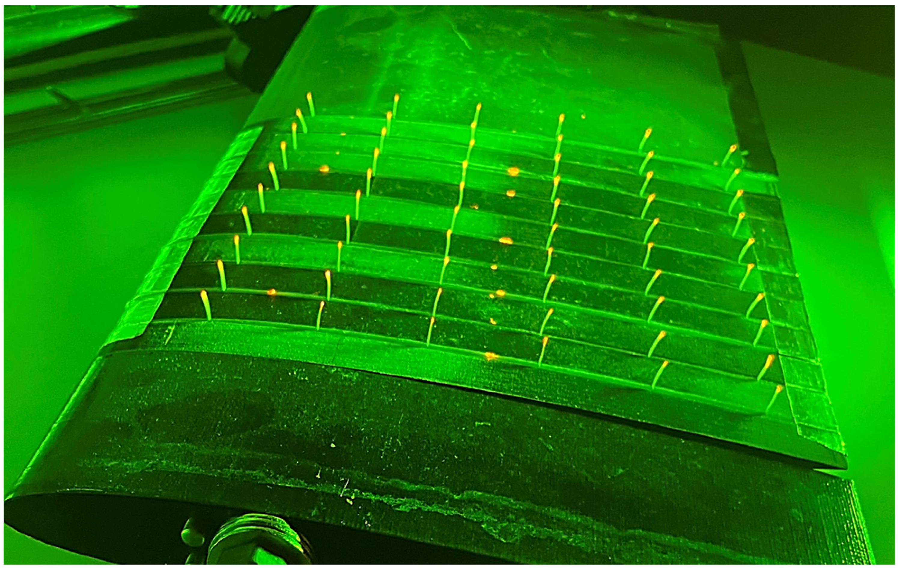
Figure 5 shows the pillars under a green LED light, with the pink tips highly visible. The tips of the pillars were carefully marked with fluorescent dye (MMA-RhB- 113 Frak-Paticles, Dantec Dynamics, 584 nm peak emission, 540 nm peak absorption) to enhance the tip movement and aid in tracking them effectively. In Figure 5, dye spots marked on the model can also be seen; these were to ensure that the model did not move during the tests, and they were used as reference spots.
2.5. Experimental Setup for Pillar Tracking
The NACA0012 wing equipped with the sensing pillars was placed downstream of the disturbance generator, and the pillars acted as ‘wind hairs’ to sense flow disturbances.Each one of the pillar tips was marked at the tip with a dye that could be seen through a bandpass colour-filter camera lens for greater contrast. Continuous recordings were taken as the flow disturbance passed the camera viewing window to characterise the flow. The recordings were processed to obtain the pillar tip deflection along the array. An in-house MATLAB code determined the relative displacement of the marked pillar tip locations between the “wind-off” and “wind-on” situations with an accuracy of 20 microns. This accuracy was achieved by interpolating the Gaussian peak in the underlying cross-correlation procedure, as explained previously.
In Figure 6, C1 is the chord length of the gust generator (30 cm), and C2 is the chord length of the sensing wing (20 cm).
3. Results
3.1. PIV Disturbance Characterisation
The disturbance generated with the deployment of the four flaps as described in Section 2 was characterised with PIV measurements in the wake in the vertical plane along the chord of the wing (zero AoA) and in the horizontal plane crossing the centre of the deployed flaps. Figure 7 gives an impression of the PIV flow pictures after deployment, and they are shown in the style of multi-exposed images by adding a number n of 10 successive images with an inter-spacing of two images. This illustrates the flow as if the picture was made with a pulsed laser light. The top view shows the curvature of the pathlines around the outer edges of the deployed flaps, where the flow was diverted to flow around those edges. This flow pattern was nearly mirror-symmetric to the horizontal centreline in the middle of the deployed flaps. In the direct wake of the flaplets, one can see nearly stagnant flow, which then accelerated when moving further downstream. The cross-sectional view indicates the stages during deployment from the reflections of the edge of the flap. During its opening, flow was sucked into the void space, and a clockwise rotating vortex was formed underneath the trailing edge of the flap. This starting vortex grew until the flaps were stopped, which was when it was shed into the wake.
The PIV images were taken at snapshots in the flow and are shown in non-dimensionalised time as follows: where t is the time in seconds, is the freestream velocity (0.35 m/s), and C is the chord length of the gust generator (0.30 m). We considered t = 0 s and, therefore, t* = 0 to be at the point at which the flaplets became fully open. Below, in the figures, the convection of the disturbance structure can be seen as one moves from left to right. The trailing edge and flaplets were added to aid with layout understanding.
It can be seen from the diverging streamlines near the flaps in Figure 8 that there was a flow disturbance at the bottom due to the flaplets fully opening. This agreed with the flow visualisation pattern from the multi-exposed images. The grey-coloured region at a short distance downstream at time t* = 0.1 indicated a region of lower streamwise velocity in the wake, which corresponded to the region cut through the centre plane in Figure 9 at t* = 0.1. This was where the streamwise velocity was reduced due to the induction of the head of the starting vortex (indicated by the red arrow in the figure).
The patterns in Figure 8 show again for all times a certain degree of symmetry to the centreline, which let us speculate that the starting vortex was nearly symmetric to the centreline of the flaps. From fundamental vortex theory (vortex lines must close), we concluded that the vortex seen in the cross-sectional view was the head of a vortex loop that had legs in the form of the tip vortices at the edges of the outer flaps; see below.
The left-hand counterclockwise rotating red arrow indicates the motion of the flaplets opening, and the following clockwise rotating red arrow indicates the head of the vortex loop, with a region of high velocity on top and lower velocities underneath due to the velocity induction effect. Note that the vortex was convecting downstream with the mean flow; therefore, the streamlines representing the vortex were not closed in circular form but were seen as a strong bending curvature (addition of mean flow + circulation). This corresponded to the flow region representing the core of the starting vortex.
Superimposing the snapshots in both the horizontal and vertical planes allowed us to draw conclusions regarding the 3D structure of the starting vortex. A drawing of the underlying structure is sketched in Figure 10, and it resembles a horseshoe-type shape of the starting vortex when being shed into the wake. The head of the horseshoe was the front of the vortex loop, while the legs were joined on either end to the trailing vortices at the ‘wing tips’ of each of the outer flaplets. Figure 10 illustrates our understanding of the shape of the initial horseshoe vortex forming at the flaplets and then the same vortex as it shed and traveled further downstream.
3.2. Disturbance Sensing via Pillars
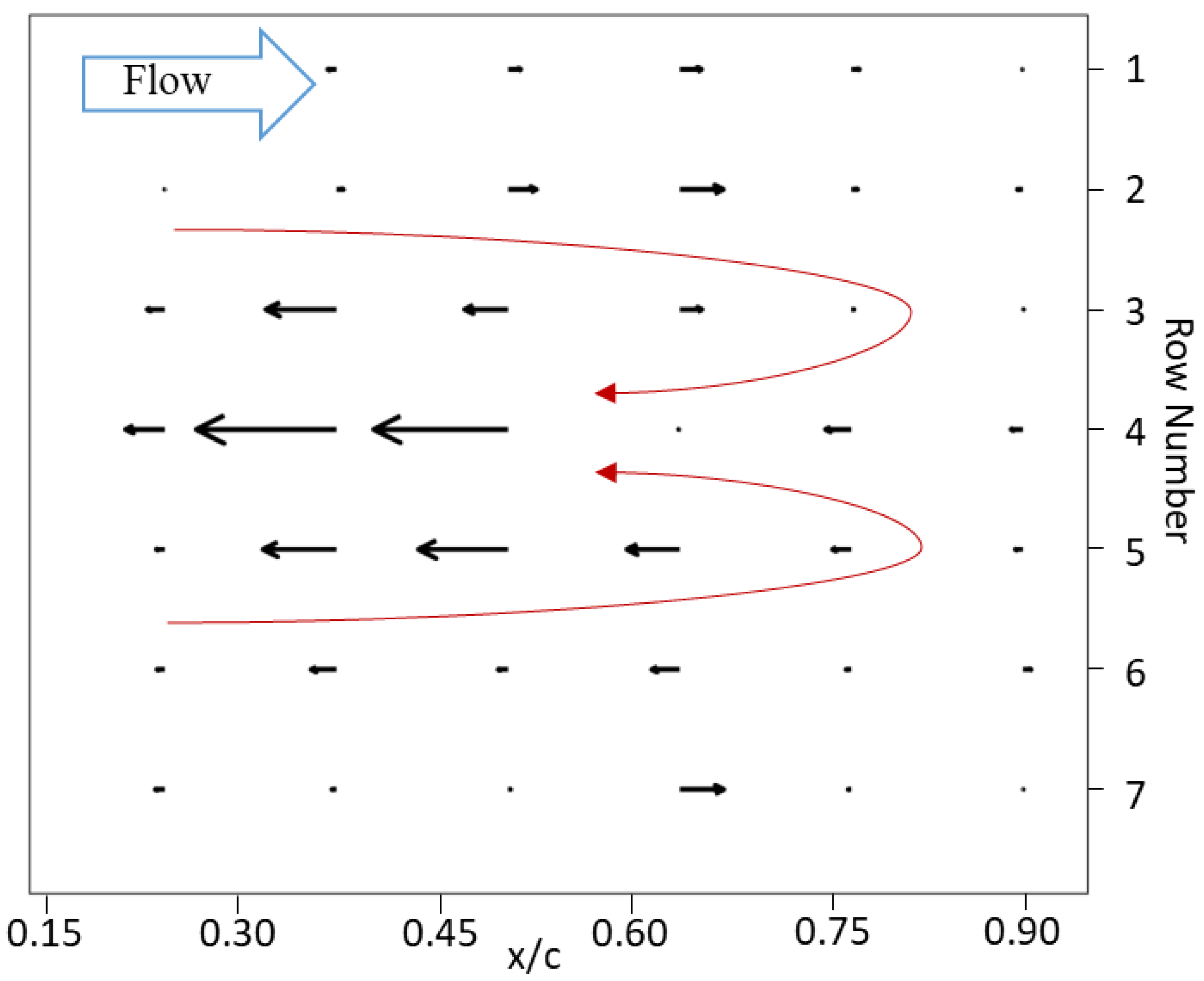
The results from the image processing of the sensor images were in the form of the pillar tip displacement along the nodes of the array for several i columns and several j rows. The tip displacement was only measured in the streamwise direction. In Figure 11, it should be noted that the peak tip displacement was four pixels, corresponding to 1 mm of tip deflection. These data were used to plot a quiver plot of the pillar tip deflections at selected times to compare the detected patterns with the induced flow disturbance. It should be noted that the quiver plot given below had the mean flow deflection subtracted to emphasise the slowing of the flow relative to the mean. Therefore, positive bending showed accelerated flow, while negative bending showed a decelerated flow, where flow is represented by the black arrows in Figure 11.
An exemplary result is shown for t* = 0.7 in Figure 11, which was when the disturbance was expected to convect to the middle of the sensory array (for the given period and distance from the gust generator). It can be seen that the disturbance roughly appeared over five pillar rows at a time (rows 2–6, as shown); this correlated well with the affected span seen in Figure 8, where the disturbance also acted over the span of the deployed flaps. In addition, the reconstructed pattern showed some degree of symmetry to the centreline, similarly to what was observed in the characterisation of the disturbance pattern. There was a maximum local reduction in the deflection of the pillars along the centreline row for columns 2 and 3 (in line with the centre of the flaps). A weaker reduction was above and below this row, which was where the pillar tips were nearer to the outer flaplets. Further away from the centreline, there was some flow acceleration, as shown by the positive bending of the pillars. The red lines overlaid on the quiver plot indicated the suggested alignment of the head of the vortex loop and the resulting induced flow pattern underneath, as expected from the PIV images. Overall, the reconstructed pattern matched with what was expected to be a footprint of the horseshoe vortex on the trailing wing. Note that the strength of the induced vortex dissipated over the travel distance between the gust generator and sensing aerofoil due to viscous diffusion. This was why the PIV measurements for characterisation were performed in the same downstream location as where the sensing pillars were placed.
The figure clearly shows that the pillars were able to detect the event according to the time and structure that it left as a footprint of the disturbance when travelling over the wing. In combination with event-based cameras or real-time image processing, such events can be recorded online, which is the pathway for feedback flow control. The observed pattern was also typical for stall cells [27]; therefore, such measurements could also help in investigating the dynamics of such flow features in research.
4. Discussion
Our focus herein was the application of imaging techniques to the detection of patterns of sensor deflections that deviate from the mean situation when an aerofoil is flying in gusty conditions. The findings and their interpretations are discussed in this section, alongside the limitations and future research.
From the results, it can be seen that the pillars detected the disturbances created by the gust generator, as both the disturbance and the quiver plot showed five rows of pillars being affected. Note again that the quiver plot that is shown plotted the tip deflection relative to the mean. The documented instantaneous pattern was nearly symmetrical to the horizontal centreline, which was the plane of symmetry of the horseshoe-type flow structure generated by the gust generator. As mentioned above, the starting vortex was generated and shed when the opening had stopped, and the structure was then travelling along the suction side of the trailing wing, which was equipped with the sensing pillars. When the starting vortex was moving above the area of the pillars, we saw flow deceleration in the centre and positive flow acceleration along the outside of the structure. This reflected the induced flow field underneath the horseshoe vortex. Therefore, the pillars were able to detect the event according to the time and structure that it left as a “footprint” of the disturbance when travelling over the wing.
Overall, the results so far represent a rather qualitative picture of the disturbance pattern. In correlating the strength of those patterns, we must assume that the bending magnitude was approximately proportional to the mean velocity in the boundary layer and that the sensor response was fast enough to respond to critical events, which was predefined by the mechanical response of the cantilever-beam-type elastic pillar. Beyond that, a further direct quantification of the flow velocities from the tip bending magnitude was not possible with good accuracy. This would require some further knowledge of the shape of the velocity profiles and details of the boundary-layer characteristics, in addition to calibration in the respective flows. As such profile details are often not known a priori, the major value under such conditions is that of gaining the spatiotemporal characteristics of a disturbance pattern, albeit probably not reflecting all details of the disturbance in frequency, scale, and strength. Nevertheless, the observed tip deflection pattern was correlated in structure, symmetry, and magnitude with the induced horseshoe-vortex-type disturbance of the flow. Therefore, modern imaging techniques such as online motion capture technologies can be applied to the tips of the sensors to help “feel” such disturbances in real time during flight.
5. Conclusions
The results provided in this study show the ability of flow-sensing pillars to be used to detect the spatiotemporal footprints of flow events passing over a wing according to tests in a flow channel with a specific gust generator. The observed pattern was also typical for stall cells [27]; therefore, such measurements can also help in the investigation of the dynamics of such flow features in research. In combination with online image motion capture techniques applied to fluorescent pillar tips, such events can be recorded online, which is the pathway for feedback flow control.
This verification of the capabilities of the pillars allows future research that uses them to be carried out. Event-based cameras are being investigated for flow monitoring, and their potential is currently being discussed in other image-based velocimetry methods, such as PIV [28]. It is hypothesised that event-based imaging of the 2D arrays of our sensor pillars would be an ideal candidate for such technology, as the objects of interest (the pillar tips) are arranged in a well-ordered pattern, and the deflections are typically in a limited range around the original wind-off situation. Furthermore, there is no need to calibrate for any out-of-plane motion, as the geometrical structure of the sensors is predominately designed to be sensitive only to flow in the streamwise direction. In addition, the given number of pillars would provide a defined number of selected markers in the flow to be monitored, as this does not change over time. This type of event-based imaging of the sensors is planned as future work in our lab. Furthermore, machine learning may help train the system for specific events, which can then be applied to different flow control strategies or for collision avoidance when detecting the wake of other objects.
Author Contributions
Methodology, A.C.; Resources, C.B.; Data curation, A.C.; Writing—original draft, A.C.; Writing—review & editing, C.B.; Supervision, C.B.; Funding acquisition, C.B. All authors have read and agreed to the published version of the manuscript.
Funding
The position of Professor Christoph Bruecker is co-funded as the BAE SYSTEMS Sir Richard Oliver Chair and the Royal Academy of Engineering Chair (grant RCSRF1617/4/11), which is gratefully acknowledged. Thanks are given to the City University of London for partially funding the PhD position of Alecsandra Court. We also thank the Worshipful Company of Scientific Instrument Makers for the funding alongside the postgraduate award.
Data Availability Statement
The data presented in this study are available from the corresponding author upon request. Currently, the data used is not publicly available due to its usage in successive publications.
Acknowledgments
A special thanks is given to the technicians Keith Pamment and Kugan Subramaniam at the City University of London for their ongoing support of the model build.
Conflicts of Interest
The authors declare no conflicts of interest.
References
- Dickinson, B.T. Hair receptor sensitivity to changes in laminar boundary layer shape. Bioinspir. Biomimet. 2010, 5, 016002. [Google Scholar] [CrossRef]
- Sterbing-D’Angelo, S.; Chadha, M.; Moss, C. Functional role of airflow-sensing hairs on the bat wing. J. Neurophysiol. 2017, 117, 705–712. [Google Scholar] [CrossRef]
- Hedenström, A.; Johansson, L.C. Bat flight: Aerodynamics, kinematics and flight morphology. J. Exp. Biol. 2015, 218, 653–663. [Google Scholar] [CrossRef] [PubMed]
- Kottapalli, A.; Asadnia, M.; Miao, J.; Triantafyllou, M. Harbor seal whisker inspired flow sensors to reduce vortex-induced vibrations. In Proceedings of the 2015 28th IEEE International Conference on Micro Electro Mechanical Systems (MEMS), Estoril, Portugal, 18–22 January 2015; pp. 889–892. [Google Scholar] [CrossRef]
- Grant, R.A.; Mitchinson, B.; Fox, C.W.; Prescott, T.J. Active Touch Sensing in the Rat: Anticipatory and Regulatory Control of Whisker Movements During Surface Exploration. J. Neurophysiol. 2009, 101, 862–874. [Google Scholar] [CrossRef]
- Keidel, D.; Fasel, U.; Ermanni, P. Control Authority of a Camber Morphing Flying Wing. J. Aircr. 2020, 57, 603–614. [Google Scholar] [CrossRef]
- Seale, M.; Cummins, C.; Viola, I.; Mastropaolo, E.; Nakayama, N. Design principles of hair-like structures as biological machines. J. R. Soc. Interface 2018, 15, 20180206. [Google Scholar] [CrossRef] [PubMed]
- Tao, J.; Yu, X.B. Hair flow sensors: From bio-inspiration to bio-mimicking—A review. Smart Mater. Struct. 2012, 21, 113001. [Google Scholar] [CrossRef]
- Hollenbeck, A.C.; Grandhi, R.; Hansen, J.H.; Pankonien, A.M. Bioinspired Artificial Hair Sensors for Flight-by-Feel of Unmanned Aerial Vehicles: A Review. Aiaa J. 2023, 61, 5206–5231. [Google Scholar] [CrossRef]
- Brücker, C.; Spatz, J.; Schröder, W. Feasability study of wall shear stress imaging using microstructured surfaces with flexible micropillars. Exp. Fluids 2005, 39, 464–474. [Google Scholar] [CrossRef]
- Bruecker, C.H.; Mikulich, V. Sensing of minute airflow motions near walls using pappus-type nature-inspired sensors. PLoS ONE 2017, 12, e0179253. [Google Scholar] [CrossRef]
- Shen, D.; Jiang, Y.; Ma, Z.; Zhao, P.; Gong, Z.; Zihao, D.; Zhang, D. Bio-inspired Flexible Airflow Sensor with Self-bended 3D Hair-like Configurations. J. Bionic Eng. 2022, 19, 73–82. [Google Scholar] [CrossRef]
- Xiong, W.; Zhu, C.; Guo, D.; Hou, C.; Yang, Z.; Xu, Z.; Qiu, L.; Yang, H.; Li, K.; Huang, Y. Bio-inspired, intelligent flexible sensing skin for multifunctional flying perception. Nano Energy 2021, 90, 106550. [Google Scholar] [CrossRef]
- Rizzi, F.; Qualtieri, A.; Dattoma, T.; Epifani, G.; De Vittorio, M. Biomimetics of underwater hair cell sensing. Microelectron. Eng. 2015, 132, 90–97. [Google Scholar] [CrossRef]
- Yang, Y.; Nguyen, N.; Chen, N.; Lockwood, M.; Tucker, C.; Hu, H.; Bleckmann, H.; Liu, C.; Jones, D. Artificial lateral line with biomimetic neuromasts to emulate fish sensing. Bioinspir. Biomimet. 2010, 5, 016001. [Google Scholar] [CrossRef] [PubMed]
- Dusek, J.; Kottapalli, A.; Asadnia, M.; Miao, J.; Triantafyllou, M. Development and testing of bio-inspired microelectromechanical pressure sensor arrays for increased situational awareness for marine vehicles. Smart Mater. Struct. 2013, 22, 014002. [Google Scholar] [CrossRef]
- Kottapalli, A.; Bora, M.; Asadnia, M.; Miao, J.; Venkatraman, S.S.; Michael, T. Nanofibril scaffold assisted MEMS artificial hydrogel neuromasts for enhanced sensitivity flow sensing. Sci. Rep. 2016, 6, 19336. [Google Scholar] [CrossRef] [PubMed]
- Asadnia, M.; Kottapalli, A.; Haghighi, R.; Cloitre, A.; Alvarado, P.; Miao, J.; Triantafyllou, M. MEMS sensors for assessing flow-related control of an underwater biomimetic robotic stingray. Bioinspir. Biomimet. 2015, 10, 036008. [Google Scholar] [CrossRef] [PubMed]
- Selim, O.; Brücker, C. Aerofoil Flow Sensing Using On-Board Optical Tracking of Flexible Pillar Sensors. Fluids 2023, 8, 146. [Google Scholar] [CrossRef]
- Zheng, X.; Kamat, A.; Cao, M.; Kottapalli, A. Creating underwater vision through wavy whiskers: A review of the flow-sensing mechanisms and biomimetic potential of seal whiskers. J. R. Soc. Interface 2021, 12, 20210629. [Google Scholar] [CrossRef]
- Beem, H.R.; Triantafyllou, M.S. Wake-induced ‘slaloming’ response explains exquisite sensitivity of seal whisker-like sensors. J. Fluid Mech. 2015, 783, 306–322. [Google Scholar] [CrossRef]
- Dehnhart, G.; Mauck, B.; Bleckmann, H. Seal whiskers detect water movements. Nature 1998, 394, 235–2366. [Google Scholar] [CrossRef]
- Selim, O.; Gowree, E.R.; Lagemann, C.; Talboys, E.; Jagadeesh, C.; Bruecker, C. The Peregrine Falcon’s Dive: On the Pull-Out Maneuver and Flight Control through Wing-Morphing. arXiv 2020, arXiv:2008.03948. [Google Scholar] [CrossRef]
- Li, D.; Guo, S.; Aburass, T.O.; Yang, D.; Xiang, J. Active control design for an unmanned air vehicle with a morphing wing. Aircr. Eng. Aerosp. Technol. Int. J. 2016, 88, 168–177. [Google Scholar] [CrossRef]
- Court, A.; Selim, O.; Bruecker, C. Design and implementation of spanwise lift and gust control via arrays of bio-inspired individually actuated pneumatic flaplets. Int. J. Numer. Methods Heat Fluid Flow 2023, 33, 1528–1543. [Google Scholar] [CrossRef]
- Li, Q.; Stavropoulos-Vasilakis, E.; Koukouvinis, P.; Gavaises, M.; Bruecker, C.H. Micro-pillar sensor based wall-shear mapping in pulsating flows: In-situ calibration and measurements in an aortic heart-valve tester. J. Fluids Struct. 2021, 105, 103346. [Google Scholar] [CrossRef]
- Liu, D.; Nishino, T. Numerical analysis on the oscillation of stall cells over a NACA 0012 aerofoil. Comput. Fluids 2018, 175, 246–259. [Google Scholar] [CrossRef]
- Willert, C.E.; Klinner, J. Event-based imaging velocimetry: An assessment of event-based cameras for the measurement of fluid flows. Exp. Fluids 2022, 63, 101. [Google Scholar] [CrossRef]
Figure 1.
Schematic of the pneumatic system.

Figure 2.
Schematic of the actuation.

Figure 3.
Schematic of the PIV setup for the measurements in the vertical plane (camera outside of the tunnel).
Figure 3.
Schematic of the PIV setup for the measurements in the vertical plane (camera outside of the tunnel).

Figure 4.
Schematic of the flexible pillar sensor in the boundary-layer flow. Note the rectangular cross-section of the structure, which made the sensor sensitive to only the streamwise flow direction.
Figure 4.
Schematic of the flexible pillar sensor in the boundary-layer flow. Note the rectangular cross-section of the structure, which made the sensor sensitive to only the streamwise flow direction.

Figure 5.
View of the sensing pillars with marked tips under LED light.

Figure 6.
Schematic of the setup for pillar tracking.

Figure 7.
PIV snapshots in multi-exposure mode showing the development of the flow structure from the gust generator as seen from the camera in the two different planes.
Figure 7.
PIV snapshots in multi-exposure mode showing the development of the flow structure from the gust generator as seen from the camera in the two different planes.

Figure 8.
PIV snapshots showing the development of a flow structure from the gust generator as seen from the camera normal to the wing plane. The vector plot is overlaid with sectional streamlines, and the grey areas indicate regions of reduced streamwise velocity magnitude (in steps of 20%). The non-dimensional time is t* = 0.1, t* = 0.27, and t* = 0.48.

Figure 9.
The same as in Figure 8 but when seen in the cross-section from the camera underneath the tunnel. The non-dimensional time was t* = 0, t* = 0.1, and t* = 0.2.
Figure 9.
The same as in Figure 8 but when seen in the cross-section from the camera underneath the tunnel. The non-dimensional time was t* = 0, t* = 0.1, and t* = 0.2.

Figure 10.
Sketch of the starting vortex after flap deployment, which was shed into the wake, forming a horseshoe-type vortex (derived schematically from the PIV results in the different cross-sections).
Figure 10.
Sketch of the starting vortex after flap deployment, which was shed into the wake, forming a horseshoe-type vortex (derived schematically from the PIV results in the different cross-sections).

Figure 11.
Quiver plot of the pillar tip displacement at the instant t* = 0.7 when the flow event moved over the pillar array after flap deployment (mean pillar deflection subtracted, maximum quiver length equals a tip displacement of 1 mm).
Figure 11.
Quiver plot of the pillar tip displacement at the instant t* = 0.7 when the flow event moved over the pillar array after flap deployment (mean pillar deflection subtracted, maximum quiver length equals a tip displacement of 1 mm).

Disclaimer/Publisher’s Note: The statements, opinions and data contained in all publications are solely those of the individual author(s) and contributor(s) and not of MDPI and/or the editor(s). MDPI and/or the editor(s) disclaim responsibility for any injury to people or property resulting from any ideas, methods, instructions or products referred to in the content. |
© 2024 by the authors. Licensee MDPI, Basel, Switzerland. This article is an open access article distributed under the terms and conditions of the Creative Commons Attribution (CC BY) license (https://creativecommons.org/licenses/by/4.0/).
Share and Cite
MDPI and ACS Style
Court, A.; Bruecker, C. Fly by Feel: Flow Event Detection via Bioinspired Wind-Hairs. Fluids 2024, 9, 74. https://doi.org/10.3390/fluids9030074
AMA Style
Court A, Bruecker C. Fly by Feel: Flow Event Detection via Bioinspired Wind-Hairs. Fluids. 2024; 9(3):74. https://doi.org/10.3390/fluids9030074
Chicago/Turabian StyleCourt, Alecsandra, and Christoph Bruecker. 2024. "Fly by Feel: Flow Event Detection via Bioinspired Wind-Hairs" Fluids 9, no. 3: 74. https://doi.org/10.3390/fluids9030074