1. Introduction
Due to their long profile range, autonomy and simple principals of operation, acoustic Doppler current profilers (ADCPs) are frequently used for turbulence measurements in the ocean and tidal channels [
1,
2,
3,
4]. As the technological advances keep improving the spatial and temporal resolution of the instruments, small-scale turbulence in the ocean, such as wake formation behind floating ice or human structures, may be studied with ADCPs. Some authors have also reported on turbulence measurements with ADCPs in laboratory facilities [
5,
6]. However, ADCPs have a measurement volume (∼
when operated at the highest spatial resolution) that is typically much greater than the smallest eddy structures of the flow. Although the smallest structures cannot be resolved, some quantities such as the turbulent kinetic energy (TKE) primarily depend on the large energetic eddies and may therefore be estimated with ADCPs [
6]. Due to its random nature, turbulence is usually described through statistical parameters like TKE, variance, TKE spectra and Reynolds stresses [
7]. The parameters that can be reasonably well estimated are usually first and second-order statistical properties because Doppler noise places a constraint on the accuracy of the instantaneous velocity estimates [
8].
Various configurations with three to five beams are available for ADCPs [
9]. A five beam broadband Nortek Signature1000 (kHz) ADCP was utilized in this study. The instrument has one vertical oriented beam
(instrument axis) and four slanted beams
diverging at
from the vertical and separated at
in the horizontal plane, i.e. in a Janus configuration. Five transducers emit acoustic waves along each beam, which are backscattered by particles suspended in the water. The particles are assumed to passively follow the fluid motion. The along-beam velocity component of the particles is calculated internally in the instrument from the Doppler shift of the reflected signal. Positive direction is defined radially away from the instrument and the beam velocities are denoted
for
. Each beam is divided into several cells that can be as small as 2 cm when the instrument is operated in the pulse-to-pulse coherent mode, also known as the high-resolution (HR) mode. Velocity profiles in three-dimensional space are therefore obtained, which increase the spatial distribution of data compared to traditional velocimeters, such as acoustic Doppler velocimeters (ADVs), that measure in a single point. This is a central motivation for trying to use ADCPs in laboratory applications. ADCPs perform non-intrusive measurements and the possibility of flow disturbance is practically non-existing over most of the profile, as long as the instrument axis
is perpendicular to the dominating flow direction, so that its wake does not pollute the measurement domain [
7]. Another advantage of ADCPs is that they require no calibration, just occasional maintenance and operation checks [
10].
However, ADCPs have limitations and sources of error that must be kept in mind when configuring the instruments and processing the data. Firstly, ambiguity errors are related to the aliasing of the Doppler signal. Acoustic velocimeters measure the phase shift
of the backscattered signal, which lies in the range of
to
. If the particle velocity exceeds the velocity range associated with the instrument-specific ambiguity velocity
, this will yield a corresponding phase shift outside the expected phase range, leading to ambiguity errors. The ambiguity velocity is defined as
where
c is the speed of sound in water,
is the sonar carrier frequency and
is the time-lag between two consecutive pulses [
4]. These errors can be identified as spurious data or large spikes in the time series and need to be corrected (“unwrapped”) in the post processing. When the ADCP is operated in the HR mode,
is quite low, so there is a trade-off between the cell size and velocity range (see, e.g., [
11]). Secondly, acoustic instruments have intrinsic Doppler noise
n in the beam velocity measurements, which is caused when the Doppler shift is estimated from finite-length pulses [
12,
13]. Doppler noise does not affect the mean velocity measurements (it is white noise), but influences the turbulence statistics by adding a positive bias to the highest frequencies in the TKE spectrum [
14,
15], which ultimately yields a higher measured TKE than the real TKE of the flow [
16]. Thirdly, ringing and sidelobe interference may lead to errors close to the transducer and solid boundaries, respectively. Ringing is caused when the transducers continue to vibrate for a short time after the acoustic wave has been emitted, and the instrument cannot accurately record the backscattered signals until the transducer membranes have settled [
6]. Among the three mentioned sources of error, the two former also apply for ADVs, while the latter is only relevant for ADCPs.
In many of the above-mentioned studies, ADV measurements are used as ground-truth values for comparison with ADCPs. Details on the operation of the instrument can be found in, e.g., [
13,
17]. ADVs are usually more accurate than ADCPs due to their small measurement volume (∼
), lower Doppler noise and higher temporal resolution. For example, ref. [
13] found that an ADV was able to reproduce turbulence properties (Reynolds shear stresses) in a laboratory facility within 1% of a laser Doppler velocimeter. However, the same study reported that the ADV measurements overestimated the velocity variance, especially in the stream-vise direction, due to Doppler noise. Whether caused by ambiguity, Doppler noise or any of the other sources, erroneous velocity measurements often occur as spikes in the time series, and various techniques have been proposed to mitigate the error of acoustic velocimeters, which often lead to overestimated root mean square (RMS) values and variance of the measured velocity [
16]. For example, ref. [
18] applied methods to remove erroneous spikes and to reduce Doppler noise from ADV data, which reduced the overestimated RMS velocities by up to 5% and 20%, respectively. The present study is an extension of the previous work where the ability of an ADCP to measure grid-generated turbulence properties is investigated and comparisons are made with a Nortek Vectrino ADV.
Grid-induced turbulence is a phenomenon that has been studied in wind tunnels [
19,
20,
21,
22,
23,
24,
25], as well as in water tanks and flumes [
26,
27]. In wind tunnels and water flumes, the grid is fixed in space and the fluid flows past it. In water tanks, the grid and instruments are usually towed along the longitudinal direction of the tank, which puts a constraint on the duration of each repetition [
26]. Most studies related to grid-induced turbulence focus on the decay of turbulent properties, such as velocity variance and TKE, as function of the normalized downstream distance to the grid
, where
x is the downstream distance and
M is the mesh size. For example, ref. [
22] deduced a power law for TKE in the vertical direction
, non-dimensionalized over the fluid speed
squared,
, where
is independent of the fluid speed and
a is a constant. Ref. [
26] obtained the same power law and coefficient
m in a water tank, where the towing speed
U was the equivalent to the fluid speed.
In grid-induced turbulence, structures coexist over a range of spatial scales
l, where
and
k is the turbulent wavenumber. The integral scale
L corresponds to the largest turbulent eddies where TKE is produced, which are generated from grid-water interactions. Although the turbulence developing downstream of a grid is isotropic (directionally independent) and homogeneous (spatially independent) in theory, this is not obtained in reality at the integral scales [
19]. As TKE cascades to the increasingly smaller structures, the flow is assumed locally isotropic and the TKE wavenumber spectra should be proportional to
according to the Kolmogorov law for developed turbulence [
28]. This power law is valid in the inertial subrange that comprises scales
, where
and
is the Kolmogorov microscale at which TKE is dissipated into heat due to viscosity. Since temporal measurements are made in this study, the turbulent wavenumber is related to the eddy frequency
f through Taylor’s hypothesis for steady state turbulence:
, where
is the time averaged velocity at which the flow is advected past the instruments. Hence, the frequency spectra should be proportional to
in the inertial subrange.
The aim of the present study is to investigate the ability of the Nortek Signature1000 ADCP, operated in the HR mode, to accurately resolve velocity variance and other TKE properties in fine-scale turbulence under well defined flow conditions. The turbulence was generated from a regular grid that was towed in a tank of quiescent fresh water. To our knowledge, turbulence from a towed grid has not yet been evaluated with an ADCP, hence this work is a new contribution to the literature. The paper is organized in the following manner.
Section 2 describes the experimental facility and setup. The processing algorithms are given in
Section 3 and the main findings of the study are presented and discussed in
Section 4. Finally, the concluding remarks are summarized in
Section 5.
2. Experimental Setup
The experiments were conducted in a 50 m long, 3 m wide and 2.2 m deep towing and wave tank in the MarinLab hydrodynamic laboratory at the Western Norway University of Applied Sciences. A coordinate system was defined with the
-axis to be aligned in the longitudinal, lateral and transverse (upward) directions of the tank, respectively, with
at the calm water surface. A computer-controlled carriage was towed along rails with a wire, and a second carriage could be coupled to the wire at any desirable distance behind the main carriage. The grids were hanged from a mounting frame fixed to the front of the main carriage, which was manufactured from 100 × 50 mm sections EN 1.431 stainless steel, such that it was aligned with the
-plane. Two regular square biplane grids were used; a large grid with mesh size
m and bar diameter
cm and a small grid with
m and
cm. The grids were manufactured from 6060 aluminium circular-section tubes. The tubes were welded into separate aluminium frames of 2.5 mm thickness, and tube ends left open to allow flooding of the grid. Both grids had a solidity coefficient
, which is similar to the grids used in, e.g., [
21,
27]. The grids were located in the tank center and spanned 1.4 m in width and 1.3 m in depth. Images and a schematic of the grid towing setup are shown in
Figure 1 and
Figure 2, respectively.
Safety concerns and practical limitations were taken into consideration in the process of designing the experimental setup. The towing carriage can provide a maximum horizontal total towing force of 6000 N and a maximum vertical load of 10,000 N. The outer frame of the turbulence grids was designed such that maximum stream-wise deflection would not exceed 3 mm at a towing speed of 2.5 m/s. In practice, with the turbulence grids mounted, the maximum towing speed tested for both grids was approximately 1.7 m/s. However, some carriage vibration were noted, possibly due to strong coherent vortex shedding from the outer frame, for speeds above 1.2 m/s and hence this study only considers towing velocities well below this region. Other practical considerations, which resulted in a limit to the outer grid dimensions were manual handling weight and limited ceiling height above the tank. Given that no crane was available, the grids were manufactured from hollow aluminum tubes, to keep handling weight under 40 kg. Similarly, the outer frame could not feasibly, nor safely, be installed if the frame dimensions exceeded those used.
The instruments were mounted at
1.5, 2.5 and 5 m behind the grid, either to the main carriage if
2 m or to the second carriage otherwise. The ADCP test matrix is listed in
Table 1. The ADV test matrix was identical, except that the instrument was mounted at
0.5, 2.5 and 5 m behind the grid when the large grid was applied. Separate runs were performed with each instrument. The ADCP was mounted with the transducers submerged a couple of centimeters below the surface with the horizontal components of
pointing in the
x,
y,
and
- direction, respectively, and
pointing downwards. The ADV beams were aligned with the tank axes and the measurement volume was located at
m. The carriage was accelerated at 0.5 m/s
2 until a constant towing speed of
0.2 or 0.4 m/s (also used in [
26]) was reached, which yielded a mesh Reynolds number
[
23], where
is the kinematic viscosity of water, in the range 20,000–100,000. The mean and start/stop movement of the grid set up a seiche motion in the tank that was damped out after a couple of minutes. To ensure that the residual water motion was sufficiently damped out, new runs were initiated seven minutes after the carriage had been towed back to the starting position. A safety distance to the wave maker at the one end and the damping beach at the other end of the tank had to be maintained. Therefore, the total towing length was 31–34 m, depending on the distance between the grid and the instruments.
The ADCP range was set to 1.1 m on all beams, including a blanking distance (where no measurements were performed) of 0.1 m close to the instrument head in order to avoid transducer ringing. The beam correlation, which is a data quality indicator described in
Section 3, was very sensitive to the instrument range, probably due to acoustic reflections in the tank. Several ranges were tested before adequate beam correlations were obtained. All the cells were located within the downstream grid area when the selected range was applied. Additionally, the ADCP beams did not reach the tank bottom and walls, hence sidelobe interference was avoided. The cell size was set to 2.5 and 5 cm for
0.2 and 0.4 m/s, which corresponded to 40 and 20 cells, respectively. The ADCP measurement volume was approximately 50–250
ranging from the closest to the most distant cell with respect to the instrument, whereas the ADV measurement volume was around
. The sampling frequency was set to the maximum possible value of 8 and 200 Hz for the ADCP and ADV, respectively. The tank was seeded with 10 μm spherical glass particles, and almost 5 kg of seeding particles was necessary to obtain satisfactory backscattering. The seeding particles were well distributed in the tank after a couple of initial runs with the grid. The difference between no seeding and seeding can be seen in
Figure 1a and
Figure 1b, respectively.
3. Data Processing
From the raw data time series, data from the portion of the record that contained steady towing were carefully selected, i.e., data unaffected by acceleration and deceleration of the carriages. The rest of the time series was discarded. One run of steady towing lasted around 60–160 s, depending on the distance between the grid and the instruments and the towing speed, which means that the number of data points were in the order of and per run for the ADCP and the ADV, respectively. Due to the small amount of data points acquired with the ADCP, time series from several repetitions, typically two and four for towing speeds of 0.2 and 0.4 m/s, respectively, were concatenated to increase the number of independent data points. The 1/8 Hz = 0.125 s sampling interval was maintained between the last data point in the prior run and the first data point in the next run. Only time series from single ADV runs were used, as these contained much more data points. For the ADCP, some TKE frequency spectra were estimated from longer data point segments and they were almost identical to those estimated from shorter segments, which indicates convergence for second order statistical moments.
The concatenated time series were quality controlled by inspecting the beam correlation, which should exceed 50% for the ADCP and 70% for the ADV per manufacturer recommendations. Data points with lower correlation than the recommended values were flagged, and time series containing more than 10% low-correlation data were discarded. This was the case for some ADCP cells, typically far from the instrument transducer (an overview is given in
Table 1 for
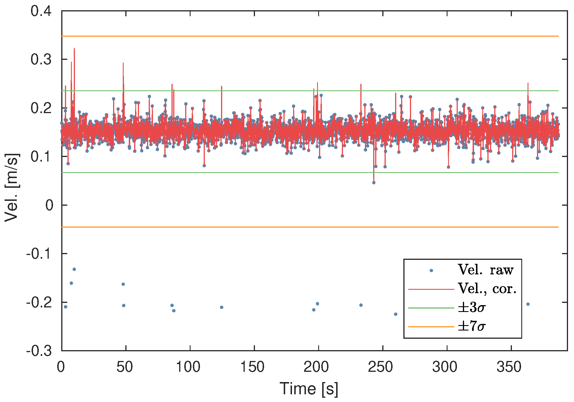
), but all ADV time series contained satisfactory beam correlations. The ambiguity velocity
was approximately 0.25 m/s for the ADCP, and ambiguity wrapping occurred in some situations in the longitudinally directed beams (
and
). Data points that exceeded
from the sample mean, where
is the sample standard deviation, were identified as artifacts due to ambiguity wrapping and were unwrapped
accordingly [
4].
Figure 3 shows an example of ambiguity-wrapped raw data (blue points) which are corrected (red line).
Some spikes occurred in the time series, resulting typically from unphysical data such as low correlation data, acoustic contamination specific to the laboratory or any of the other sources discussed in
Section 1, but also from natural extreme values. Following [
6], spikes were identified as data points that exceeded
from the sample mean (indicated in
Figure 3), which is similar to the minimum/maximum threshold filter described in [
16]. In calculations of statistical parameters, such as variance, the spikes were discarded. However, in spectral analysis, continuous time series are required, so it is necessary to replace the discarded data with artificial data to obtain a statistically equivalent dataset to the real dataset which would have been measured if there were no errors involved. Different approaches for replacement processes in the spectral analysis are reported in the literature. For example, ref. [
29] interpolate neighboring data points in case of low correlation which may lead to spikes, and [
6] include the spikes in the estimation of spectra. Both techniques will necessarily give some errors: due to the random nature of turbulence in the former case, especially if the turbulent scales are comparable to the sampling frequency, and the limited data quality in the latter case, particularly if there are solid boundaries in the vicinity of the instrument. In the present study, data points that exceeded
from the sample mean were simply “cut” to
from the sample mean, i.e. at the green lines in
Figure 3. This strategy may reduce the effect of natural extreme values but the noise from unphysical data is mitigated. Some spectra were estimated with both strategies, and they were almost identical, except that the spectra from the “cut” time series were marginally less energetic, which may indicate that the noise level was reduced.
Statistical analysis was performed on the quality-controlled data. Although homogeneity between the instantaneous beam velocities was not obtained for the ADCP, homogeneity was assumed in the mean and the variance of the signal [
1]. The mean longitudinal fluid velocity relative to the instrument
, where the angled brackets denote time averaging over the whole time series, was obtained directly from the longitudinal component of the ADV and from
of the ADCP [
1]. The fluctuating velocity component in any direction
was used in the turbulence analysis. Data that were flagged as spikes or with correlation less than the recommended values were discarded before calculating the velocity variance
. The component of the TKE in the transverse (vertical) direction
was defined as
. Since the transverse velocity was directly measured with the ADCP (
), no beam transformation was required to estimate
. Following [
9], the total TKE (denoted
in their paper)
was calculated as
for the ADV and the ADCP, respectively. Equation (
4) combines the variance estimates from the ADCP transducers according to vector algebra to estimate the Cartesian 3D variance components given in Equation (
3), with the assumption of homogeneity in variance over distances comparable to the horizontal separation of the bins [
9].
Turbulent kinetic energy frequency spectra
were estimated from the transverse (vertical) fluctuating velocity component
with the Welch method [
30], which means fast Fourier transformation and ensemble averaging of overlapping segments. Each time series was divided into segments of 1024 data points with 50% overlap and a Hamming window was applied to each segment to reduce spectral leakage. The TKE frequency spectra represent the distribution of turbulent kinetic energy over the frequencies
, where
is the Nyquist frequency, which was 4 and 100 Hz for the ADCP and the ADV, respectively. From
Figure 3, it is clear that
, which indicates that the advection of turbulence past the instrument is dominated by the mean flow and not by the circulation of eddies, and that the assumption of Taylor’s hypothesis is valid. Therefore, the TKE frequency spectra should be proportional to
in the inertial subrange.
Doppler noise often results in flat TKE frequency spectra, also known as the noise floor, towards the higher frequencies where the turbulent energy is low. From inspections of ADV data, it was observed that the noise floor was reached close to the Nyquist frequency, and the noise floor was found by averaging the 20 highest frequencies of the TKE spectra, which corresponds to frequencies in the range 96–100 Hz. Following [
31], the noise variance
of the ADV was estimated by integrating the noise floor over the range of frequencies
, assuming white noise spectra. The Doppler noise was removed from the ADV velocity variance statistically [
32] by subtracting the noise variance, so that
. It was not clear whether the ADCP spectra, which are shown in
Section 4, were obscured by noise. Hence, the turbulence properties obtained from the ADCP were not corrected for Doppler noise. Doppler noise is predominantly introduced in the horizontal velocity components in the case of ADVs, i.e., those ones perpendicular to the instrument axis [
15,
16]. Therefore, we mainly consider the velocity variance and spectra from the transverse (vertical) velocity component in this study.
4. Results and Discussion
The ADCP was able to reproduce the mean velocity in the longitudinal direction, as can be seen in
Figure 4a. For the cells located at the same vertical level as the ADV measurement volume, the errors were less than 4%. Some missing cells were discarded because the beam correlation criterion stated in
Section 3 (beam correlation must be greater than 50% more than 90% of the time) was not fulfilled. The measured velocities were about 10% lower than the towing speeds due to the grid-induced velocity deficit. The component of the TKE in the transverse direction
, non-dimensionalized over the square of the towing speed
, is presented in
Figure 4b. There was good agreement between the instruments for the high towing speed and the large grid, but the ADCP largely overestimated
in the other situations (by a factor of 2 for
U = 0.4 m/s and approximately 5 for
U = 0.2 m/s). A possible reason for this could be Doppler noise in the ADCP, which can cause a high bias in estimators related to TKE [
1]. As stated in
Section 3, estimated variance from the ADCP was not corrected for Doppler noise in the post processing.
Figure 4 indicates reasonable homogeneity of the flow in the transverse (vertical) direction. Similar experiments with ADV measurements in the same tank with identical grids, reported homogeneous turbulence levels in the lateral direction within ±0.5%, with the exception of a local increase of ±2% behind the frame holding the grid [
33].
Although the ADCP overestimated
in the transverse (vertical) direction, this was not the case for the total turbulent kinetic energy
estimated from Equations (
3) and (
4), presented in
Figure 5. For the high towing speed, the values estimated from the ADCP were up to 35% smaller than the equivalent ADV values. The instruments agreed fairly well for the low towing speed, although these estimates were quite scattered in the vertical profile. Doppler noise, which could vary between beams and cells, may have caused the deviations. Velocity components in all directions were used to estimate
. It was observed from the ADV data that the grid-generated turbulence was not very isotropic. The ratio of
was about 0.6, which is similar to the values obtained in another towing tank [
26]. In comparison, grid-generated turbulence in a wind tunnel could reach a ratio closer to unity, for example, ref. [
19] reported the ratio 0.8. Complete isotropy is not attainable in grid-generated turbulence due to the spatial inhomogeneity that arise from decay of TKE in the downstream direction [
19].
Figure 6 shows
versus downstream distance
for the large grid. The squares and triangles indicate the mean values obtained by ensemble averaging the ADCP cells located close to the ADV measurement volume in terms of depth. Typically, 11 cells were used to estimate the mean value, provided that all the time series satisfied the beam correlation criterion. A decay in
can be observed, and the transverse components of the TKE decrease with increasing downstream distance approximately as
, especially in the case of the ADV, which agrees with the findings of [
22,
26]. The ADCP data from the high towing speed approximately follow the same slope in the log-log plot, while the low towing speed data exhibit a weaker decay, which is in accordance with the mismatch observed between the ADV and the ADCP in
for the low towing speeds in
Figure 4b. The low towing speed data also have large error bars for increasing downstream distance. The error bars represent the spread of the data obtained from the different cells and show two standard deviations of the sample of (11) cells. We do not attempt to justify the existence of a power law, as the data hardly span over one decade in distance, and only three data points are considered.
Turbulent kinetic energy spectra estimated from the transverse (vertical) fluctuating velocity components of the two instruments are presented in
Figure 7. Spectra from the ADCP at 10 positions evenly distributed over the vertical profile are included, provided that the time series satisfied the beam correlation quality criterion. In general, it can be observed that the TKE level was higher with increasing towing speed and grid mesh size. The ADV spectra were proportional to the theoretical −5/3 power law over a wide range of frequencies, meaning that the instrument resolved the inertial subrange of turbulence. The ADV noise floor was reached well above 10 Hz and the noise level was approximately
. However, the ADCP was not able to resolve the inertial subrange. The ADCP spectra appear to be quite flat around
, which is consistent with the noise level of the Nortek Signature reported by [
3] from tidal channel measurements.
There are several possible explanations for the ADCP’s failing ability to resolve the inertial subrange of turbulence. First, Doppler noise seems to prevent the instrument from detecting turbulent energy below approximately
. This can be seen when the TKE starts to decrease with increasing frequency in accordance with the ADV spectra around 0.5 Hz, but then remain approximately constant. In other words, the TKE level at the scales associated with the inertial subrange in the flow may be too low to be detected by the instrument. On the other hand, it is not clear that the spectra flatten out in all situations. For example, in
Figure 7d), the ADCP spectra decay with increasing frequencies until the Nyquist frequency of 4 Hz is reached, although with a smaller rate than the slope of the ADV spectrum, which makes it difficult to conclude that the noise floor obscures the spectra.
Another possible explanation for the relatively flat spectra is the fact that the ADCP measurement volume is probably not adequately small to resolve the scales
associated with the inertial subrange. In fact, water flume experiments on grid-generated turbulence suggest that the integral scale of turbulence in the longitudinal direction
is approximately
at the downstream position
and slowly increasing with
[
27]. The same findings are reported in the wind tunnel experiments of [
21], who also found that the integral length scales
and
in the lateral and transverse directions, respectively, were about half the size of
. Assuming that the integral scale in the current experiments
L was approximately equal to
, it is possible to make order of magnitude estimates of the TKE dissipation rate
and the Reynolds numbers and eddy sizes at the various turbulent scales. Following [
34], the TKE dissipation rate is estimated from the ADV data as
, where
is a constant. The turbulence Reynolds number
, which is the Reynolds number of the eddies within the integral scales, can be expressed as
. In the inertial subrange, the eddies are associated with the Taylor microscale
and the Taylor microscale Reynolds number
, which can be estimated as
and
, respectively. In the dissipation range, the eddy size is associated with the Kolmogorov microcale
, which is determined by
and
through the relation
[
28].
The estimated TKE dissipation rates, Reynolds numbers and length scales summarized in
Table 2, indicate that the turbulent eddies were on the order of 10 cm, 1 cm and 1 mm in the integral, inertial and dissipation range, respectively, for all reported combinations of grid size and towing speed. The ADCP cell size was 2.5 and 5 cm for
U = 0.2 m/s and 0.4 m/s, respectively, which means that probably only the turbulent eddies in the integral scale were resolved by the instrument. However, the ADV measurement volume was approximately
, which suggests that the instrument was able to resolve turbulent eddies in the inertial subrange, according to
Table 2. This is also confirmed in
Figure 7, where the ADV spectra are proportional to the theoretical −5/3 slope over a wide range of frequencies. The Taylor microscale Reynolds numbers lie in the range of 120–290, which are typical values for fully developed grid-induced turbulence [
24,
25]. The turbulence Reynolds numbers are one order of magnitude smaller than the mesh Reynolds numbers.


