

Numerical Simulation of Taylor—Couette—Poiseuille Flow at Re = 10,000

Abstract
:1. Introduction
2. Problem Statement and Numerical Algorithm
3. Results and Discussion
3.1. Mean Flow Properties and Turbulence Statistics
- Case 1: and .
- Case 2: and .
- Case 3: and .
3.2. Flow Patterns, Vortical and Turbulence Structures
3.3. Integral Parameters
4. Conclusions
- Rotation leads to a thinning of the viscous sublayer and, as a consequence, a widening of the mean axial profile and an increase in gradients at the wall. The axial velocity component distribution in wall units decreases due to an increase in friction on the wall with increasing rotation N.
- Rotation decreases axial fluctuation production and increases tangential fluctuation production in wall units, while the maximum value of total production is weakly dependent on rotation, but its position shifts towards the wall into the buffer zone.
- With increase in rotation and , the following changes are observed:
- –
- The tangential velocity component changes its shape, eliminating the local maximum at about one-third of the channel width from the inner wall.
- –
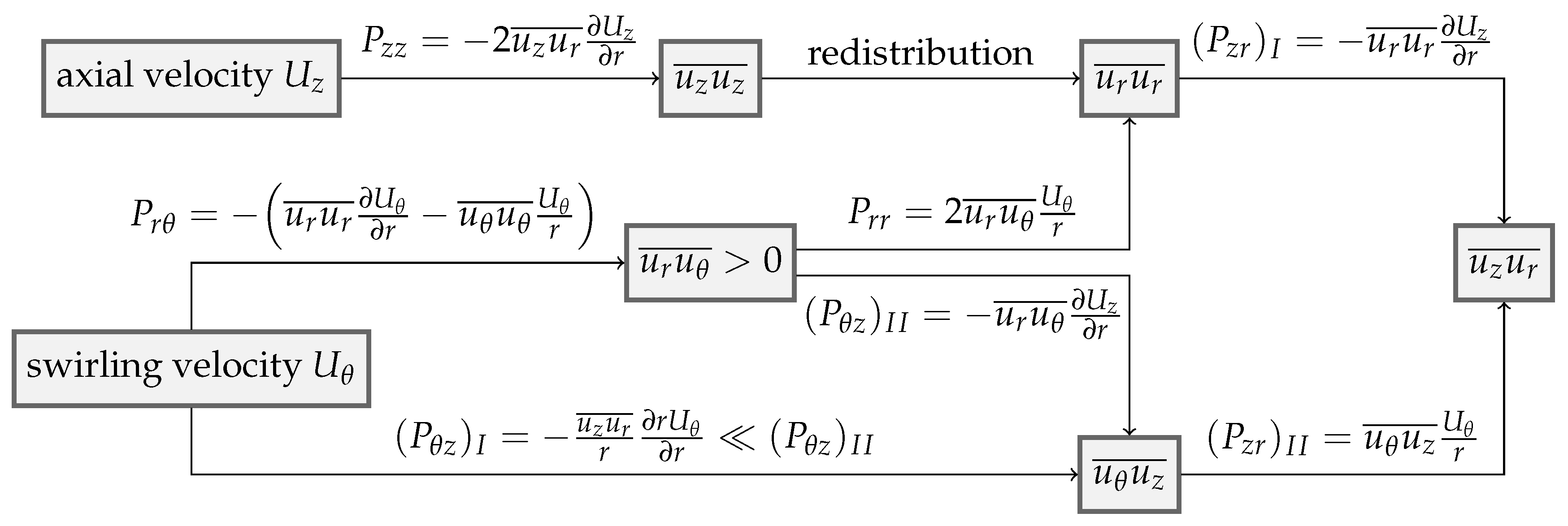
- The profile of the Reynolds stress tensor component changes its monotonicity and becomes positive in areas where it was not before.
- –
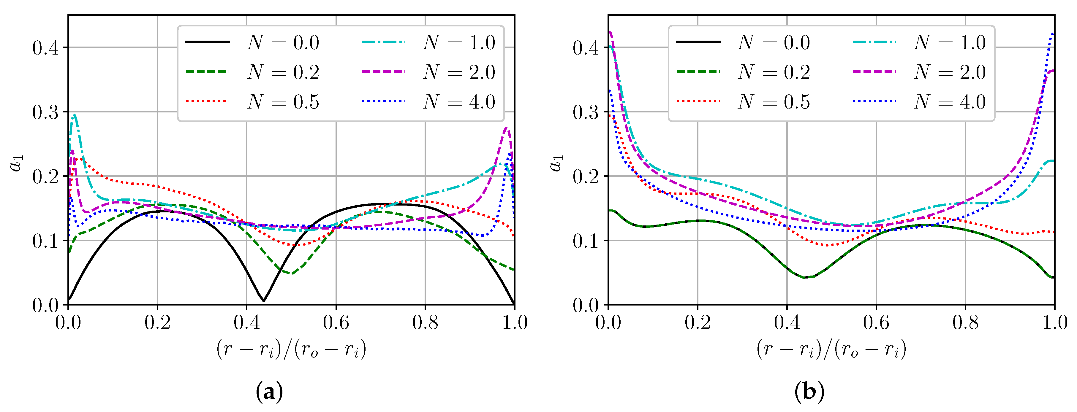
- The structural parameter begins to decrease with increasing rotation, i.e., the production of shear components becomes less efficient.
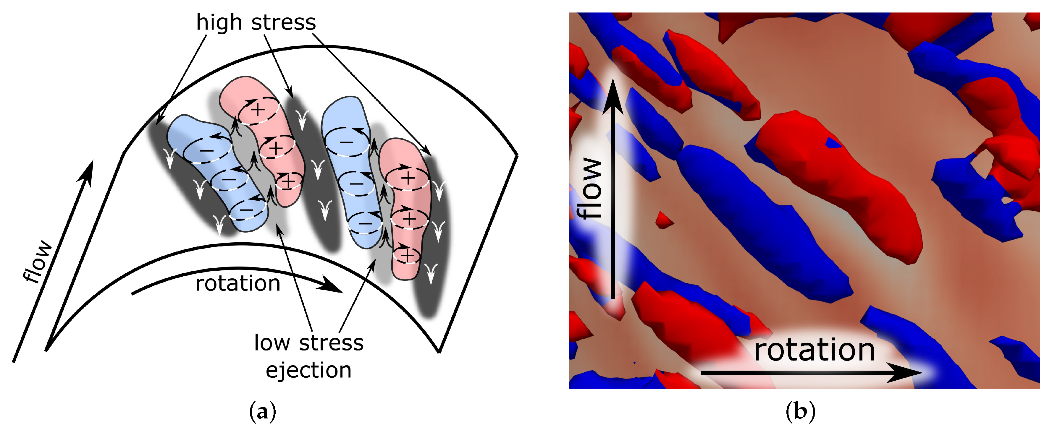
- The applicability of URANS and EBM techniques for describing first and second statistical moments of velocity fluctuation as well as integral characteristics of the flow is shown. URANS describes the vortex structures of the flow well, however, in an enlarged form.
Author Contributions
Funding
Data Availability Statement
Acknowledgments
Conflicts of Interest
Nomenclature
| structure parameter = | |
| skin friction factor = | |
| hydraulic diameter = | |
| k | turbulent kinetic energy = |
| computational length in the z direction | |
| N | rotation rate = |
| number of mesh points in the directions, respectively | |
| production of Reynolds stress tensor | |
| radius of inner and outer cylinder, respectively | |
| Re | Reynolds number based on characteristic velocity and length scales |
| symmetric component of the velocity gradient tensor | |
| mean velocity components in the directions, respectively | |
| bulk axial velocity | |
| inner cylinder rotation velocity | |
| friction velocity = | |
| fluctuating velocity components in the directions, respectively | |
| T | dimensionless torque = |
| y | distance from the inner or outer wall |
| mesh spacing in the directions, respectively | |
| second largest eigenvalue of | |
| anti-symmetric component of the velocity gradient tensor | |
| density of fluid | |
| statistically averaged wall shear stress in the directions, respectively at the inner or outer wall | |
| value in wall units, normalized by , | |
| value related to inner or outer wall, respectively | |
| root mean square value | |
| Abbreviations | |
| CFL | Courant–Friedrichs–Lewy number |
| DNS | Direct Numerical Simulation |
| LES | Large Eddy Simulation |
| URANS | Unstationary Reynolds Average Navier–Stokes |
| RANS | Reynolds Average Navier–Stokes |
| RSM | Reynolds Stress Model |
| r.m.s. | root mean square |
| EBM | Elliptic Blending Model |
| QUICK | Quadratic Upstream Interpolation for Convective Kinematics |
| TKE | Turbulence Kinetic Energy (k) |
Appendix A


| Discretization Parameters | T | ||||||
|---|---|---|---|---|---|---|---|
| Value | , % |
GCI, %, | | Value | , % |
GCI, %, | | ||
| 1 | 1 | 0.0120902 | 2.0 | 3.6|1.3 | 10.12200 | − 8.6 | 3.5|6.2 |
| 1 | 0.666 | 0.0121562 | 2.6 | −|− | 10.39252 | −6.1 | −|− |
| 1 | 1.5 | 0.0114605 | −3.3 | −|4.2 | 9.68278 | −12.5 | −|5.0 |
| 0.666 | 1 | 0.0119124 | 0.5 | −|− | 9.97591 | −9.9 | −|− |
| 0.83 | 1 | 0.0119603 | 0.9 | 2.2|− | 10.02131 | −9.5 | 2.5|− |
| 0 | 0 | 0.0118497 | 0 | − | 11.06893 | 0 | − |
| Discretization Parameters | T | ||||||
|---|---|---|---|---|---|---|---|
| Value | , % |
GCI, %, | | Value | , % |
GCI, %, | | ||
| 1 | 1 | 0.011135 | −8.3 | 1.0|6.8 | 9.25550 | −17.0 | 0.9|11.5 |
| 1 | 0.666 | 0.011460 | −5.6 | −|− | 9.72499 | −12.8 | −|− |
| 1 | 0.8 | 0.011317 | −6.8 | −|8.5 | 9.40816 | −15.6 | −|22.1 |
| 0.5 | 1 | 0.011028 | −9.1 | −|− | 9.17314 | −17.7 | −|− |
| 0.75 | 1 | 0.011092 | −8.6 | 1.4|− | 9.20806 | −17.4 | 0.9|− |
| 0 | 0 | 0.012137 | 0 | − | 11.15210 | 0 | − |
References
- Hadžiabdić, M.; Hanjalić, K.; Mullyadzhanov, R. LES of turbulent flow in a concentric annulus with rotating outer wall. Int. J. Heat Fluid Flow 2013, 43, 74–84. [Google Scholar] [CrossRef]
- Nouri, J.M.; Umur, H.; Whitelaw, J.H. Flow of Newtonian and non-Newtonian fluids in concentric and eccentric annuli. J. Fluid Mech. 1993, 253, 617. [Google Scholar] [CrossRef]
- Nouri, J.M.; Whitelaw, J.H. Flow of Newtonian and Non-Newtonian Fluids in a Concentric Annulus With Rotation of the Inner Cylinder. J. Fluids Eng. 1994, 116, 821–827. [Google Scholar] [CrossRef]
- Nouri, J.; Whitelaw, J. Flow of Newtonian and non-Newtonian fluids in an eccentric annulus with rotation of the inner cylinder. Int. J. Heat Fluid Flow 1997, 18, 236–246. [Google Scholar] [CrossRef]
- Escudier, M.P.; Gouldson, I.W.; Jones, D.M. Flow of shear-thinning fluids in a concentric annulus. Exp. Fluids 1995, 18, 225–238. [Google Scholar] [CrossRef]
- Rothe, T.; Pfitzer, H. The influence of rotation on turbulent flow and heat transfer in an annulus between independently rotating tubes. Heat Mass Transf. 1997, 32, 353–364. [Google Scholar] [CrossRef]
- Chung, S.Y.; Rhee, G.H.; Sung, H.J. Direct numerical simulation of turbulent concentric annular pipe flow. Int. J. Heat Fluid Flow 2002, 23, 426–440. [Google Scholar] [CrossRef]
- Jung, S.Y.; Sung, H.J. Characterization of the three-dimensional turbulent boundary layer in a concentric annulus with a rotating inner cylinder. Phys. Fluids 2006, 18, 115102. [Google Scholar] [CrossRef]
- Chung, S.Y.; Sung, H.J. Large-eddy simulation of turbulent flow in a concentric annulus with rotation of an inner cylinder. Int. J. Heat Fluid Flow 2005, 26, 191–203. [Google Scholar] [CrossRef]
- Poncet, S.; Viazzo, S.; Oguic, R. Large eddy simulations of Taylor-Couette-Poiseuille flows in a narrow-gap system. Phys. Fluids 2014, 26, 105108. [Google Scholar] [CrossRef]
- Piton, M.; Huchet, F.; Cazacliu, B.; Corre, O.L. Numerical Turbulent Flow Analysis through a Rotational Heat Recovery System. Energies 2022, 15, 6792. [Google Scholar] [CrossRef]
- Ohsawa, A.; Murata, A.; Iwamoto, K. Through-flow effects on Nusselt number and torque coefficient in Taylor-Couette-Poiseuille flow investigated by large eddy simulation. J. Therm. Sci. Technol. 2016, 11, JTST0031. [Google Scholar] [CrossRef]
- Hanjalic, K.; Launder, B. Modelling Turbulence in Engineering and the Environment; Cambridge University Press: Cambridge, UK, 2011. [Google Scholar] [CrossRef]
- Poncet, S.; Haddadi, S.; Viazzo, S. Numerical modeling of fluid flow and heat transfer in a narrow Taylor–Couette–Poiseuille system. Int. J. Heat Fluid Flow 2011, 32, 128–144. [Google Scholar] [CrossRef]
- Pawar, S.B.; Thorat, B. CFD simulation of Taylor–Couette flow in scraped surface heat exchanger. Chem. Eng. Res. Des. 2012, 90, 313–322. [Google Scholar] [CrossRef]
- Gavrilov, A.; Ignatenko, Y.; Bocharov, O.; Aragall, R. Turbulent Flow Simulation of Power-Law Fluid in Annular Channel. In Proceedings of the ASME 2020 39th International Conference on Ocean, Offshore and Arctic Engineering, Virtual, 3–7 August 2020. [Google Scholar] [CrossRef]
- Naser, A. Prediction of Newtonian and non-Newtonian flow through concentric annulus with centerbody rotation. In Proceedings of the 1st International Conference on CFD in Mineral and Metal Processing and Power Generation, Melbourne, Australia, 3–4 July 1997. [Google Scholar]
- Elena, L.; Schiestel, R. Turbulence modeling of rotating confined flows. Int. J. Heat Fluid Flow 1996, 17, 283–289. [Google Scholar] [CrossRef]
- Reynolds, W.C. Towards A Structure-Based Turbulence Model. In Studies in Turbulence; Springer: New York, NY, USA, 1992; pp. 76–80. [Google Scholar] [CrossRef]
- Reynolds, W.C.; Kassinos, S.C. One-Point Modelling of Rapidly Deformed Homogeneous Turbulence. Proc. Math. Phys. Sci. 1995, 451, 87–104. [Google Scholar]
- Cambon, C.; Jacquin, L.; Lubrano, J.L. Toward a new Reynolds stress model for rotating turbulent flows. Phys. Fluids Fluid Dyn. 1992, 4, 812–824. [Google Scholar] [CrossRef]
- Lockett, T.J. Numerical Simulation of Inelastic Non-Newtonian Fluid Flows in Annuli. Ph.D. Thesis, Imperial College of Science Technology and Medicine, University of London, London, UK, 1992. [Google Scholar]
- Piton, M.; Huchet, F.; Cazacliu, B.; Corre, O.L. Heat Transport in Rotating Annular Duct: A Short Review. Energies 2022, 15, 8633. [Google Scholar] [CrossRef]
- Manceau, R. Recent progress in the development of the Elliptic Blending Reynolds-stress model. Int. J. Heat Fluid Flow 2015, 51, 195–220. [Google Scholar] [CrossRef]
- Gavrilov, A.A.; Rudyak, V.Y. Direct numerical simulation of the turbulent energy balance and the shear stresses in power-law fluid flows in pipes. Fluid Dyn. 2017, 52, 363–374. [Google Scholar] [CrossRef]
- Germano, M.; Piomelli, U.; Moin, P.; Cabot, W.H. A dynamic subgrid-scale eddy viscosity model. Phys. Fluids Fluid Dyn. 1991, 3, 1760–1765. [Google Scholar] [CrossRef]
- Lilly, D.K. A proposed modification of the Germano subgrid-scale closure method. Phys. Fluids Fluid Dyn. 1992, 4, 633–635. [Google Scholar] [CrossRef]
- Sagaut, P. Large Eddy Simulation for Incompressible Flows; Springer: Berlin/Heidelberg, Germany, 2006. [Google Scholar] [CrossRef]
- Pope, S.B. Turbulent Flows; Cambridge University Press: Cambridge, UK, 2000. [Google Scholar] [CrossRef]
- Hirai, S.; Takagi, T. Parameters dominating swirl effects on turbulent transport derived from stress-scalar-flux transport equation. Int. J. Heat Mass Transf. 1995, 38, 2175–2182. [Google Scholar] [CrossRef]
- Floryan, J.M. Görtler instability of boundary layers over concave and convex walls. Phys. Fluids 1986, 29, 2380. [Google Scholar] [CrossRef]
- Dong, S. Direct numerical simulation of turbulent Taylor–Couette flow. J. Fluid Mech. 2007, 587, 373–393. [Google Scholar] [CrossRef]
- Ignatenko, Y.S.; Gavrilov, A.A.; Bocharov, O.B. On Spiral Turbulent Flow in an Annular Concentric Channel. J. Phys. Conf. Ser. 2021, 1867, 012010. [Google Scholar] [CrossRef]
- Hanjalić, K.; Launder, B.E. Eddy-Viscosity Transport Modelling: A Historical Review. In 50 Years of CFD in Engineering Sciences; Springer: Singapore, 2020; pp. 295–316. [Google Scholar] [CrossRef]
- Hanjalić, K.; Launder, B.E. Reassessment of modeling turbulence via Reynolds averaging: A review of second-moment transport strategy. Phys. Fluids 2021, 33, 091302. [Google Scholar] [CrossRef]
- Oberkampf, W.L.; Roy, C.J. Verification and Validation in Scientific Computing; Cambridge University Press: Cambridge, UK, 2010. [Google Scholar] [CrossRef]


| N | 0 | 0.2 | 0.5 | 1 | 2 | 4 |
|---|---|---|---|---|---|---|
| 0.85 ± 0.14 | 0.79 ± 0.14 | 0.79 ± 0.16 | 0.98 ± 0.21 | 0.93 ± 0.2 | 0.55 ± 0.25 | |
| 0.74 ± 0.13 | 0.67 ± 0.12 | 0.47 ± 0.08 | 0.71 ± 0.13 | 0.78 ± 0.15 | 0.75 ± 0.12 | |
| 8.22 ± 1.37 | 7.63 ± 1.35 | 9.56 ± 1.91 | 13.03 ± 2.83 | 9.36 ± 2.05 | 14.47 ± 3.19 | |
| 7.68 ± 1.31 | 6.97 ± 1.22 | 7.79 ± 1.37 | 9.44 ± 1.75 | 5.9 ± 1.14 | 16.11 ± 2.25 | |
| 4.49 ± 0.75 | 4.18 ± 0.74 | 5.31 ± 1.06 | 11.41 ± 2.48 | 10.24 ± 2.24 | 20.24 ± 4.46 | |
| 8.37 ± 1.43 | 7.61 ± 1.33 | 8.65 ± 1.52 | 16.51 ± 3.05 | 12.89 ± 2.49 | 11.28 ± 2.25 | |
| CFL | 0.67 ± 0.28 | 0.75 ± 0.29 | 0.73 ± 0.25 | 0.7 ± 0.21 | 0.73 ± 0.23 | 0.88 ± 0.27 |
| N | 0.2 | 0.5 | 1 | 2 | 4 |
|---|---|---|---|---|---|
| 0.8 ± 0 | 0.82 ± 0.14 | 0.94 ± 0.2 | 0.9 ± 0.22 | 0.74 ± 0.16 | |
| 1.42 ± 0 | 1.2 ± 0.02 | 1.2 ± 0.12 | 1.0 ± 0.1 | 0.8 ± 0.06 | |
| 25.61 ± 0 | 29.32 ± 4.97 | 29.39 ± 6.53 | 27.58 ± 6.53 | 28.55 ± 6.41 | |
| 24.06 ± 0 | 24.09 ± 0.5 | 21.32 ± 1.93 | 16.97 ± 1.63 | 15.69 ± 1.35 | |
| 16.64 ± 0 | 17.94 ± 3.04 | 20.11 ± 4.47 | 23.24 ± 5.5 | 26.7 ± 6 | |
| 31.22 ± 0 | 29.43 ± 0.61 | 29.13 ± 2.63 | 28.57 ± 2.74 | 29.32 ± 2.52 | |
| CFL | 0.44 ± 0.17 | 0.46 ± 0.16 | 0.60 ± 0.18 | 0.77 ± 0.29 | 0.63 ± 0.19 |
| N | LES | URANS | EBM | k- SST | |
|---|---|---|---|---|---|
| 0 | 0.00864 | 0.00921 (+6.6%) | 0.00903 (+4.5%) | 0.00921 (+6.6%) | |
| 0.2 | 0.00946 | 0.00925 (−2.2%) | 0.00903 (−4.6%) | 0.00925 (−2.2%) | |
| 0.5 | 0.01214 | 0.01192 (−1.8%) | 0.01074 (−12%) | 0.00969 (−20%) | |
| 1 | 0.01659 | 0.01537 (−7.4%) | 0.01423 (−14%) | 0.01065 (−36%) | |
| 2 | 0.02311 | 0.02122 (−8.2%) | 0.02138 (−7.5%) | 0.01364 (−41%) | |
| 4 | 0.03493 | 0.02940 (−16%) | 0.03385 (−3.1%) | 0.01712 (−51%) | |
| 0 | 0.00754 | 0.00819 (+8.6%) | 0.00810 (+7.2%) | 0.00819 (+8.6%) | |
| 0.2 | 0.00778 | 0.00823 (+5.8%) | 0.00810 (+4.1%) | 0.00823 (+5.8%) | |
| 0.5 | 0.00853 | 0.00820 (−3.9%) | 0.00834 (−2.2%) | 0.00842 (−1.2%) | |
| 1 | 0.00984 | 0.00899 (−8.7%) | 0.00935 (−4.9%) | 0.00866 (−12%) | |
| 2 | 0.01294 | 0.01129 (−13%) | 0.01256 (−2.9%) | 0.00992 (−23%) | |
| 4 | 0.01979 | 0.01521 (−23%) | 0.01989 (0.5%) | 0.01169 (−41%) |
Disclaimer/Publisher’s Note: The statements, opinions and data contained in all publications are solely those of the individual author(s) and contributor(s) and not of MDPI and/or the editor(s). MDPI and/or the editor(s) disclaim responsibility for any injury to people or property resulting from any ideas, methods, instructions or products referred to in the content. |
© 2023 by the authors. Licensee MDPI, Basel, Switzerland. This article is an open access article distributed under the terms and conditions of the Creative Commons Attribution (CC BY) license (https://creativecommons.org/licenses/by/4.0/).
Share and Cite
Gavrilov, A.; Ignatenko, Y. Numerical Simulation of Taylor—Couette—Poiseuille Flow at Re = 10,000. Fluids 2023, 8, 280. https://doi.org/10.3390/fluids8100280
Gavrilov A, Ignatenko Y. Numerical Simulation of Taylor—Couette—Poiseuille Flow at Re = 10,000. Fluids. 2023; 8(10):280. https://doi.org/10.3390/fluids8100280
Chicago/Turabian StyleGavrilov, Andrey, and Yaroslav Ignatenko. 2023. "Numerical Simulation of Taylor—Couette—Poiseuille Flow at Re = 10,000" Fluids 8, no. 10: 280. https://doi.org/10.3390/fluids8100280